Single-cell RNA-seq clustering: datasets, models, and algorithms

ABSTRACT

Single-cell RNA sequencing (scRNA-seq) technologies allow numerous opportunities for revealing novel and potentially unexpected biological discoveries. scRNA-seq clustering helps elucidate cell-to-cell heterogeneity and uncover cell subgroups and cell dynamics at the group level. Two important aspects of scRNA-seq data analysis were introduced and discussed in the present review: relevant datasets and analytical tools. In particular, we reviewed popular scRNA-seq datasets and discussed scRNA-seq clustering models including K-means clustering, hierarchical clustering, consensus clustering, and so on. Seven state-of-the-art scRNA clustering methods were compared on five public available datasets. Two primary evaluation metrics, the Adjusted Rand Index (ARI) and the Normalized Mutual Information (NMI), were used to evaluate these methods. Although unsupervised models can effectively cluster scRNA-seq data, these methods also have challenges. Some suggestions were provided for future research directions.

KEYWORDS:

• ScRNA-seq
• cell clustering
• K-means clustering
• hierarchical clustering
• consensus clustering

1. Introduction

Identifying cell lineages within tissues or organisms is one of the most important goals of modern biological sciences. Evaluating these associations will greatly increase our understanding of tissue development and homoeostasis [1,2]. Moreover, a complete understanding of these relationships will allow the identification of developmental disorders and pathologies, in addition to providing targets to mitigate disease states including cancer [3–5]. Lineage families have traditionally been detected by introducing a heritable label into a cell and following its progeny.

Recently, lineage tracing has been conducted by identifying cell types using single-cell transcriptomics [6,7,]. Different cell types comprising the progeny are developmentally associated because their labelled genes all originated from an identical founder cell. Furthermore, the diversity of cell types within the offspring population represents the potential of the founder cell [1,8,]. To precisely infer the potential, lineage tracing requires effective identification of cell-types. Ideally, several markers would be used to conduct accurate cell-type classifications. However, marker numbers are limited, which could possibly mask the variability observed within a group of cells that express the screened marker genes. Consequently, lineage tracing can result in biases [9,10,].

Single-cell RNA sequencing (scRNA-seq) technologies have increasingly allowed the probing of cell types over the past decade. scRNA-seq can help identify complex and rare cell type groups, help identify gene regulatory associations, aid the evaluation of developmental trajectories of different cell lineages, and help reveal cell-to-cell variabilities within various diseases and therapeutic contexts [1,11–17]. The initial analysis of scRNA-seq data mainly involves clustering and annotation of individual cells into cell types based on their transcriptomes. Such analyses can inform our understanding of the biological characteristics that distinguish different cell groups, tumour cell heterogeneities, and cellular diversities from local tumour microenvironments. More importantly, while bulk tumour transcriptomes can help reveal therapeutic sensitivity, scRNA-seq can improve the inference of treatment efficacy by allowing identification of transcriptomic differences in coexisting tumour groups [18–21].

Many clustering algorithms have recently been developed to identify cell type-like structures from scRNA-seq datasets. These methods are generally developed on the assumption that cells of a particular type have similar transcriptomes that differ from other cell types in tissues [22–27]. In this study, we evaluated the use of scRNA-seq data in the development of analysis tools that are primarily associated with scRNA-seq clustering techniques including K-means clustering, hierarchical clustering, and consensus clustering. Moreover, we evaluated metrics for measuring clustering performances while comparing the clustering models and providing suggestions for future research directions.

2. Materials and methods

2.1. ScRNA-seq datasets

Published studies were gathered, and we summarized 20 scRNA-seq datasets from these including the provider, number of cells, number of genes, and cell resources (Table 1).

Table 1. ScRNA-seq datasets.

Dataset	Num. of cells	Num. of genes	Cell resource
Trapnell [28]	182	38,694	Myogenic precursor cells and differentiating myoblast cells	https://www.ebi.ac.uk/biostudies/studies/S-EPMC4122333?xr=true
Petropoulos [29]	1,529	3,000	Human preimplantation embryonic cells	ArrayExpress (https://www.ebi.ac.uk/arrayexpress/)
Biase [72]	49	25,737	2-cell and 4-cell mouse embryos	GEO (https://www.ncbi.xilesou.top/)
Yan’s [30]	124	22,687	Human preimplantation embryos and embryonic stem cells	GEO (https://www.ncbi.xilesou.top/)
Goolam [31]	124	41,480	4-cell mouse embryos	GEO (https://www.ncbi.xilesou.top/)
Pollen [70]	301	23,730	Human cerebral cortex	GEO (https://www.ncbi.xilesou.top/)
Kolodziejczyk’s [32]	704	38,653	Mouse embryonic stem cell	ArrayExpress (https://www.ebi.ac.uk/arrayexpress/)
Treutlein [33]	80	23,271	Distal lung epithelium	GEO (https://www.ncbi.xilesou.top/)
Ting [34]	149	29,018	Pancreatic circulating tumour cells	GEO (https://www.ncbi.xilesou.top/)
Patel [35]	430	5,948	Glioblastoma	PubMed (https://www.ncbi.xilesou.top/)
Usoskin [36]	622	25,334	Sensory neuron	GEO (https://www.ncbi.xilesou.top/)
Klein [37]	2,717	24,175	Embryonic stem cells	GEO (https://www.ncbi.xilesou.top/)
Zeisel [38]	3,005	19,972	Mouse cortex and hippocampus	GEO (https://www.ncbi.xilesou.top/)
Deng [39]	268	22,457	Mammalian cells	Science (https://www.sciencemag.org/)
Peng [81]	14,032	93,951	Peripheral blood mononuclear cells in systemic lupus erythematosus patients	https://github.com/ChengF-Lab/COAC
MacParland [40]	8,444	20,007	Parenchymal and non-parenchymal cells from five human livers	https://github.com/BaderLab/singleLiverCells
Yang [58]	500	32,738	Peripheral blood mononuclear cells	http://support.10xgenomics.com/single-cell/datasets
Shekhar [41] Darmanis [69] Xu [71]	27,499 420 540	13,166 22,085 56,650	Mouse retinal bipolar cells Human brain Idiopathic pulmonary fibrosis	GEO (https://www.ncbi.xilesou.top/) GEO (https://www.ncbi.xilesou.top/) GEO (https://www.ncbi.xilesou.top/)

2.2. Data analysis tools

Several analytical tools have recently been developed to facilitate the visualization of scRNA-seq data and identify subpopulations of cells. Twelve popular scRNA-seq analysis tools are summarized below.

2.2.1. DendroSplit

Zhang et al. [42] developed a clustering framework, DendroSplit [42] (https://github.com/jessemzhang/dendrosplit), for clustering cellular data. The tool emphasizes interpretability and is comparable in speed and accuracy to existing cluster models.

2.2.2. SinCHet

Li et al. [43] developed an analytical framework for continuous data (e.g., mRNA expression data) and binary omics data (e.g., discretized methylation) via a graphical user interface, SinCHet [43] (http://labpages2.moffitt.org/chen/software/). The toolkit can quantify cellular heterogeneity at different clonal resolutions. In particular, it aids in the identification of emerging or disappearing clones and prioritizing biomarkers based on markers or variation between (or within) cellular populations.

2.2.3. Scater

McCarthy et al. [44] developed a bioconductor package, Scater [44] (http://bioconductor.org/packages/scater), to pre-process, normalize, and visualize scRNA-seq data. The package provides a convenient and flexible pipeline to transform raw sequencing reads into a reliable expression dataset that can be applied to downstream analyses.

2.2.4. SPRING

Weinreb et al. [45] developed a more reproducible stochastic visualization workflow, SPRING [45] (https://kleintools.hms.harvard.edu/tools/spring.html), that can filter, normalize, and visualize scRNA-seq data. SPRING has been used to uncover detailed biological associations by visualizing gene expression trajectories from upper airway epithelial cells and haematopoietic progenitor cells.

2.2.5. ASAP

Gardeux et al. [46] designed a fully integrated platform, ASAP [46] (https://github.com/DeplanckeLab/ASAP), to analyse scRNA-seq data. ASAP is web-based and combines various supervised learning methods with sophisticated visualization tools. The package can parse, filter, normalize, and visualize scRNA-seq data. In addition, it can help detect cellular subpopulations, differentially expressed genes, and functional gene enrichments. More importantly, it can be broadly applied to any RNA-seq dataset if there is an overlap between bulk RNA-seq and scRNA-seq analysis pipelines.

2.2.6. SIMLR

Wang et al. [47] described an open-source, large-scale genomic analysis tool, SIMLR [47] (https://github.com/BatzoglouLabSU/SIMLR), that learns sample-to-sample similarity from gene expression data of heterogeneous samples. SIMLR can effectively reduce the dimensionality of scRNA-seq data, cluster scRNA-seq data, and visualize heterogeneous populations. In addition, the package provides greater interpretability through useful visualizations.

2.2.7. SCANPY

Wolf et al. [48] designed a scalable tool, SCANPY [48] (https://github.com/theislab/Scanpy), to analyse single-cell gene expression data. SCANPY can preprocess, visualize, and cluster single-cell datasets for over one million cells. In addition, the package can perform tests of differential expression, pseudo-time and trajectory inference, and simulation of gene regulatory networks.

2.2.8. TSCAN

Ji Z. and Ji H. [49] developed the single-cell analysis tool, TSCAN [49] (https://zhiji.shinyapps.io/TSCAN/), to better reconstruct in silico pseudo-temporal paths in scRNA-seq analysis. TSCAN is web-based and can read and preprocess scRNA-seq data, rank cells according to transitions of their transcriptomes, and perform differential gene analysis and single gene visualization.

2.2.9. FastProject

DeTomaso D. and Yosef N. [50] developed the software package, FastProject [50] (https://github.com/YosefLab/FastProject/wiki), to analyse and interpret scRNA-seq data and explore two-dimensional projections of these data. FastProject can also systematically investigate biological associations between these low-dimensional representations by integrating domain knowledge.

2.2.10. Granatum

Zhu et al. [51] developed an easy-to-use graphical interface, Granatum [51] (http://garmiregroup.org/granatum/app), to analyse scRNA-seq data. Granatum is web-based and contains a comprehensive list of functions including batch-effect removal, outlier-sample removal, gene filtering, gene-expression normalization, imputation, cell clustering, differential gene expression/enrichment analysis, cellular pseudo-time pathway construction, and visualization of protein interaction networks.

2.2.11. FIt-SNE

Linderman et al. [52] combined t-distributed stochastic neighbour embedding (t-SNE) and designed an advanced version of t-SNE for scRNA-seq data analysis, FIt-SNE [52] (https://github.com/KlugerLab/FIt-SNE), to visualize rare cell populations. Importantly, they still implemented a heatmap-style visualization (https://github.com/KlugerLab/t-SNE-Heatmaps) of scRNA-seq data based on one-dimensional t-SNE in order to simultaneously visualize the expression patterns for thousands of genes.

2.2.12. SC3

Kiselev et al. [27] presented a user-friendly tool, SC3 [27] (http://bioconductor.org/packages/SC3), to quantify the characterization of cell types by combining global transcriptome profiles. In particular, SC3 can identify subclones from the transcriptomes of neoplastic cells.

2.3. Clustering methods

Given that gene expression data for $p$ genes on $n$ cells can be organized into a $p\times n$ matrix $x=(x_1,x_2,...,x_n)$, $x_i$ denotes the gene expression profile of $p$ genes in cell $i$ and $x_i=(x_{i1},x_{i2},...,x_{ip}{)}^{\prime }$. Various clustering models can then be used to identify cell subpopulations based on expression data.

2.3.1. K-means clustering

2.3.1.1. RaceID

Grün et al. [53] surmised that detecting rare cell types like cancer stem cells and circulating tumour cells is important for understanding the biological characteristics of normal and diseased tissues. They developed an identification method for rare cell types (RaceID) based on a K-means clustering algorithm. RaceID comprises the following two steps:

Step 1. Preprocessing

RaceID removes cells with low transcript levels, and then normalizes the total transcript counts of each cell, finally filters out genes with very low or high expressed values.

Step 2. Clustering

RaceID computes the similarity between two cells based on Pearson’s correlation coefficients. A distance matrix equivalent to 1 minus the coefficient is then used as the distance matrix input for a K-means clustering algorithm in order to identify rare cell types from the gap statistic.

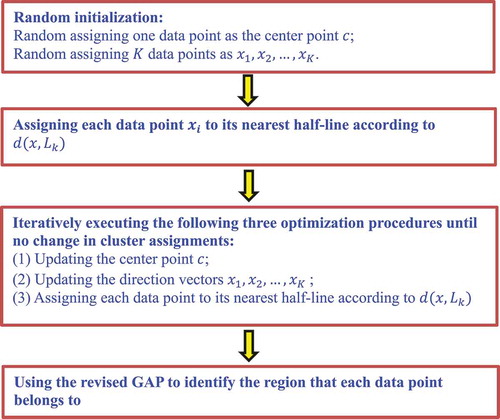
2.3.1.2. K-branches clustering

Chlis et al. [54] developed the K-Branches clustering algorithm. The algorithm introduced a clustering method similar to K-means and locally fitted half-lines to represent the branches of differentiation trajectory. It can identify the precise number of ‘tip regions’ or ‘branching regions’ in a lineage tree. The K-branches clustering method comprises two steps:

Step 1. Calculate the distance between half-line and data point and assign all data to the nearest half-line.

Step 2. Update centre $c$ and direction $v$ of a cluster until the total cost $j$ stops descending and obtain the final clusters.

The K-branches clustering method is similar to the K-means clustering method when computing distance. They are based on the Euclidean distance. However, for the K-means clustering algorithm, the distance computation severely affects the centre of a cluster. More importantly, the selection of the clustering centre is greatly influenced by noisy data that are far away from other samples. Therefore, the K-means clustering algorithm is not suitable to cluster non-spherical data. However, the K-branches clustering method iteratively selects data from a cluster to represent the centre $c$ of the cluster, and then computes the sum of the distances between the remaining data and the centre $c$ to split these data to the nearest half-line. The K-branches clustering algorithm developed a revised GAP statistic method to find whether a data point is at a branch tip, intermediate region or branching region of a lineage tree (Fig. 1).

Figure 1. Flowchart of the K-branches clustering method.

2.3.2. Hierarchical clustering

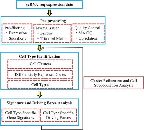
2.3.2.1. SINCERA

Guo et al. [55] presented a computational framework for SINgle Cell RNA-seq profiling Analysis (SINCERA) to distinguish and evaluate major cell types, infer gene signatures related to cell types, and determine key factors for cell type identification and activity (driving forces). SINCERA consists of three major analytical procedures: pre-processing of related data, identifying cell types, and analysing gene signatures and driving forces (Fig. 2).

Figure 2. Flowchart of single-cell RNA-seq profiling analysis.

2.3.2.2. BISCUIT

Prabhakaran et al. [56] considered that various single-cell gene expression data can be obtained by using emerging technologies. But these expression data are interfered by the error of technologies or cell description. Global normalization is a universal solution; however, it can not fundamentally solve the problem: it failed to resolve missing data and did not consider technical variation, thereby severely depending on latent cell types. Therefore, they developed a Bayesian Inference method for Single-cell ClUstering and ImpuTing (BISCUIT). BISCUIT integrates iterative normalization and a hierarchical Dirichlet process mixture model. It can be iteratively applied to dropout data and clustering. More importantly, it eliminates technical variation caused by different biological signals.

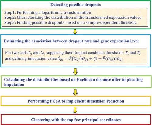
2.3.2.3. CIDR

Lin et al. [24] designed the ultrafast algorithm Clustering through Imputation and Dimensionality Reduction (CIDR) to decrease the impact of dropouts on clustering performance. The CIDR framework comprises five steps:

Step 1. Detect possible dropouts.

CIDR first performs a logarithmic transformation of gene expression data for each cell $C_i$. It then characterizes the distribution of the transformed expression values through a peak at zero. The sample-dependent threshold, $T_i$, is then found that separates the peak from the rest of the expression distribution. The entries in cell $C_i$ with expression values smaller than $T_i$ are possible dropouts, and the entries with expression values of less than $T_i$ are considered as expressed.

Step 2. Estimate the association between the dropout rate and the gene expression level.

Considering the two cells $C_i$ and $C_j$, CIDR defines their observed expression for a feature $F_k$ as $o_{ki}$ and $o_{kj}$, respectively. $T_i$and $T_j$ are respective dropout candidate thresholds. If $o_{ki}<T_i$ and $o_{kj}\ge T_j$, then $o_{ki}$ needs to be imputed and the imputation value, ${\hat{o}}_{ki}$, can be defined as

${\hat{o}}_{ki}=\hat{P}(o_{kj})o_{kj}+(1-\hat{P}(o_{kj}))o_{ki},$

where $P(o_{kj})$ is the probability of $o_{kj}$ being a dropout and $\hat{P}(o_{kj}))$ is the estimation of $P(o_{kj})$ on the whole dataset.

Step 3. Calculate the dissimilarities among the expression profiles of the imputed genes for $C_i$ and $C_j$.

For the cells $C_i=(o_{1i},o_{2i},...,o_{ni})$ and $C_j=(o_{1j},o_{2j},...,o_{nj})$, some entities are set as zeroes when relevant genes may be either not expressed in reality or a dropout value. CIDR computes their dissimilarities based on the Euclidean distance.

Step 4. Conduct a Principal Coordinates Analysis (PCoA) with the dissimilarity matrix.

CIDR performs a PCoA with the distance matrix obtained from Step 3 to reduce the dimensionality of the data.

Step 5. Cluster with the top principal coordinates.

CIDR performs hierarchical clustering using the top principal coordinates from the PCoA (Fig. 3).

Figure 3. Flowchart of imputation and dimensionality reduction framework.

2.3.2.4. Corr

Jiang et al. [25] posited that a key problem in scRNA-seq clustering is quantifying the associations between cells. However, scRNA-seq data are generally sparse, noisy, exhibit high dimensionality, and are heterogeneous. These characteristics seriously impact the effectiveness and reliability of conventional (dis)similarity measure methods when clustering single cells. Therefore, the authors exploited a new single-cell clustering algorithm by integrating cell-cell similarities and hierarchical clustering analysis. The methods comprise four steps (Fig. 4).

Figure 4. Flowchart of differentiability correlation methods.

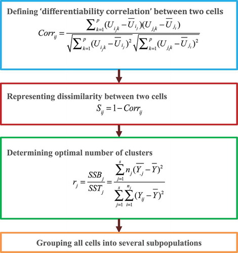
Step 1. Define a ‘differentiability correlation’ (Corr) between two cells based on differential expression patterns of genes in order to measure cell-cell similarities:

$Cor{r}_{ij}=\frac{{\sum }_{k=1}^p(U_{i_{j}k}-{\bar{U}}_{i_j})(U_{j_{i}k}-{\bar{U}}_{j_i})}{\sqrt{{\sum }_{k=1}^p(U_{i_{j}k}-{\bar{U}}_{i_j}{)}^2}\sqrt{{\sum }_{k=1}^p(U_{j_{i}k}-{\bar{U}}_{j_i}{)}^2}}$

where $U_{i_{j}k}$ represents the differential status of the $k\mathrm{t}\mathrm{h}$ gene in cell $i$:

$U_{i_{j}k}=\left\{\begin{array}{c}\begin{array}{cc}1,& k\in V_{i_j}^{+}\end{array}\\ \begin{array}{cc}-1,& k\in V_{i_j}^{-}\end{array}\\ \begin{array}{cc}0,& otherwise\end{array}\end{array}\right.$

$V_{{ }_{i_j}}^{+}$ (or $V_{{ }_{i_j}}^{-}$) denotes genes in the $i\mathrm{t}\mathrm{h}$ cell, and the expression level of each gene in $V_{{ }_{i_j}}^{+}$ (or $V_{{ }_{i_j}}^{-}$) are all larger (or smaller) than the average value across all other cells except the $j\mathrm{t}\mathrm{h}$ cell.

Step 2. The dissimilarity between two cells is calculated by

$S_{ij}=1-Cor{r}_{ij}$

Step 3. Determine the optimal number of clusters from the level that cell subpopulations are separated:

$r_j=\frac{SS{B}_j}{SS{T}_j}$

where $SSB=\sum _{j=1}^s{n}_j(\overline{Y_{.j}}-\bar{Y}{)}^2$ .

$SST=\sum _{j=1}^s\sum _{i=1}^{n_j}(Y_{ij}-\bar{Y}{)}^2$

$Y_{ij}$ represents the random response of the $i\mathrm{t}\mathrm{h}$ $(i=1,2,...,n_j)$ observation in the$j\mathrm{t}\mathrm{h}$ $(j=1,2,...,s)$ treatment group.

Step 4. Cells are grouped into several subpopulations based on hierarchical clustering.

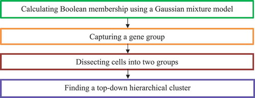
2.3.2.5. CellBIC

Kim et al. [26] investigated intrinsic multi-modality features of heterogeneous scRNA-seq data and presented a single-Cell BImodel Clustering (CellBIC) method to detect cellular subpopulations. CellBIC combines a top-down hierarchical clustering algorithm and a bimodal expression pattern of scRNA-seq data (Fig. 5).

Figure 5. Flowchart of single-cell bimodel clustering (CellBIC) method.

2.3.3. Consensus clustering

2.3.3.1. SC3

Kiselev et al. [27] developed a Single-Cell Consensus Clustering method (SC3). The robust method displayed high accuracy by combining multiple clustering techniques. SC3 is performed by the following six basic steps (Fig. 6).

Figure 6. Flowchart of single-cell consensus clustering method.

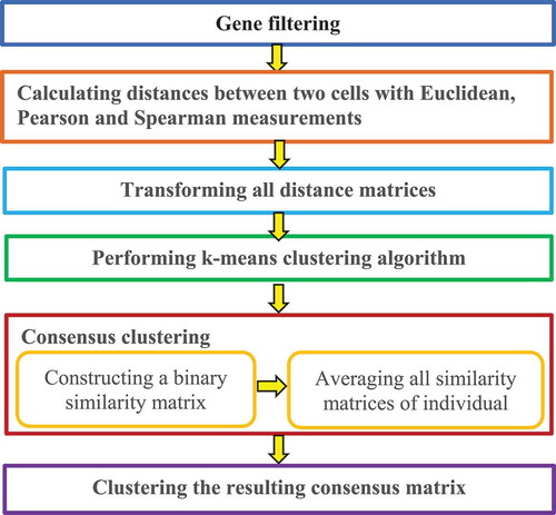
Step 1. Gene filtering.

Genes are removed that are either expressed in less than a% of cells or expressed in at least (100-a)% of cells, because these ubiquitous and rare genes, respectively, are not often informative for clustering.

Step 2. Distance calculation.

Distances are calculated between two cells using Euclidean, Pearson, and Spearman metrics.

Step 3. Transformation.

All distance matrices are transformed with PCA or the eigenvectors of the connected graph Laplacian matrix.

Step 4. K-means clustering.

A K-means clustering algorithm is applied on the first $d$ eigenvectors of the transformed distance matrices.

Step 5. Consensus clustering

A consensus matrix is calculated with a cluster-based similarity partitioning algorithm [57] via two steps. A binary similarity matrix is first constructed from cell labels for each individual K-means cluster result and all similarity matrices are then averaged for individual clustering results to obtain a consensus matrix. In the former, the SC3 similarity between the two cells is set as 1 if the two cells are clustered into the same subpopulation; otherwise, the similarity is set as 0.

Step 6. Hierarchical clustering.

The resulting consensus matrix is clustered using a hierarchical cluster method with complete agglomeration, followed by inference of the clusters at the $k$ level of hierarchy.

2.3.3.2. The SAFE-clustering method

Yang et al. [58] developed the SAFE-clustering method based on aggregated (from ensemble) clustering. The method comprises two components, with the first employing the SAFE-clustering of clustered scRNA-seq data using four state-of-the-art algorithms (SC3 [27], CIDR [24], Seurat [59] and tSNE+K-means). In the second component, SAFE-clustering performs cluster ensemble aggregation to obtain consensus cluster labels using three hypergraph-based partitioning methods (HGPA, MCLA, and CSPA). The details of the SAFE-clustering method are shown in the algorithm outlined below (Table 2), wherein ANMI represents the Average Normalized Mutual Information (ANMI) in the SAFE-clustering algorithm.

Table 2. The SAFE-clustering algorithm.

1: Run SC3, CIDR, Seurat and t-SNE+K-means to generate a $Y_{4\times n}$ matrix of cluster labels

2: Transform the output labels of each clustering method into a hypergraph

3: For $k=2$ to $K_{max}$//$K_{max}$ is either specified by the user or is the maximum value across these four individual methods

4: If MCLA = = TRUE

5: Do MCLA

6: Compute the Jaccard similarity matrix $S_{JAC}=\frac{{\mathrm{\hslash }}_p{\mathrm{\hslash }}_q^T}{{\mathrm{\hslash }}_p^2+{\mathrm{\hslash }}_q^2-{\mathrm{\hslash }}_p{\mathrm{\hslash }}_q^T}$ for two hyperedges ${\mathrm{\hslash }}_p$ and ${\mathrm{\hslash }}_q$

7: $k-\mathrm{w}\mathrm{a}\mathrm{y}$ partitioning using the $gpmetis$ program in the hMETIS package

8: Compute the association index ($M{C}_{ci}$), $c=1,2,...,k$, $i=1,2,...,n$, and assign each single cell to the meta-cluster $c$ with the largest $AI$ metric

9: If there are empty clusters

10: Re-label into $k^{\prime }$ non-empty meta-clusters

11: End

12: End

13: If HGPA = = TRUE

14: Do HGPA

15: $k-\mathrm{w}\mathrm{a}\mathrm{y}$ partitioning using the $sbmetis$ program in the hMETIS package

16: End

17: If CSPA = = TRUE

18: Do CSPA

19: Compute and normalize the similarity matrix $S$

20: $k-\mathrm{w}\mathrm{a}\mathrm{y}$ partitioning using the $gpmetis$ program in the hMETIS package

21: End

22: Calculate $ANMI$ across ensemble methods

23: Return consensus cluster labels ${\hat{L}}_e$ and $ANMI$

24: End

25: Return the optimal consensus result ${\hat{L}}_{e-opt}$ of ${\hat{k}}_{e-opt}$ clusters with the highest $ANMI$: $\text{({widehat L\_{e - opt}},{widehat K\_{e - opt}}) = mathop {arg max }}limits\_{{L\_e},{K\_e},m in { HGPA,MCA,and/orCSPA} } ANM{I\_m}}$

2.3.3.3. GiniClust2

Tsoucas and Yuan [60] developed a new computational model, GiniClust2, to identify rare and common cell types. GiniClust2 effectively combines the advantages of two complementary clustering algorithms including the Gini index-based technique and the Fano factor-based technique. The model assigns the more reliable subpopulations higher weights based on the following steps (Fig. 7).

Figure 7. Flowchart of method combining gini index and fano factor.

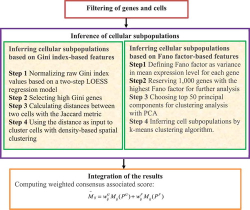
Step 1. Filter genes and cells by removing genes expressed in less than three cells, and cells with expression of less than 2,000 genes. GiniClust2 then performs the following four steps.

Step 2. Infer cell subpopulations based on the Gini index-based features.

In the Gini index-based clustering algorithm, GiniClust2 uses a two-step LOESS regression model and removes the trend with the maximum expression levels to normalize raw Gini index values. Genes with Gini index values significantly larger than zero after normalization are considered as high Gini value genes. The high Gini value genes are then used to calculate the distances between cells with the Jaccard metric. The distances are used to cluster cells with density-based spatial clustering.

Step 3. Infer cellular subpopulations based on Fano factor-based features.

The Fano factor-based clustering algorithm first defines the Fano factor as the variance in mean expression levels for each gene. The 1,000 genes with the highest Fano factor values are then reserved for further analysis. The top 50 principal components from principal components analysis (PCA) are then chosen for clustering analysis from the gene expression matrix. Finally, cellular subpopulations are inferred using the K-means clustering algorithm.

Step 4. Integrate the results from the Gini index-based method in Step 2 and the Fano factor-based method in Step 3 through a cluster-aware and a weighted consensus method to compute the probability that two cells belong to the same cluster.

$P^G$ and $P^F$ are the partitions obtained from the Gini index-based and Fano factor-based clustering algorithms, respectively. Each partition consists of cluster sets:

$C^G=\{C_1^G,C_2^G,...,C_{k_G}^G\}\mathrm{a}\mathrm{n}\mathrm{d}{C}^P=\{C_1^F,C_2^F,...,C_{k_F}^F\}.$

GiniClust2 defines the weighted consensus associated score as,

${\bar{M}}_{ij}=w_{ij}^G{M}_{ij}(P^G)+w_{ij}^F{M}_{ij}(P^F)$

where $M_{ij}(P^G)$and $M_{ij}(P^F)$denote the connectivity matrices:

$\begin{array}{rl}& M_{ij}(P^G)=\left\{\begin{array}{c}1,(i,j)\in C_k(P^G)\\ 0,otherwise\end{array}\right.\mathrm{a}\mathrm{n}\mathrm{d}\\ & M_{ij}(P^F)=\left\{\begin{array}{c}1,(i,j)\in C_k(P^F)\\ 0,otherwise\end{array}\right..\end{array}$

Connectivity between two cells is set as 1 if the two cells are grouped into the same cluster; otherwise, the value is set as 0.

and

$w_{ij}^G=\frac{w_{ij}^{G_{ini}}}{w_{ij}^{G_{ini}}+w_{ij}^{F_{ini}}}\mathrm{a}\mathrm{n}\mathrm{d}{w}_{ij}^{F_{ini}}=\frac{w_{ij}^{F_{ini}}}{w_{ij}^{G_{ini}}+w_{ij}^{F_{ini}}},$

where $w_{ij}^{G_{ini}}=max(w_i^{G_{ini}},w_j^{G_{ini}})$, $w_i^{G_{ini}}(x_i)$ denotes the cell-specific Gini index-based weights$w_i^{G_{ini}}(x_i)=1-1/(1+e^{\frac{x_i-{\mu }^{\prime }}{s^{\prime }}})$, $w_{ij}^{F_{ini}}=1-1/(1+e^{\frac{\mu -{\mu }^{\prime }}{s^{\prime }}})$, $x_i$ is the proportion by which cell $i$ belongs to the Gini index-based cluster, ${\mu }^{\prime }$ represents the proportion by which the Gini index-based and Fano factor-based clustering algorithms have effectively identical ability to find rare cell types, and $s^{\prime }$ denotes how quickly the Gini index-based clustering algorithm loses its ability to find rare cell types above ${\mu }^{\prime }$.

Step 5. Determine the final clustering assignment.

GiniClust2 builds the following non-negative matrix factorization model to produce a soft clustering,

$\underset{U}{min}||\bar{M}-U|{|}^2$

where $\bar{M}$ represents the probability that two cells belong to the same cluster. And an orthogonality constraint is used to obtain a hard clustering similar to K-means.

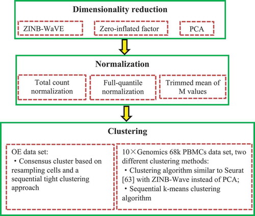
2.3.3.4. ZINB-WaVE

Risso et al. [61] developed the general and flexible model termed the Zero-Inflate Negative Binomial-based Wanted Variation Extraction (ZINB-WaVE) to represent single-cell data in low dimensionality while accounting for dropouts and over-dispersion (Fig. 8).

Figure 8. Flowchart of zero-inflate negative binomial-based wanted variation extraction.

ZINB-WaVE comprises the following steps.

For any$\pi \in [0,1]$, $\mu \ge 0$ and $\theta >0$, ZINB-WaVE is first defined as the probability mass function of the ZINB distribution by,

$f_{ZINB}(y;\mu ,\theta ,\pi )=\pi {\delta }_0(y)+(1-\pi )f_{NB}(y;\mu ,\theta )$

where ${\sigma }_0(\cdot )$ is the Dirac function, $f_{NB}(y;\mu ,\theta )=\frac{(y+\theta )}{(y+1)(\theta )}(\frac{\theta }{\theta +\mu }{)}^{\theta }(\frac{\mu }{\mu +\theta }{)}^y,\mathrm{\forall }y\in \mathrm{N}$.

Given $p$ genes (features) in $n$ cells (samples), $Y_{ij}$ represents the count of features $j$ in sample $i$. ZINB-WaVE is then modelled as $Y_{ij}$, representing a random variable following the ZINB distribution where the parameters are satisfied by the following regression models:

$\begin{array}{c}ln\left({\mu }_{ij}\right)={\left(X{\beta }_{\mu }+{\left(V{\gamma }_{\mu }\right)}^T+W{\alpha }_{\mu }+O_{\mu }\right)}_{ij}\\ \mathrm{l}\mathrm{o}\mathrm{g}\mathrm{i}\mathrm{t}\left({\pi }_{ij}\right)={\left(X{\beta }_{\pi }+{\left(V{\gamma }_{\pi }\right)}^T+W{\alpha }_{\pi }+O_{\pi }\right)}_{ij},\\ ln\left({\theta }_{ij}\right)={\varsigma }_j\end{array}$

where $\mathrm{l}\mathrm{o}\mathrm{g}\mathrm{i}\mathrm{t}(\pi )=ln(\pi /(1-\pi ))$, $X$ is a known $n\times M$ matrix corresponding to $M$ cell-level covariates, $V$ is a known $m\times L$ matrix corresponding to $m$ gene-level covariates, $W$ is an unknown $n\times K$ matrix corresponding to $K$ unknown cell-level covariates, $O_{\mu }$ and $O_{\pi }$ are known $n\text{timesm}$ matrices of offsets, and $\beta =({\beta }_{\mu },{\beta }_{\pi })$ is associated with $M\text{timesm}$ matrices of $X$ from regression parameters.

2.3.4. Other cluster methods

2.3.4.1. The SNN-clique algorithm

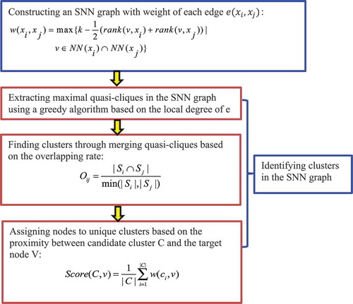
Xu et al. [62] developed the SNN-clique algorithm that combines shared nearest neighbour (SNN) and quasi-clique-based clustering models. The authors first established that the SNN method is relatively robust and can obtain stable performances, and then developed a quasi-clique-based clustering model to capture cell subpopulations with different shapes and densities (Fig. 9).

Figure 9. Flowchart of shared nearest neighbour (SNN) technique and quasi-clique-based clustering models.

2.3.4.2. ScImpute

Li W. V. and Li J. J. [63] introduced a statistical model, scImpute, that automatically detects possible dropouts and outlier cells. ScImpute comprises four steps (Fig. 10) as follows.

Figure 10. Flowchart of a new imputation model for scRNA-seq data.

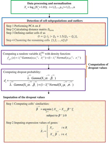
Step 1. Data processing and normalization.

ScImpute takes a count matrix, $X^C$, providing the expression values of $p$genes for $n$ cells as the input and first normalizes $X^C$ with the library size of each cell (sample) to obtain $X^N$. ScImpute then computes a matrix, $X$, to avoid infinite values in parameter estimation using the following model: .

$X_{ij}={log}_{10}(X_{{ }_{ij}}^N+1.01);i=1,2,\dots ,p,j=1,2,\dots ,n$

Step 2. Detect cell subpopulations and outliers.

ScImpute performs PCA on $X$ to achieve the ordination results, $Z$. The distance matrix $D_{n\times n}$ is then calculated from similarities within the $Z$dataset. For $L=\{l_1,l_2,..,l_n\}$, with $l_j$ representing the distance of cell $j$ to its nearest neighbour, ScImpute denotes its first and third quartiles as $Q_1$ and $Q_3$, respectively. The outlier cells $O$ are then defined as: $O=\{j:l_j>Q_3+1.5(Q_3-Q_1)\}$. Finally, ScImpute clusters the remaining cells $\{1,2,...,n\}\mathrm{\setminus }O$ into $K$ subpopulations with spectral clustering.

Step 3. Calculate dropout values.

ScImpute models the expression of gene $i$ in cell cluster $k$ as a random variable, $X_i^{(k)}$, with the density function as .

$f_{X_i^{(k)}}(x)={\lambda }_i^{(k)}Gamma(x;{\alpha }_i^{\left(k\right)},{\beta }_i^{(k)})+(1-{\lambda }_i^{(k)}Normal(x;{\mu }_i^{(\left.k\right)},{\sigma }_i^{(k)})$

The dropout probability by which gene $i$ in cell $j$ belongs to cluster $k$ can then be estimated as .

$d_{ij}=\frac{{\hat{\lambda }}_i^{(k)}Gamma(X_{ij};{\hat{\alpha }}_i^{(k)},\stackrel{(k)}{\underset{i}{\overset{\wedge }{\beta }}})}{{\hat{\lambda }}_i^{(k)}Gamma(X_{ij};{\hat{\alpha }}_i^{(k)},{\hat{\beta }}_i^{(k)})+(1-{\lambda }_i^{(k)}Normal(X_{ij};{\hat{\mu }}_i^{(k)},{\hat{\sigma }}_i^{(k)})}$

Step 4. Impute dropout values.

Gene set $A_j$ in cell $j$ requires imputation based on the threshold $t$ value of dropout probabilities: $A_j=\{i:d_{ij}\ge t\}$, whereas the gene set $B_j=\{i:d_{ij}<t\}$ has accurate gene expression data and does not require imputation. Given these assumptions, ScImpute first computes the similarities among cells based on the non-negative least squares from $B_j$:

$\text{eqalign{ \& {widehat beta \&{(j)}} = mathop {arg min }limits\_{{beta \&{(j)}}} ||{X\_{{B\_j},j}} - {X\_{{B\_j},{N\_j}}}{beta \&{(j)}}||\_2\&2 cr \& {rm{ subject to }}{beta \&{(j)}} ge 0, cr}}$

where $N_j$ denotes the indices of candidate neighbour cells of cell $j$. $\stackrel{(j)}{\stackrel{\wedge }{\beta }}$ is then used to impute the expression values of genes in $A_j$ from cell $j$ based on the expression of the same genes in other similar cells from $B_j$:

${\hat{X}}_{ij}=\left\{\begin{array}{c}{X}_{ij},i\in B_j\\ X_{i,N_j}{\hat{\beta }}^{(j)},i\in A_j\end{array}\right..$

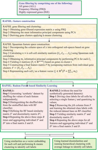
2.3.4.3. RAFSIL

Pouyan et al. [64] exploited a random forest-based method, RAFSIL, to identify similarities among cells via clustering of scRNA-seq data using the following three steps.

Step 1. Use three types of filtering based on gene abundances: all genes (ALL), frequency filtering (FRQ), and highly expressed genes (HiE).

Step 2. Use FRQ to filter and cluster genes by treating genes as observations and cells as features. The most representative principal components via PCA are then chosen for further analysis.

Step 3. Classification of all cells using a random forest-based similarity learning method (Fig. 11).

Figure 11. Flowchart of random forest-based single-cell clustering method.

2.3.4.4. SparseDC

Barron et al. [65] hypothesized that cell types changed when micro-environments changed and designed the Sparse Differential Clustering (SparseDC) algorithm to evaluate these dynamics. SparseDC defines ‘condition A’ and ‘condition B’ as the conditions before and after the change, respectively. The gene expression matrix $X_{p\times n}$ represents the expression of $p$ genes in $n$ cells under condition A. $C_k$indicates the indices of all cells contained in cluster $k$ under condition A, $j\in C_k$indicates that cell $j$ in condition A is grouped into cluster $k$, $j=1,2,...,n,k=1,2,...,K$. In addition, $N_k$ is the size of $C_k$ with ${\sum }_{k=1}^K{N}_k=n$, $\mu {\hspace{0.17em}}_{ik}$ as the cluster centre for gene $i$ and cluster $k$ under condition A. $X^{\prime },C_k^{\prime },N_k^{\prime },{\mu }_{ik}^{\prime }$ can similarly be defined for condition B.

SparseDC then exploits the following optimization problem:

$\text{matrix{ {min T(C,C',mu ,mu ') = mathop sum limits\_{i = 1}^p mathop sum limits\_{k = 1}^K { {1 over 2}mathop sum limits\_{j in {C\_k}} {{({X\_{ij}} - {mu \_{ik}})}^2} + {1 over 2}mathop sum limits\_{j in {C\_k}} {{({{X'}\_{ij}} - {{mu '}\_{ik}})}^2}} cr + sqrt {{N\_k}} {lambda \_1}left| {{mu \_{ik}}} right| + sqrt {{{N'}\_k}} {lambda \_1}left| {{{mu '}\_{ik}}} right| cr ,+ (sqrt {{N\_k}} + sqrt {{{N'}\_k}} ){lambda \_2}left| {{mu \_{ik}} - {{mu '}\_{ik}}} right|} ,} cr }}$

where ${\lambda }_1$ and ${\lambda }_2$ are parameters.

SparseDC initializes $C$ and $C^{\prime }$ by randomly assigning each cell to clusters and then detecting the final clusters by iteratively updating {C,C’} and $\{\mu ,{\mu }^{\prime }\}$ until the clustering results do not change.

2.3.4.5. ScNN

Lin et al. [66] designed a neural network-based (scNN) method to detect and analyse cellular clusters. Given that the vector $x^{(0)}$ is the input of the scNN algorithm and $x^{(i)}$ is the output of $i\mathrm{t}\mathrm{h}$ hidden layer, scNN explores the following forward propagation:

$x^{(i)}=a(W^{(i)}{x}^{(i-1)}+b^{(i-1)}),$

where $a$ is the activation function, $b$ is an intercept term, and $W$ is the weight matrix. scNN uses the tangent (tanh) as the activation function due to its optimal performance and subsequently focuses on learning $W$ and $b$: .

$tanh(x)=\frac{1-exp(-2x)}{1+exp(-2x)}$

For the output layer, scNN uses a softmax activation function to conduct discrete classification:

$output(x)=softmax(x)={\left[\frac{exp(x_1)}{{\sum }_{c}exp(x_c)}\cdots \frac{exp(x_C)}{{\sum }_{c}exp(x_c)}\right]}^T,$

where $C$ denotes the indices of all cell types in the training dataset.

The output $f(x^{(0)}{)}_c$ for each node $c$ in the output layer indicates the probability by which the sample $x^{(0)}$ in the input layer belongs to cell type $c$:

$f(x^{(0)}{)}_c=p(y=c|x^{(0)}).$

2.3.4.6. ScVDMC

Zhang et al. [67] exploited a Variance-Driven Multitask-based Clustering (scVDMC) algorithm to solve the cross-cell-population clustering problem. scVDMC utilizes multiple single-cell populations from different datasets and identifies cell clusters by controlling the variance among their subpopulations within each dataset and across all datasets.

scVDMC assumes that the matrix $X^{(d)}\in {\mathbb{R}}^{p\times n^{(d)}}$ indicates gene expression values of scRNA-seq from domain $d\in \{1,2,...D\}$, where each domain, $d$, represents a single-cell population for clustering, $p$ is the number of genes (features) and $n^{(d)}$ is the size of single-cell samples from domain $d$. $U^{(d)}\in {\mathbb{R}}^{p\times k}$ denotes the centres of clusters (cell types), vector $Y^{i,j}=[U_{i,j}^{(1)},U_{i,j}^{(2)},...,U_{i,j}^{(D)}{]}^T$ represents the $(i,j)-th$ entry of every $U^{(d)}$, and $V^{(d)}\in \{0,1{\}}^{n^{(d)}\times k}$ indicates the assignments of each single cell into clusters while $k$ is the number of clusters. $B\in \{0,1{\}}^p$ represents the indicators of feature selection where $B_i$ is set as 1 if the $i\mathrm{t}\mathrm{h}$ gene is selected as a feature, and set as 0 otherwise. $D_B$ is the diagonal matrix on $B$. scVDMC then defines the following optimization model:

$\underset{U^{(d)},V^{(d)},B}{min}\frac{1}{2}\sum _{d=1}^D||D_B(X^{(d)}-U^{(d)}{V}^{{(d)}^T})|{|}_F^2-w\sum _{d=1}^D{B}^{T}Var(U^{(d)})+\alpha {\sum }_{i,j}{B}_{i}Var(Y^{(i,j)})$

$\mathrm{s}\mathrm{u}\mathrm{b}\mathrm{j}\mathrm{e}\mathrm{c}\mathrm{t}\mathrm{t}\mathrm{o}\sum B=\lambda ,$

$\sum _j{V}_{i,j}^{(d)}=1,\mathrm{\forall }i=1,2,\dots ,n^{(d)},\mathrm{\forall }d=1,2,\dots ,D.$

Zhang et al. [67] solved the optimization problem using an alternating updating strategy, thereby addressing the cross-population clustering problem.

2.4. Evaluation metrics

To evaluate clustering methods, several popular metrics can be used including the Adjusted Rand Index (ARI) and the Normalized Mutual Information (NMI) metrics based on known labels of single cells.

2.4.1. ARI

Given that $n$ cells are grouped into $k$ clusters, $\{u_i{\}}_{i=1}^n$ represents the inferred cluster labels, and $\{v_i{\}}_{i=1}^n$ is the pre-annotated labels. Then,

$\text{ARI = {{sumnolimits\_{ls} {left({matrix{ {{n\_{ls}}} cr 2 cr } } right) - left(sumnolimits\_l {left(matrix{ {{n\_l}} cr 2 cr } right)} sumnolimits\_s {left(matrix{ {{n\_s}} cr 2 cr } right)} right)}/left(matrix{ ncr 2 cr }right )} over {left(sumnolimits\_l {left(matrix{ {{n\_l}} cr 2 cr } right)} + sumnolimits\_s {left(matrix{ {{n\_s}} cr 2 cr } right)} right)/2 - left(sumnolimits\_l {left(matrix{ {{n\_l}} cr 2 cr } right)} sumnolimits\_s {left(matrix{ {{n\_s}} cr 2 cr } right)} )/left(matrix{ ncr 2 cr } right)}}}$

where $l$ and $s$ denote the $k$ clusters, $n_l={\sum }_i^{n}I(u_i=l)$, $n_s={\sum }_i^{n}I(v_i=s)$, and $n_{ls}={\sum }_{i,j}^{n}I(u_i=l)I(v_i=s)$with $I(x=y)$ as an indicator function with value of 1 for $x=y$, but 0 otherwise. The ARI decreases with increasing disagreement between the inferred labels and the known labels, with a value of 1 when the inferred labels perfectly coincide with the known labels.

2.4.2. NMI

Given that $p_l=\frac{n_l}{n}$, $q_s=\frac{n_s}{n}$, and $z_{ls}=\frac{n_{ls}}{n}$, then $\mathrm{\hslash }(u)=-{\sum }_l{p}_{l}log(p_l)$and $\mathrm{\hslash }(v)=-{\sum }_s{q}_{s}log(q_s)$ are the entropies of the two subpopulations, respectively, and $i(u,v)={\sum }_{l,s}{z}_{ls}log(z_{ls}/p_l/q_s)$ is their mutual information. The NMI is used to measure the level of perfect overlap between subpopulations, and also decreases with increasing disagreement between the inferred and known labels. The NMI is defined as:

$NMI=i(u,v)/\sqrt{\mathrm{\hslash }(u)\mathrm{\hslash }(v)}$

3. Results

scRNA-seq technologies allow numerous avenues for revealing novel and potentially unexpected biological discoveries. For example, scRNA-seq has been used to capture subclones via transcriptomic comparisons of neoplastic cells. The strategy holds enormous prospects for applied and basic biology, including clinical trials [23]. scRNA-seq clustering aims to elucidate cell-to-cell heterogeneity and uncover cell subgroups and cell dynamics at the group level. More importantly, scRNA-seq clustering analysis can allow the discovery of new subtypes of cells and marker genes for existing cell types.

Two aspects of scRNA-seq data analysis were discussed in the present review: relevant datasets and analytical tools. In particular, we discussed scRNA-seq clustering models including K-means clustering, hierarchical clustering, consensus clustering, and other similar methods. Two primary evaluation metrics (e.g. ARI and NMI) were used to evaluate these methods.

We performed extensive experiments to evaluate the performances of seven state-of-the-art scRNA clustering methods on five public available datasets. These seven methods are CIDR [24], SC3 [27], tSNE+k-means (tSNE [68] followed by k-means clustering), RaceID [53], scImpute [63], SAFE [58], and GiniClust2 [61], respectively. These five datasets are from human brain [69], cerebral cortex [70], IPF [71], peripheral blood mononuclear cells [58], and mouse 2-cell and 4-cell embryos [72], respectively. They can be downloaded from the GEO or SRA database (GSE67835, SRP041736, GSE86618, SRP073767 and GSE57249). The experiments were performed on an iMAC with 2.4 GHz Inter Core i5, 8GB 2133 MHz CPDDR3 of RAM and OS Catalina 10.15.2 operating system.

We preprocessed scRNA-seq data based on the preprocessing steps provided by the corresponding papers. The results are shown in Table 3. In the human brain dataset [69], samples with library size more than 10,000 were retained. In the cerebral cortex dataset [70], genes expressed in less than 2 cells were removed. In the peripheral blood mononuclear cells [58] and mouse 2-cell and 4-cell embryos [72] datasets, the raw tag table were normalized by size factor and transformed by ${log}_{10}\left(X+1\right)$. In the human IPF dataset [71], each expression profile was transformed by z-scores (${z^s}_{ij}=\frac{({E^s}_{ij}-{{\mu }^s}_i)}{{{\sigma }^s}_i}$, where ${{\sigma }^s}_i$ and ${{\mu }^s}_i$ represent the standard and mean deviation, respectively). The results of comparison were shown in Table 4–8.

Table 3. The summary statistics of the five scRNA-seq datasets after preprocessing.

Dataset	Cell types	Cells	Genes
human brain	8	420	21,517
human cerebral cortex	11	300	8,686
human IPF	9	540	56,650
peripheral blood mononuclear cells	3	500	32,738
2-cell and 4-cell mouse embryos	3	49	25,737

Table 4. The performance comparison of seven methods on the human brain dataset.

Method	ARI	NMI	Runtime
CIDR	0.8977	0.9467	6.95 s
SC3	0.7985	0.9921	1.95 min
tSNE+k-means	0.8408	0.8249	30.35 s
RaceID	0.5029	0.8003	1.47 min
scImpute	0.5541	0.7388	2.60 min
SAFE	0.6498	0.7618	2.40 min
GiniClust2	0.9121	0.9492	39.71s

Table 5. The performance comparison of seven methods on the human cerebral cortex dataset.

Method	ARI	NMI	Runtime
CIDR	0.7374	0.4469	2.43 s
SC3	0.8933	1.0	53.55 s
tSNE+k-means	0.8897	1.0	48.10s
RaceID	0.5649	0.2199	1.32 min
scImpute	0.7548	1.0	1.40 min
SAFE	0.6689	0.5950	59.97s
GiniClust2	0.5819	0.7754	22.14s

Table 6. The performance comparison of seven methods on the human IPF dataset.

Method	ARI	NMI	Runtime
CIDR	0.2183	0.3917	12.01 s
SC3	0.7096	0.9820	3.51 min
tSNE+k-means	0.1736	0.4591	46.33 s
RaceID	0.1009	0.2852	4.99 min
scImpute	0.2930	0.7702	13.62 min
SAFE	0.2187	0.4375	4.66 min
GiniClust2	0.4871	0.9370	2.06 min

Table 7. The performance comparison of seven methods on the peripheral blood mononuclear cells dataset.

Method	ARI	NMI	Runtime
CIDR SC3	0.9210 0.8546	0.9752 0.9446	8.11 s 2.71 mins
tSNE+k-means	0.9884	0.9871	20.83 s
RaceID	0.8386	0.0933	57.77 s
scImpute	0.9826	0.9628	1.88 min
SAFE	0.8920	0.9136	3.27 min
GiniClust2	0.9826	0.9814	29.12 min

Table 8. The performance comparison of seven methods on the 2-cell and 4-cell mouse embryos dataset.

Method	ARI	NMI	Runtime
CIDR	0.8606	0.9114	2.03 s
SC3	0.9483	0.9114	21.90 s
tSNE+k-means	1.0	1.0	2.31 s
RaceID	0.1268	0.9114	13.32 s
scImpute	1.0	0.9114	54.19 s
SAFE	0.7731	0.6877	24.07 s
GiniClust2	0.9483	0.9114	16.45 s

In the human brain scRNA-Seq dataset [69], GiniClust2 obtained an ARI of 0.9121 and can correctly identify most cells for each cell type. SC3 obtained the best NMI of 0.9921 (Table 4). In the human cerebral cortex scRNA-Seq dataset [70], SC3 had the highest score of ARI, and was followed by tSNE+k-means. SC3, tSNE+k-means and scImpute achieved the best results in terms of NMI. But tSNE+k-means (48.10 secs) was faster than SC3 (53.55 secs) (Table 5). In the human IPF scRNA-Seq dataset [71], SC3 achieved the best performances on both ARI and NMI, which were far better than other methods (Table 6). In the peripheral blood mononuclear cells scRNA-Seq dataset [58], these seven methods obtained better performances. tSNE+k-means obtained the best performances on both ARI and NMI (Table 7). In the 2-cell and 4-cell mouse embryos scRNA-Seq dataset [72], tSNE+k-means obtained the best performances (1.0) on both ARI and NMI. More importantly, CIDR was the fastest on these five scRNA-seq datasets (Table 8). The experimental results from these five dataseets shows that CIDR usually has the least runtime, and SC3 and tSNE+k-means usually have better clustering accuracy.

4. Discussion and further research

Current computational models for clustering scRNA-seq data effectively identified cellular subpopulations, however, they have a number of challenges encapsulated within the seven following categories.

4.1. Lacking gold-standard benchmark datasets

scRNA-seq technologies have rapidly developed, and scRNA-seq clustering techniques have efficiently been able to capture cell subpopulations. However, the lack of gold-standard benchmark datasets severely limits systematic comparisons of performance of various clustering algorithms. Thus, integrating existing experimental data and generating single-cell dataset benchmarks may be a major challenge for advancing single-cell data analysis [10,73,74].

4.2. Identifying a cluster number

Almost all clustering algorithms require a parameter for the number of desired clusters. Indeed, the parameter has important effects on clustering outcomes. Although RaceID [53], SNN-cliq [62], and SC3 [27] provide estimations of cluster numbers, $K$, these methods have other limitations. RaceID [53] performs poorly when no rare cell types are present, while SNN-cliq [62] and SC3 [27] have high complexity and are not scalable. Consequently, selecting an appropriate cluster parameter is a challenging task.

4.3. Reclustering cell subpopulations

Many algorithms (e.g., RaceID [53] and GiniClust2 [60]) exhibit good performances when clusters are roughly equal in size. Unfortunately, decreased performance in identifying rare cell types occurs when more frequent cell types are clustered. To solve this problem, many solutions have used a divide-and-conquer technique to recluster large cell populations after an initial clustering [75,76,]. However, a critical problem arises with regard to how to determine whether a large cell subpopulation should be reclustered [22].

4.4. Dimension reduction

scRNA-seq dataset components contain abundant cells. While it is feasible to cluster these large datasets, visualizing and interpreting these results remains a challenge. Linear dimensional reduction techniques (e.g., PCA) can not accurately uncover potential associations between cells due to dropout and noise. In contrast, nonlinear dimensional reduction strategies (e.g., t-SNE [52,68,77,,] and UMAP [77]) can produce outcomes that are easier to interpret. However, they incorporate parameters requiring manual adjustment, and this severely affects visualization. Thus, using an appropriate method for choosing parameters to perform dimensional reduction in scRNA-seq clustering is an unsolved problem [22].

4.5. Validation and visualization of clustering results

The validation of scRNA-seq clustering results may be one of the most pressing challenges in analysing these data. The currently optimal validation method is to confirm cell types by other methods like screening cells from different cell lines [70] or during the first stages of embryonic development [78], or by evaluating tissues that are well studied (e.g., peripheral blood mononuclear cells) [58]. These cell types or tissues can serve as useful ground-truthing benchmarks but are, however, unlikely to be complex, and there are also limited tissue examples [22]. In addition, there are numerous analysis tools for identifying gene enrichment analysis tools, but tools to analyse cell type enrichment are scarce. Consequently, exploiting visualization tools to identify cell type enrichments may be a promising area of alternative research.

4.6. Ensemble clustering

Experiments have confirmed that no individual scRNA-seq clustering algorithm can capture true clusters and achieve optimal performance in all situations. For example, SC3 [27], SINCERA [55], and pcaReduce [79] performed better than other models in the dataset investigated in Biase et al. [72]. In contrast, tSNE+k-means and SC3 [27] exhibited more robust performances when analysing the dataset provided by Klein et al. [27,80,]. Ensemble clustering produces several clustering results for a given dataset and identifies final solutions based on the associations observed across the ensemble. The solutions from ensemble clustering are more stable and robust than every individual solution within the ensemble. Consequently, it may be an important area of future research to leverage ensemble clustering to integrate gene expression data from all individual cells and diverse clustering methods given that individual clustering algorithms are less likely to achieve as optimal of performances.

4.7. Personalized medicine

More extensive research into individual cellular dynamics can increase our understanding of the developmental processes and pathogenesis mechanisms of various complex diseases. These findings can then be effectively applied in personalized medicine and contribute to the development of the field. For example, scRNA-seq clustering has been used to identify intra-tumoural heterogeneity [73,81–84] and cluster tumour cell subpopulations [85,86,]. Nevertheless, the application of these methods in adult somatic stem cell research is currently restricted due to limited knowledge about individual stem cells [86–89]. Thus, a significant challenge of the field may be to design novel statistical quantification techniques to detect cell subpopulations and design personalized treatment options for individual patients.

Acknowledgments

We would like to thank all authors of the cited references.

Disclosure statement

Authors Geng Tian and Jialiang Yang were employed by the company Geneis (Beijing) Co. Ltd. The remaining authors declare that the research was conducted in the absence of any commercial or financial relationships that could be construed as a potential conflict of interest.

Additional information

Funding

This research was funded by the Natural Science Foundation of China (Grant 61803151), the Natural Science Foundation of Hunan province (Grant 2018JJ2461, 2018JJ3570), and the Project of Scientific Research Fund of Hunan Provincial Education Department (Grant 17A052).

References

- Kester L, van Oudenaarden A. Single-cell transcriptomics meets lineage tracing. Cell Stem Cell. 2018;23(2):166–179.
- Renardy M, Jilkine A, Shahriyari L, et al. Control of cell fraction and population recovery during tissue regeneration in stem cell lineages. J Theor Biol. 2018;445:33–50.
- Karaayvaz M, Cristea S, S M G, et al. Unravelling subclonal heterogeneity and aggressive disease states in TNBC through single-cell RNA-seq. Nat Commun. 2018;9(1):3588.
- Zheng H, Pomyen Y, M O H, et al. Single-cell analysis reveals cancer stem cell heterogeneity in hepatocellular carcinoma. Hepatology. 2018;68(1):127–140.
- Bartoschek M, Oskolkov N, Bocci M, et al. Spatially and functionally distinct subclasses of breast cancer-associated fibroblasts revealed by single cell RNA sequencing. Nat Commun. 2018;9(1):5150.
- J A F, Wang Y, Riesenfeld SJ, et al. Single-cell reconstruction of developmental trajectories during zebrafish embryogenesis. Science. 2018 ;360(979):eaar3131
- Raj B, D E W, McKenna A, et al. Simultaneous single-cell profiling of lineages and cell types in the vertebrate brain. Nat Biotechnol. 2018;36(5):442.
- Q H N, Pervolarakis N, Blake K, et al. Profiling human breast epithelial cells using single cell RNA sequencing identifies cell diversity. Nat Commun. 2018;9(1):2028.
- Kumar MP, Du J, Lagoudas G, et al. Analysis of single-cell RNA-seq identifies cell-cell communication associated with tumor characteristics. Cell Rep. 2018;25(6):1458–1468. e4.
- Tian L, Dong X, Freytag S, et al. Benchmarking single cell RNA-sequencing analysis pipelines using mixture control experiments. Nat Methods. 2019;16(1).
- Stuart T, Satija R. Integrative single-cell analysis. Nature reviews genetics. 2019;20(5):257–272.
- Shema E, Bernstein BE, Buenrostro JD. Single-cell and single-molecule epigenomics to uncover genome regulation at unprecedented resolution. Nat Genet. 2018;51(1).
- Jia G, Preussner J, Chen X, et al. Single cell RNA-seq and ATAC-seq analysis of cardiac progenitor cell transition states and lineage settlement. Nat Commun. 2018;9(1):4877.
- Tiklová K, Å K B, Lahti L, et al. Single-cell RNA sequencing reveals midbrain dopamine neuron diversity emerging during mouse brain development. Nat Commun. 2019;10(1):581.
- Birnbaum KD. Power in numbers: single-cell RNA-seq strategies to dissect complex tissues. Annu Rev Genet. 2018;52:203–221.
- M W E J F, Minnoye L, Aibar S, et al. Mapping gene regulatory networks from single-cell omics data. Brief Funct Genomics. 2018;17(4):246–254.
- Packer J, Trapnell C. Single-cell multi-omics: an engine for new quantitative models of gene regulation. Trends Genet. 2018;34(9):653–665.
- Butler A, Hoffman P, Smibert P, et al. Integrating single-cell transcriptomic data across different conditions, technologies, and species. Nat Biotechnol. 2018;36(5):411.
- Haghverdi L, A T L L, M D M, et al. Batch effects in single-cell RNA-sequencing data are corrected by matching mutual nearest neighbors. Nat Biotechnol. 2018;36(5):421.
- Lambrechts D, Wauters E, Boeckx B, et al. Phenotype molding of stromal cells in the lung tumor microenvironment. Nat Med. 2018;24(8):1277.
- Andor N, E F S, D K C, et al. Single-cell RNA-Seq of follicular lymphoma reveals malignant B-cell types and coexpression of T-cell immune checkpoints. Blood. 2019;133(10):1119–1129.
- Kiselev VY, Andrews TS, Hemberg M. Challenges in unsupervised clustering of single-cell RNA-seq data. Nat Rev Genet. 2019;20(1).
- Qi R, Ma A, Ma Q, et al. Clustering and classification methods for single-cell RNA-sequencing data. Brief Bioinform. 2019;7:1–3.
- Lin P, Troup M, Ho JWK. CIDR: ultrafast and accurate clustering through imputation for single-cell RNA-seq data. Genome Biol. 2017;18(1):59.
- Jiang H, Sohn L, Huang H, et al. Single cell clustering based on cell-pair differentiability correlation and variance analysis. Bioinformatics. 2018;34:3684–3694.
- Kim J, D E S, Won KJ. CellBIC: bimodality-based top-down clustering of single-cell RNA sequencing data reveals hierarchical structure of the cell type. Nucleic Acids Res. 2018;46(21):e124–e124.
- V Y K, Kirschner K, M T S, et al. SC3-consensus clustering of single-cell RNA-Seq data. Nat Methods. 2017;14(5):483–486.
- Trapnell C, Cacchiarelli D, Grimsby J, et al. The dynamics and regulators of cell fate decisions are revealed by pseudotemporal ordering of single cells. Nat Biotechnol. 2014;32(4):381.
- Petropoulos S, Edsgärd D, Reinius B, et al. Single-cell RNA-seq reveals lineage and X chromosome dynamics in human preimplantation embryos. Cell. 2016;165(4):1012–1026.
- Yan L, Yang M, Guo H, et al. Single-cell RNA-Seq profiling of human preimplantation embryos and embryonic stem cells. Nat Struct Mol Biol. 2013;20(9):1131.
- Goolam M, Scialdone A, S J L G, et al. Heterogeneity in Oct4 and Sox2 targets biases cell fate in 4-cell mouse embryos. Cell. 2016;165(1):61–74.
- A A K, J K K, J C H T, et al. Single cell RNA-sequencing of pluripotent states unlocks modular transcriptional variation. Cell Stem Cell. 2015;17(4):471–485.
- Treutlein B, D G B, A R W, et al. Reconstructing lineage hierarchies of the distal lung epithelium using single-cell RNA-seq. Nature. 2014;509(7500):371.
- Ting D T, Wittner B S, Ligorio M, et al. Single-cell RNA sequencing identifies extracellular matrix gene expression by pancreatic circulating tumor cells. Cell Rep. 2014;8(6):1905–1918.
- A P P, Tirosh I, J J T, et al. Single-cell RNA-seq highlights intratumoral heterogeneity in primary glioblastoma. Science. 2014;344(6190):1396–1401.
- Usoskin D, Furlan A, Islam S, et al. Unbiased classification of sensory neuron types by large-scale single-cell RNA sequencing. Nat Neurosci. 2015;18(1):145.
- A M K, Mazutis L, Akartuna I, et al. Droplet barcoding for single-cell transcriptomics applied to embryonic stem cells. Cell. 2015;161(5):1187–1201.
- Zeisel A, A B M-M, Codeluppi S, et al. Cell types in the mouse cortex and hippocampus revealed by single-cell RNA-seq. Science. 2015;347(6226):1138–1142.
- Deng Q, Ramsköld D, Reinius B, et al. Single-cell RNA-seq reveals dynamic, random monoallelic gene expression in mammalian cells. Science. 2014;343(6167):193–196.
- S A M, J C L, X Z M, et al. Single cell RNA sequencing of human liver reveals distinct intrahepatic macrophage populations. Nat Commun. 2018;9(1):4383.
- Shekhar K, S W L, I E W, et al. Comprehensive classification of retinal bipolar neurons by single-cell transcriptomics. Cell. 2016;166(5):1308–1323. e30.
- J M Z, Fan J, H C F, et al. An interpretable framework for clustering single-cell RNA-Seq datasets. BMC Bioinformatics. 2018;19(1):93.
- Li J, Smalley I, M J S, et al. SinCHet: a MATLAB toolbox for single cell heterogeneity analysis in cancer. Bioinformatics. 2017;33(18):2951–2953.
- D J M, K R C, A T L L, et al. Scater: pre-processing, quality control, normalization and visualization of single-cell RNA-seq data in R. Bioinformatics. 2017;33(8):1179–1186.
- Weinreb C, Wolock S, Klein AM. SPRING: a kinetic interface for visualizing high dimensional single-cell expression data. Bioinformatics. 2017;34(7):1246–1248.
- Gardeux V, F P A D, Shajkofci A, et al. ASAP: a web-based platform for the analysis and interactive visualization of single-cell RNA-seq data. Bioinformatics. 2017;33(19):3123–3125.
- Wang B, Ramazzotti D, De Sano L, et al. SIMLR: A tool for large‐scale genomic analyses by multi‐kernel learning. Proteomics. 2018;18(2):1700232.
- F A W, Angerer P, Theis FJ. SCANPY: large-scale single-cell gene expression data analysis. Genome Biol. 2018;19(1):15.
- Ji Z, TSCAN: JH. Pseudo-time reconstruction and evaluation in single-cell RNA-seq analysis. Nucleic Acids Res. 2016;44(13):e117–e117.
- DeTomaso D, Yosef N. FastProject: a tool for low-dimensional analysis of single-cell RNA-Seq data. BMC Bioinformatics. 2016;17(1):315.
- Zhu X, T K W, Tasato A, et al. Granatum: a graphical single-cell RNA-Seq analysis pipeline for genomics scientists. Genome Med. 2017;9(1):108.
- G C L, Rachh M, J G H, et al. Fast interpolation-based t-SNE for improved visualization of single-cell RNA-seq data. Nat Methods. 2019;16(3):243.
- Grün D, Lyubimova A, Kester L, et al. Single-cell messenger RNA sequencing reveals rare intestinal cell types. Nature. 2015;525(7568):251.
- Chlis NK, Alexander WF, Theis FJ. Model-based branching point detection in single-cell data by K-branches clustering. Bioinformatics. 2017;33:20.
- Guo M, Wang H, S S P, et al. SINCERA: a pipeline for single-cell RNA-Seq profiling analysis. PLoS Comput Biol. 2015;11(11):e1004575.
- Prabhakaran S, Azizi E, Carr A, et al. Dirichlet process mixture model for correcting technical variation in single-cell gene expression data. International conference on machine learning; Hongkong; 2016. p. 1070–1079.
- Strehl A, Ghosh J. Cluster ensembles — a knowledge reuse framework for combining multiple partitions. JMLR.org. 2003;3:583—617.
- Yang Y, Huh R, Culpepper HW, et al. SAFE-clustering: single-cell aggregated (from ensemble) clustering for single-cell rna-seq data. In: bioRxiv. 2018. p. 215723.
- Satija R, J A F, Gennert D, et al. Spatial reconstruction of single-cell gene expression data. Nat Biotechnol. 2015;33(5):495.
- Tsoucas D, Yuan GC. GiniClust2: a cluster-aware, weighted ensemble clustering method for cell-type detection. Genome Biol. 2018;19(1):58.
- Risso D, Perraudeau F, Gribkova S, et al. A general and flexible method for signal extraction from single-cell RNA-seq data. Nat Commun. 2018;9(1):284.
- Xu C, Su Z. Identification of cell types from single-cell transcriptomes using a novel clustering method. Bioinformatics. 2015;31(12):1974–1980.
- W V L, Li JJ. An accurate and robust imputation method scImpute for single-cell RNA-seq data. Nat Commun. 2018;9(1):997.
- M B P, Kostka D. Random forest based similarity learning for single cell RNA sequencing data. Bioinformatics. 2018;34(13):i79–i88.
- Barron M, Zhang S, Li J. A sparse differential clustering algorithm for tracing cell type changes via single-cell RNA-sequencing data. Nucleic Acids Res. 2017;46(3):e14–e14.
- Lin C, Jain S, Kim H, et al. Using neural networks for reducing the dimensions of single-cell RNA-Seq data. Nucleic Acids Res. 2017;45(17):e156–e156.
- Zhang H, C A A L, Li Z, et al. A multitask clustering approach for single-cell RNA-seq analysis in recessive dystrophic epidermolysis bullosa. PLoS Comput Biol. 2018;14(4):e1006053.
- Maaten L, Hinton G. Visualizing data using t-SNE. J Mach Learn Res. 2008;9(Nov):2579–2605.
- Darmanis S, Sloan SA, Zhang Y, et al. A survey of human brain transcriptome diversity at the single cell level. Proceedings of the National Academy of Sciences. 2015; 112(23):7285–7290.
- A A P, T J N, Shuga J, et al. Low-coverage single-cell mRNA sequencing reveals cellular heterogeneity and activated signaling pathways in developing cerebral cortex. Nat Biotechnol. 2014;32(10):1053.
- Xu Y, Mizuno T, Sridharan A, et al. Single-cell RNA sequencing identifies diverse roles of epithelial cells in idiopathic pulmonary fibrosis. JCI Insight. 2016;1:20.
- F H B, Cao X, Zhong S. Cell fate inclination within 2-cell and 4-cell mouse embryos revealed by single-cell RNA sequencing. Genome Res. 2014;24(11):1787–1796.
- Barkas N, Petukhov V, Nikolaeva D, et al. Joint analysis of heterogeneous single-cell RNA-seq dataset collections. Nat Methods. 2019;16(8):695–698.
- McGinnis CS, Patterson DM, Winkler J, et al. MULTI-seq: sample multiplexing for single-cell RNA sequencing using lipid-tagged indices. Nat Methods. 2019;16(1).
- A C V, Satija R, Reynolds G, et al. Single-cell RNA-seq reveals new types of human blood dendritic cells, monocytes, and progenitors. Science. 2017;356(6335):eaah4573.
- J N C, E Z M, Fenselau H, et al. A molecular census of arcuate hypothalamus and median eminence cell types. Nat Neurosci. 2017;20(3):484.
- Becht E, McInnes L, Healy J, et al. Dimensionality reduction for visualizing single-cell data using UMAP. Nat Biotechnol. 2019;37(1):38.
- Fan X, Zhang X, Wu X, et al. Single-cell RNA-seq transcriptome analysis of linear and circular RNAs in mouse preimplantation embryos. Genome Biol. 2015;16(1):148.
- Yau C. pcaReduce: hierarchical clustering of single cell transcriptional profiles. BMC Bioinformatics. 2016;17(1):140.
- Ronan T, Anastasio S, Qi Z, et al. Openensembles: a python resource for ensemble clustering. J Mach Learn Res. 2018;19(1):956–961.
- Peng H, Zeng X, Zhou Y, et al. A component overlapping attribute clustering (COAC) algorithm for single-cell RNA sequencing data analysis and potential pathobiological implications. PLoS Comput Biol. 2019;15(2):e1006772.
- G M W, Spike BT. Cell state plasticity, stem cells, EMT, and the generation of intra-tumoral heterogeneity. NPJ Breast Cancer. 2017;3(1):14.
- Li Q, Cheng Z, Zhou L, et al. Developmental heterogeneity of microglia and brain myeloid cells revealed by deep single-cell RNA sequencing. Neuron. 2019;101(2):207–223. e10.
- Guo M, Du Y, J J G, et al. Single cell RNA analysis identifies cellular heterogeneity and adaptive responses of the lung at birth. Nat Commun. 2019;10(1):37.
- Abrams D, Kumar P, R K M K, et al. A computational method to aid the design and analysis of single cell RNA-seq experiments for cell type identification. BMC Bioinformatics. 2019;20(11):275.
- Jonasson E, Ghannoum S, Persson E, et al. Identification of breast cancer stem cell specific genes using functional cellular assays combined with single-cell RNA sequencing. Front Genet. 2019;10:500.
- Collin J, Queen R, Zerti D, et al. Deconstructing retinal organoids: single cell RNA‐seq reveals the cellular components of human pluripotent stem cell‐derived retina. Stem Cells. 2019;37(5):593–598.
- Siebert S, J A F, J F C, et al. Stem cell differentiation trajectories in hydra resolved at single-cell resolution. Science. 2019;365(6451):eaav9314.
- Guo L, Lin L, Wang X, et al. Resolving cell fate decisions during somatic cell reprogramming by single-cell RNA-Seq. Mol Cell. 2019;73(4):815–829. e7.