Environmental degradation, energy use, and globalization in Ghana: New empirical evidence from regime switching and neural network autoregression models

Abstract

This study investigates the nexus between environmental degradation, energy use, and globalization using Markov-switching (MS) models which previous studies on Ghana have not considered. We utilize this method because of its ability to detect possible non-linear relationships. The Neural Network Autoregression (NNAR [p, k]) model is also employed to predict carbon-dioxide (CO₂) emissions for the country over the next decade. In doing so, secondary time-series data on CO₂ releases, per capita gross domestic product (GDP), energy use, and KOF (Konjunkturforschungsstelle) globalization indexes spanning the period 1971–2016 are employed. The results from all three MS estimations show no support for the existence of the Environmental Kuznets Curve (EKC) in Ghana. The results further demonstrate that energy use and an overall globalization index result in more CO₂ emissions causing deterioration of the environment. Economic globalization is also revealed to harm the environment whereas social and political globalization have different effects in different regimes. The forecast results from the NNAR (14, 8) estimation also indicate that Ghana will have an upward trajectory of CO₂ discharge for the next decade. The implication of the findings is that there is an urgent need for strengthening and/or revising environmental policies in the country with greater focus on mitigation strategies in line with the Paris Agreement and Kyoto Protocol. These measures are likely to curb CO₂ emissions as the economy expands. Recommendations and areas for further research to improve the environmental quality in Ghana are also provided for policy consideration.

Keywords:

• Sustainable Development Goals
• globalization
• carbon-dioxide emissions
• Environmental Kuznets Curve
• Markov-switching
• neural network autoregression

Introduction

Over the past three decades, climate change has become a household term owing to the fact that the scale of undertakings associated with environmental degradation has risen astronomically during this period. Human activities have been at the heart of these processes and contributed to increases in the atmospheric accumulation of greenhouse gasses (GHGs) (Gray 2009; Saleh, Dzakiyullah, and Nugroho 2016; Arthur et al. 2020; Mikhailova et al. 2020). It is widely accepted that among the various greenhouse gasses GHGs carbon-dioxide (CO₂) discharge is the main source of atmospheric change in the world (Ayvaz, Kusakci, and Temur 2017). The volume of GHG emissions in Ghana is low compared with other African countries such as South Africa, Egypt, and Algeria but have nonetheless almost doubled in recent years. For example, the average volume of CO₂ releases in Ghana from 1990 to 2000 was 5,274.48 kilotons (kt) and this amount increased to an average of 8230.22 kt and 14,926.52 kt from 2001–2010 and 2011–2016, respectively (see Figure 1).

Figure 1. Globalization and CO₂ emissions in Ghana, 1971–2016. Source: Authors’ calculations based on CO₂ discharge and globalization index from the World Bank’s World Development Indicators and KOF Swiss Economic Institute.

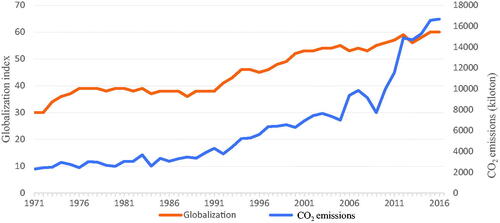
Globalization, which is defined as the integration of world economies (see Scholte 2008) also continues to expand as further depicted in Figure 1. The expansion of globalization has proceeded in different ways including by means of technology transfer, foreign aid, commerce, and intercontinental movement as investments continue to grow across the world. Ghana, which has been generally regarded as one of the quick-growing economies in Africa (Aryeetey et al. 2001; Langnel and Amegavi 2020) is not an exception to this phenomenon. The increasing trend of globalization raises an important issue of public concern among environmental economists and scientists, namely whether globalization contributes negatively or positively to environmental quality. As a result, there have been numerous theoretical and empirical studies to probe the repercussions of globalization on environmental deterioration in emerging economies but to date no consensus has emerged. The relationship between globalization and environmental degradation can be either positive or negative subject to the direction of the shock (Rafindadi and Usman 2019). Yanikkaya (2003) argues that globalization through the lens of trade can lead to the transfer of technological innovation which tends to promote efficient energy use to reduce emissions. He further contends that globalization opens doors for international negotiation to implement environmentally friendly policies to reduce degradation. Questions pertaining to whether these initiatives are effective or not continue to linger and has therefore given rise to an active policy discourse. By contrast, Ahmed et al. (2016) report that globalization, when unchecked, induces natural resource depletion (such as deforestation) and inefficient energy use (such as reliance on petroleum products) which result in an increase of GHG releases. For instance, Shahbaz et al. (2017) describe an inverse relationship between globalization and CO₂ releases in the case of China. In South Africa, however, Rafindadi and Usman (2019) reveal a positive connection between globalization and ecological decay. This notwithstanding, Salahuddin et al. (2019) did not find any significant connection between globalization, urbanization, and CO₂ emissions for 44 African countries.

In the context of developing nations, no consensus has emerged with regard to the relationship between globalization and CO₂ emissions (Rafindadi and Usman 2019). In general, most studies in Ghana assume a linear relationship between globalization, energy use, economic expansion, and ecological decay, without considering the fluctuations in the economy that are likely to affect policies aimed at improving environmental quality (see Aboagye 2017; Twerefou, Danso-Mensah, and Bokpin 2017; Kwakwa and Alhassan 2018). For example, Ghana experienced some economic challenges (such as high inflation, high government debt, and drastic decline in GDP) during the 1980s which continued through the early 2000s (Huq and Tribe 2018). Furthermore, the 2012–2016 energy crises and the global financial crises of 2008 (see Younger 2016) affected most economies and Ghana was no exception. In addition, the country has expanded its trade to countries on other continents by amending various trade policies and has joined international agreements such as the Kyoto Protocol (in 2003) and REDD+ (Reducing Emissions from Deforestation and Forest Degradation) (in 2008) aimed at mitigating GHG emissions and promoting a pollution-free environment (see Asare 2015). It is, therefore, important to incorporate some of these globalization issues and economic recessions when analyzing time-series variables to provide a robust estimation that depicts the dynamics in the economy.

Another limitation of previous studies has to do with measurement of the globalization variable. For instance, in the Ghanaian context, past studies have used variables such as trade openness and urbanization as proxies for globalization (see Sarkodie and Strezov 2019; Abokyi et al. 2021). However, globalization goes beyond urbanization and trade, and for that matter, using these variables might not be sufficiently inclusive to facilitate policy adoption and implementation. As a result, there is the need for studies to incorporate broader measures of globalization and the present study seeks to fulfill this objective for comprehensive policy purposes. Globalization comprises political globalization (membership in international organizations and participation in international agreements), social globalization (remittances, cross-country tourism, and migration), and economic globalization (trade, foreign aid, external income payments, foreign direct investments, and income from international trade). It is reported that, social globalization promotes interaction among countries which promotes tourism and risk of disease infection. Political globalization by contrast enables countries to open up to international treaties and hence to emulate eco-friendly and ecological change policies (see Hironaka 2002; Ahmed et al. 2016). Considerable attention has only been given to the monetary benefits or costs of globalization with virtually no consideration for its social and political dimensions and ecological ramifications (Bilgili et al. 2020). Potrafke (2015) recommends exploring the effects of internationalization which is an aspect of globalization on any phenomenon and the factors that account for a mixed proportion of globalization should be taken into consideration. Regarding the energy-pollution nexus, a plethora of studies has been conducted on the Environmental Kuznets Curve (EKC). In sum, it has been documented that energy use and economic growth contribute positively to environmental degradation (see Kwakwa, Arku, and Aboagye 2014; Asumadu-Sarkodie and Owusu 2016; Katircioğlu and Katircioğlu 2018; Abokyi et al. 2019; Sarkodie and Strezov 2019).

In view of what has been expounded above, the present study contributes to the literature by using Markov-switching (MS) models to investigate the EKC in the context of Ghana for different regimes over the period 1971–2016. This research employs MS models due to their flexibility and ability to detect any possible nonlinear relationship between CO₂ and its determinants. Also, this study investigates the impact of overall and disaggregated indexes of globalization (political, social, and economic) on ecological decay in Ghana. We further employ the Neural Network Autoregression (NNAR [p, k]) machine-learning approach to forecast CO₂ emissions for the country over the next decade. More importantly, this study is the maiden effort to combine MS and the NNAR [p, k] approach to investigate environmental degradation in Ghana.

The remainder of this article proceeds as follows. The next section presents a theoretical and empirical review and this is followed by a discussion of our methodology. We then present the empirical results and provide a discussion of their implications. Finally, we conclude with consideration of this work for policy dialogue as well as highlight limitations and directions for future research.

Literature review

Theoretical conjectures of globalization, energy utilization, economic expansion, and ecological decay

The effect of globalization on the environment can be explained through three channels (Rafindadi and Usman 2019). The first channel is the scale effect which indicates that industrialization triggers economic development and the use of dirty energy such as fossil fuels, specifically, gasoline and diesel. For instance, Ahove and Bankole (2018) indicated that the combustion of fossil fuels and industrial activities induces global warming and ozone-layer depletion by contributing to the emission of CO₂ as well as nitrous oxide (N₂O), sulfur dioxide (SO₂), and nitrogen oxides (NO_x).

The second channel focuses on the make-up effect which suggests that globalization leads to an improvement in carbon-neutral commodities (Langnel and Amegavi 2020). Environmental degradation declines as the economy expands due to an increase in the use of carbon-neutral inputs (see Stern 2007).

The final channel, the technique effect, indicates that globalization promotes innovation, technical know-how, and technology transfers which increase economic growth without impeding the environment (see Dollar and Kraay 2004; Yanikkaya 2003).

Similarly, there are three strands of literature with regard to energy use, economic growth, and the environmental deterioration nexus (see Pao and Tsai 2011). The first strand suggests that energy use and production complement each other, especially in developing countries where production demands high energy use (Belloumi 2009). The second strand examines the relationship between economic growth and energy utilization in the context of the EKC hypothesis—which indicates that there exists an inverted U-shaped relationship between economic growth and environmental degradation. Ecological depletion (or environmental degradation) increases as the economy expands, but declines (indicating improvement in the environmental quality) afterwards (Grossman and Krueger 1991). The final strand of literature argues that environmental pollution continuously increases with economic growth as reported by Ang (2007).

Brief empirical review

Empirical studies of the relationship between globalization and ecological decay have provided divergent outcomes. For instance, Antweiler, Copeland, and Taylor (2001) investigated how the transfer of goods among countries affect the environment and revealed that environmental conditions improve as trade increases. In a related study, Dedeoğlu and Kaya (2013) described a positive relationship between globalization and environmental degradation for 25 member countries of the Organization for Economic Co-operation and Development (OECD). Also, Rafindadi (2016) supported the claim that trade makes environmental conditions better in Nigeria. Similarly, using the generalized method of moments, Twerefou, Danso-Mensah, and Bokpin (2017) concluded that globalization has done more harm than good for 36 sub-Saharan African countries and Shahbaz et al. (2018) confirmed this conclusion for 25 advanced nations in Western Europe, Asia, Oceania, and North America utilizing panel data for the period 1970–2014. Furthermore, Destek, Ulucak, and Dogan (2018) used a second-generation panel-data analysis over the period 1980–2013 and established that clean energy use and trade openness enhance environment conditions in European Union (EU) countries. Salahuddin et al. (2019) also employed a panel-regression methodology and established no significant relationship between globalization and CO₂ emissions for 44 African countries.

By contrast, urbanization increases environmental pollution. In Italy, Saint Akadiri et al. (2019) employed the autoregressive distributed lag (ARDL) model to explore the nexus between output, globalization, and overall energy consumption (such as electricity, natural gas, geothermal heat, solar energy, and biomass waste). The study found a positive relationship between globalization and CO₂ emissions. Destek (2020) employed a panel data-estimation technique to investigate the influence of an overall and disaggregated globalization index on CO₂ releases in several Central and Eastern European countries from 1995 to 2015. The author indicated that while economic, social, and overall processes of globalization promote environmental degradation, political globalization improves environmental quality. In a related study on Ghana, Langnel and Amegavi (2020) also report that economic and social globalization do not have a positive effect on the environment. The authors, however, indicate that political globalization facilitates environment improvement through reduction in CO₂ emissions. Similarly, Rahman (2020) reported that trade makes environmental conditions better for the United States, the UK, Brazil, and China.

In the years following formulation of the EKC theory (see Grossman and Krueger 1991), there were several investigations across the globe to either verify, contest, or establish a countervailing theory with respect to how energy use and economic growth effect the environment. According to Rafindadi and Usman (2019), these several investigations were due to accelerated changes in the distribution of chemical elements (such as CO₂, N₂O, and SO₂) that pose a threat to humans and the environment. Consequently, there have been opposing views on this phenomenon. For instance, Mukhopadhyay and Chakraborty (2005) revealed that the EKC proposition does not hold for the case of India. Similarly, Omisakin and Olusegun (2009) also found no support for the notion of an EKC for Nigeria but in a related study Shahbaz et al. (2013) employed the vector error correction (VECM) estimation technique to confirm the existence of an EKC for Turkey during the period 1970–2010. The authors further showed that economic diversification accelerates CO₂ emissions. Furthermore, Rafindadi (2016) investigated the EKC hypothesis in Nigeria for the period 1971–2011 using innovation-accounting methods and the author reported that economic expansion initially undermined environmental quality but resulted in subsequent improvement, thus confirming the EKC. Using data from the period 1960 to 2013 and applying the ARDL technique, Ozatac, Gokmenoglu, and Taspinar (2017) also confirmed the existence of the EKC for Turkey. By contrast, Katircioğlu and Ktircioğlu (2018) argued that although fossil fuels harm the environment, the EKC does not exist for the case of Turkey.

Specifically with respect to Ghana, Kwakwa, Arku, and Aboagye (2014) explored the nexus among environmental degradation, agriculture, and industrial growth in the country within the error correction model (ECM) framework and found evidence to support an EKC. Evidence from Twerefou, Bekoe, and Adusah-Poku (2016) showed that as the economy expands, the environment improves at the initial stage and deteriorates afterwards, indicating the absence of an EKC for Ghana. By contrast, Aboagye (2017) and Kwakwa and Alhassan (2018) confirmed the existence of the EKC for the country in the long run. The detrimental impact of energy use on environmental quality was also confirmed by Kwakwa (2019) for Ghana. Similarly, Abokyi et al. (2019) use the ARDL framework and the Bayer-Hanck approach to cointegration and establish a U-shaped relationship between industrial development and CO₂ releases. Furthermore, the authors concluded that fossil-fuel consumption harms the environment in Ghana. In a related study, Langnel and Amegavi (2020) utilized the ARDL framework to examine the connection between ecological degradation and economic expansion in Ghana. The authors revealed that both unclean energy use and economic expansion contribute to environmental deterioration. The study used time-series data for the period 1970–2010 and applied the ADRL model to the dataset. Recently, Kwakwa (2021) confirmed the existence of the EKC in Ghana. Also, the author found no significant relationship between electricity consumption and CO₂ emissions.

Finally, exploring the nexus between agriculture-factor productivity and environmental degradation for 38 sub-Saharan African countries over the period 1981–2016, Alhassan (2021) reported the absence of impacts suggested by the EKC. This finding supported the recent study by Minlah and Zhang (2021).

CO₂ prediction

Considering the importance of the natural environment, researchers have used different models to forecast the volume of CO₂ releases. For example, machine-learning forecasting methods, specifically artificial neural networks (ANNs), have been used extensively in this regard. For instance, Sharda and Patil (1990) confirmed that ANN prediction performs better than the Box-Jenkins approach because the ANN provides the fewest prediction errors. In an empirical study, Liu et al. (2012) applied a neural network model to predict CO₂ emissions in China from 1990 to 2010. The results showed that the country’s emissions would soon reach a maximum point, after which the emission level would decrease. In Serbia, Radojević et al. (2013) employed the ANN method to forecast CO₂ production over the period 1999–2007. The results demonstrated that the ANN method provides good results with less than 10% error.

Abdullah and Pauzi (2015) reviewed literature on methods of modeling and forecasting CO₂ releases from the period 2003 to 2013. Out of 42 articles, ANN models were revealed to be the most frequently used method, followed by grey models (GM), computer-based methods, T1 and T2 approaches involving use of the method of the Intergovernmental Panel on Climate Change (IPCC), optimal growth approach, and fuel analysis. Linear regression and other methods such as the logistic function and survey-travel information are found be the least frequently used. In a related study, Ayvaz, Kusakci, and Temur (2017) used grey models to forecast CO₂ emissions in Turkey and Appiah et al. (2018) predicted CO₂ emissions in emerging economies using ANN of a two-stratum feed-forward neural network. The authors indicated that ANN provides the fewest prediction errors. In India, Amarpuri et al. (2019) utilized a deep learning hybrid model of the Conventional Neural Network of Long Short-Term Memory (CNN-LSTM) to forecast CO₂ emissions and the results show that CO₂ emissions in India are likely to rise for the next decade.

From the literature highlighted, it is imperative that such predictions and forecasting be carried out for the case of Ghana. This is so because projecting future ecological dynamics in the context of the country would aid policy makers, environmentalists, and scientists in designing eco-friendly programs and strategies to mitigate environmental problems in the economy. Again, this is very important because Ghana aims to achieve a 15% reduction in CO₂ emissions by 2030, and therefore, there is an urgent need for a timely study to guide stakeholders in policy making.

Methodology

This section is devoted to outlining the methodology of the study and specifically focuses on the data, model specification, and estimation techniques.

Data

The study utilizes secondary data for the period 1971–2016. This choice is influenced by the availability of data for the variables used in the study. The variables are CO₂ emissions (which are the releases that emanate from the combusting of fossil fuels and the manufacturing of cement—it includes the carbon emissions produced during the consumption of liquid, solid, and gas fuels) measured in kilotons (kt), an overall globalization index (GI) (and disaggregated globalization indexes (political [PGI], social [SGI], and economic [EGI])), GDP per capita ([Y], measuring economic growth), and energy use per capita (EU). Data on globalization is extracted from the KOF globalization index of the Swiss Economic Institute (see Gygli et al. 2019), the remaining variables are sourced from the World Bank’s World Development Indicators ([WDI], World Bank 2020). Moreover, these variables are chosen based on their connection with the Sustainable Development Goals (SDGs)—specifically, SDG 6, 7, and 13, which are related to achievement of clean energy and a pollution-free environment (see Morton, Pencheon, and Squires 2017). Clean energy and a pollution-free environment could be accelerated by the interplay of globalization through trade and international treaties as well as through the transfer of energy-efficient products and global agreements on environmental conservation. Also, the KOF globalization measure provides a robust proxy for globalization because it accounts for political, social, and economic factors. All the variables are expressed in log values to ensure covariance stationary. Finally, to ensure that the variables are stationary for reliable and efficient results, we use the Augmented Dickey-Fuller (ADF) (Dickey and Fuller 1981), Phillips and Perron (PP) (Phillips and Perron 1988), and Zivot and Andrews (ZA) (Zivot and Andrews 2002) for the unit root tests.

Markov-switching model

Most empirical studies on environmental degradation and globalization have ignored the possibility of a nonlinear association between these two variables as well as other macroeconomic variables. The Ghanaian economy has in recent years gone through a series of political, economic, and structural transformation programs in response to various macroeconomic instabilities. It is, therefore, important to consider these dynamics in time-series modeling to provide a more reliable result for effective policy purposes. This study, therefore, uses the Markov-switching (MS) models to probe these dynamics in the variables. Given the advantages of MS models in time-series frameworks over other techniques, they have been used in many influential studies (see Goodwin 1993; Bilgili et al. 2020).

The MS models are able to account for changes in the structures of the economy that can affect the relationships among the variables under investigation. Also, the estimated coefficients of the models are time-variant and they exclusively depend on the regimes of the variables. That is, the condition of the variables in the current state, t, is solely determined by the state from a period ago (t − 1), which causes the model to switch from one state to another by means of a probabilistic framework. The transition is regulated by an unobserved, ergodic uniform Markov chain (Hamilton 1989). Therefore, the interaction among the variables could be different in each state of the economy. For the purposes of this study, two regimes (two states of the economy) are employed. The basic model is expressed as follows: (1) $$Y_t=\{\begin{array}{c}{\theta }_{1,2}+{\theta }_{1,1}{Z}_t+{\mu }_t|s_t=1\\ {\theta }_{2,1}+{\theta }_{2,2}{Z}_t+{\mu }_t|s_t=2\end{array}$$(1) where, Y_t and Z_t denote a vector of dependent and independent variables respectively, ${\mu }_t$ is the error term assumed to have zero mean and constant variance, ${\mu }_t\sim N(0,{\sigma }_{s_t}^2)$ and $s_t$ denotes the state of the economy. Specifically, the MS models for this study are specified in Equations 2(2) $$MS1:ln{{CO}_2}_t={\alpha }_{0,s_t}+{\alpha }_{1,s_t}ln{Y}_t+{\alpha }_{2,s_t}ln{Y}_t^2+{\eta }_{t1}$$(2) , 3(3) $$MS2:ln{{CO}_2}_t={\beta }_{0,s_t}+{\beta }_{1,s_t}ln{Y}_t+{\beta }_{2,s_t}ln{Y}_t^2+{\beta }_{3,s_t}ln{EU}_t+{\beta }_{4,s_t}ln{GI}_t+{\eta }_{t2}$$(3) and 4(4) $$MS3:ln{{CO}_2}_t={\delta }_{0,s_t}+{\delta }_{1,s_t}ln{Y}_t+{\delta }_{2s_t}{Y}_t^2+{\delta }_{3,s_t}ln{EU}_t+{\delta }_{4,s_t}ln{\mathit{PGI}}_t+{\delta }_{5,s_t}ln{\mathit{SGI}}_t+{\delta }_{6,s_t}ln{\mathit{EGI}}_t+{\eta }_{t3}$$(4) . (2) $$MS1:ln{{CO}_2}_t={\alpha }_{0,s_t}+{\alpha }_{1,s_t}ln{Y}_t+{\alpha }_{2,s_t}ln{Y}_t^2+{\eta }_{t1}$$(2) (3) $$MS2:ln{{CO}_2}_t={\beta }_{0,s_t}+{\beta }_{1,s_t}ln{Y}_t+{\beta }_{2,s_t}ln{Y}_t^2+{\beta }_{3,s_t}ln{EU}_t+{\beta }_{4,s_t}ln{GI}_t+{\eta }_{t2}$$(3) (4) $$MS3:ln{{CO}_2}_t={\delta }_{0,s_t}+{\delta }_{1,s_t}ln{Y}_t+{\delta }_{2s_t}{Y}_t^2+{\delta }_{3,s_t}ln{EU}_t+{\delta }_{4,s_t}ln{\mathit{PGI}}_t+{\delta }_{5,s_t}ln{\mathit{SGI}}_t+{\delta }_{6,s_t}ln{\mathit{EGI}}_t+{\eta }_{t3}$$(4) where, CO₂ is carbon dioxide (a proxy for ecological decay), EU represents per capita energy consumption, GI is an overall globalization index, and Y denotes output per capita. PGI, SGI, and EGI are political, social, and economic globalization indexes, respectively. The error terms are${ \eta }_{ti},$ where i = 1, 2, 3. Following (Shahbaz et al. 2015), Equation 2(2) $$MS1:ln{{CO}_2}_t={\alpha }_{0,s_t}+{\alpha }_{1,s_t}ln{Y}_t+{\alpha }_{2,s_t}ln{Y}_t^2+{\eta }_{t1}$$(2) is estimated to investigate the conventional EKC theory in the Ghanaian context. Equation 3(3) $$MS2:ln{{CO}_2}_t={\beta }_{0,s_t}+{\beta }_{1,s_t}ln{Y}_t+{\beta }_{2,s_t}ln{Y}_t^2+{\beta }_{3,s_t}ln{EU}_t+{\beta }_{4,s_t}ln{GI}_t+{\eta }_{t2}$$(3) analyzes the EKC theory, the impact of an overall globalization measure, and energy utilization on CO₂ emissions (see Rafindadi and Usman 2019). Finally, Equation 4(4) $$MS3:ln{{CO}_2}_t={\delta }_{0,s_t}+{\delta }_{1,s_t}ln{Y}_t+{\delta }_{2s_t}{Y}_t^2+{\delta }_{3,s_t}ln{EU}_t+{\delta }_{4,s_t}ln{\mathit{PGI}}_t+{\delta }_{5,s_t}ln{\mathit{SGI}}_t+{\delta }_{6,s_t}ln{\mathit{EGI}}_t+{\eta }_{t3}$$(4) investigates the EKC theory, as well as the effect of energy use and the disaggregated globalization measures on CO₂ emissions.

The likelihood that the system switches to a different regime or stays in the same regime is expressed in Equation 5(5) $$\mathrm{Pr}\left({\mathit{regime}}_t=1|{\mathit{regime}}_{t-1}=2\right)=p_{21}=1-p_{22}$$(5) . $$\mathrm{Pr}\left({\mathit{regime}}_t=1|{\mathit{regime}}_{t-1}=1\right)=p_{11}$$ $$\mathrm{Pr}\left({\mathit{regime}}_t=2|{\mathit{regime}}_{t-1}=1\right)=p_{12}=1-p_{11}$$ (5) $$\mathrm{Pr}\left({\mathit{regime}}_t=1|{\mathit{regime}}_{t-1}=2\right)=p_{21}=1-p_{22}$$(5) $$\mathrm{Pr}\left({\mathit{regime}}_t=2|{\mathit{regime}}_{t-1}=2\right)=p_{22}$$ where $p_{12}$ and $p_{21}$are the likelihood that the system changes from state 1 to state 2 and from state 2 to state 1 respectively, $p_{11}$ and $p_{22}$ are the probabilities that the system stays in state 1 or state 2, and Pr denotes probability. The system would be in continuous transformation if $p_{21}=p_{12}=1$ and $p_{11}=p_{22}=0.$ By contrast, the system remains static if $p_{21}=p_{12}=0$ and $p_{11}=p_{22}=1.$ The probability lies between 0 and 1 ($0\le p_{ij}\le 1$) and they sum up to unity. The parameters are all contingent on the state of the economy because its current state is influenced by its previous state.

Neural network antirecession

The Artificial Neural Network (ANN) prediction approach is fundamentally motivated by how the human brain functions. This approach allows for a network of nonlinear connection between the affected variable and its determinants. It is a system that is organized in stratum. The predictor variable (input) forms the layer below while the variable to be predicted (output) constitutes the topmost stratum; there may be layers in between (hidden neutrons). The fundamental formulation of the model is similar to a linear regression model. However, when an intermediate stratum is added, the model then takes the form of a nonlinear function (Figure 2).

Figure 2. Multilayer-feed-forward system of 4 inputs. Source: Adopted from As’ad, Sujito, and Setyowibowo (2020).

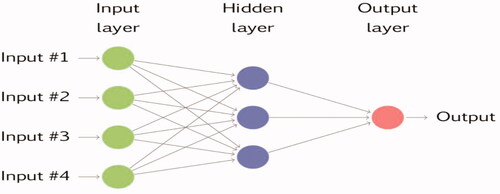
The output of an intersection in a stratum serves as the input for the next. The inputs of one intersection, j, are linearly combined using weights. Afterwards, the result is then nonlinearly transformed to give a required output of the next stratum. The linear combination and the nonlinear modification are specified in Equations 6(6) $$y_j=a_j+\sum _{i=1}^k{x}_{i,j}{z}_i$$(6) and 7(7) $$s\left(y\right)=\frac{1}{1+e^{-y}}$$(7) . (6) $$y_j=a_j+\sum _{i=1}^k{x}_{i,j}{z}_i$$(6) (7) $$s\left(y\right)=\frac{1}{1+e^{-y}}$$(7) where $y_j$ is the function of j hidden stratum, $a_j$ denotes weight in the bias unit to j, $x_{i,j}$ represents weight of stratum i, and $z_i$ denotes input network.

Similar to the linear autoregressive time-series models (such as ARIMA), lagged values can be employed as an input in a neural framework. This is referred to as Neural Network Autoregression, NNAR(p,k), where p is the optimal number of lags and k denotes the number of hidden strata. For instance, NNAR(4, 3) means that the previous 4 observations of the series are employed as an input (p = 4) and 3 hidden strata (k = 3) are utilized to predict a given output, $x_t.$ For the purpose of prediction, the network is trained repetitively through at least 20 iterations and the output is the average of the estimations. This study uses the nnet() package in R software for estimation of the model.

Following As’ad, Sujito, and Setyowibowo (2020), the first procedure in forecasting is to examine the properties of the series to know whether they exhibit seasonal, random walk, or trending behavior. If the data portrays strong seasonal dynamics, then a seasonal element, P, is introduced in the NNAR model (NNAR[p,P,k]); otherwise, it is considered as zero. Thereafter, the autoregressive (ACF) and the partial autoregressive functions (PACF) are used to determine the a priori maximum lag orders to formulate the model. The seemingly best model is selected contingent on the smallest value of the root mean squared error (RMSE) and mean absolute percentage error (MAPE) of the training and testing values. The RMSE and the MAPE are specified in Equations 8(8) $${\mathit{RMSE}}_h=\sqrt{\frac{\sum _{t=1}^T{\left(e_{t+h}\right)}^2}{N}}$$(8) and 9(9) $${\mathit{MAPE}}_h=\frac{1}{n}\sum _{t=1}^n|\frac{e_{t+h}}{z_t}|$$(9) . (8) $${\mathit{RMSE}}_h=\sqrt{\frac{\sum _{t=1}^T{\left(e_{t+h}\right)}^2}{N}}$$(8) (9) $${\mathit{MAPE}}_h=\frac{1}{n}\sum _{t=1}^n|\frac{e_{t+h}}{z_t}|$$(9) where, N, n, e, h and ${\mathrm{z}}_{\mathrm{t}}$ represent sample size, number of iterations, forecast bias, forecast horizon, and actual value of the series.

Results

This section presents the results and provides a discussion of the study. Specifically, it focuses on the descriptive statistics of the variables used, unit root test, and the empirical results.

Descriptive statistics

A summary of the descriptive statistics of the variables is reported in Table 1. It is observed that energy use, overall globalization, political globalization, and economic globalization are negatively skewed while CO₂, economic growth, and social globalization are positively skewed. The Jarque-Bera test indicates that all the variables—per capita income (Y), CO₂, energy use (EU), overall globalization (GI), economic globalization (EGI), political globalization (PGI), and social globalization (SGI) are normally distributed. The standard deviation values also show that the data do not deviate much from their respective mean values. The time-series plot of the variables (see Figure A.1 in the Appendix) show that, at first difference, all the variables exhibit a random walk.

Table 1. Summary statistics.

	lnCO2	lnY	lnEU	lnGI	lnPGI	lnSGI	lnEGI
Mean	8.546	6.196	5.823	3.795	4.226	3.070	3.635
Median	8.477	5.933	5.840	3.784	4.251	2.970	3.653
Maximum	9.721	7.760	6.012	4.094	4.397	3.763	3.941
Minimum	7.739	5.433	5.584	3.401	3.722	2.804	3.329
Std. Dev.	0.601	0.652	0.111	0.195	0.156	0.284	0.192
Skewness	0.448	1.175	−0.617	−0.046	−1.394	1.380	−0.008
Kurtosis	2.024	2.942	2.493	1.813	5.319	3.593	1.593
Jarque-Bera	3.365	10.600	3.436	2.718	25.213	15.279	3.797
Probability	0.186	0.225	0.179	0.257	0.061	0.120	0.150
Sum	393.125	284.998	267.880	174.565	194.415	141.211	167.195
Sum Sq. Dev.	16.239	19.146	0.556	1.716	1.095	3.636	1.651
Observations	46	46	46	46	46	46	46

Unit root test results

Most time-series data exhibit seasonal trends, and therefore may contain a unit root. A shock to a nonstationary series will have a permanent impact on the future values, and for that matter the variance, mean, and covariance will be time-dependent (Gujarati 2003). Consequently, econometric analysis involving nonstationary variables may produce spurious results (Tang and Tan 2013). Therefore, stationarity tests are conducted to ascertain the series properties of the variables. This is also to ensure that none of the series is stationary at the second order, I(2). The test results are reported in Table 2.

Table 2. ADF and P − P stationarity test results.

ADF test					PP test
Variable	Constant	Order of Int.	Constant and trend	Order of Int.	Constant	Order of Int.	Constant and trend	Order of Int.
Level
lnCO2	2.01		−3.01		1.34		−2.78
lnY	0.26		−1.15		0.26		−1.24
lnEU	−1.66		−2.06		−1.85		−2.28
lnGI	−1.37		−2.27		−1.36		−2.49
lnPGI	−4.04***	I (0)	−4.32***	I (0)	−4.18***	I (0)	−4.48***	I (0)
lnSGI	−1.24		−1.03		1.11		−0.97
lnEGI	−1.65		−3.12		−1.52		−2.51
First-difference
lnCO2	−5.99***	I (1)	−6.81***	I (1)	−12.28***	I (1)	−22.95***	I (1)
lnY	−5.94***	I (1)	−5.97***	I (1)	−5.94***	I (1)	−5.98***	I (1)
lnEU	−6.18***	I (1)	−6.10***	I (1)	−6.17***	I (1)	−6.10***	I (1)
lnGI	−6.55***	I (1)	−6.57***	I (1)	−6.59***	I (1)	−6.62***	I (1)
lnPGI	−5.51***	I (1)	−6.16***	I (1)	−5.59***	I (1)	−6.24***	I (1)
lnSGI	−5.31***	I (1)	−3.77**	I (1)	−5.33***	I (1)	−6.19***	I (1)
lnEGI	−7.31***	I (1)	7.22***	I (1)	−7.48***	I (1)	−7.38***	I (1)

Note. *** and ** represent 1%, and 5% level of importance respectively. The appropriate lag (s) is automatically chosen by the AIC for the ADF test and Newey-West Bandwidth accordingly. The optimal lag for the ADF and P − P tests are 1 and 3, respectively.

From Table 2, it is observed that except for political globalization which is stationary at level, I(0), the remaining variables are stationary at the first difference, I(1). Since the ADF and the PP test do not explicitly account for structural break(s) in the unit root test, the Zivot- Anderws (ZA) unit root test is employed for a robustness check. The outcome of the ZA unit root test (see Table A1 in the Appendix) indicates the same order of integration as revealed by the ADF and PP tests.

Markov-switching models

The results from the two regimes Markov-switching models are reported in Table 3.

Table 3. Markov-switching models results.

	MS1 model		MS2 model		MS3 model
Variable	Regime 1	Regime 2	Regime 1	Regime 2	Regime 1	Regime 2
Constant	17.504***	7.549**	−1.111	18.297***	−15.894***	−9.802***
lnY	−3.033***	−0.580	0.471	−3.833***	−0.539	−0.913***
lnY2	0.263***	0.113	−0.059	0.340***	0.144	0.147***
lnGI			2.212***	0.899**
lnEU			0.335**	−0.478	0.561***	−0.412***
lnPGI					5.325***	−0.806***
lnSGI					0.588**	−0.938***
lnEGI					−0.452	2.019***

Note. *** and ** denote the significance levels at 1% and 5% respectively; MS1 model considers the traditional EKC theory without any control variable; MS2 model investigates the EKC theory, while controlling for an overall globalization and energy use; MS3 model focuses on the EKC theory as well as the effect of the three disaggregated globalization variables—political, social, and economic.

From Table 3, the three MS models reveal the nonexistence of an EKC for Ghana; the study reveals a U-shaped as opposed to the traditional inverted U-shape proposed by Grossman and Krueger (1991). Specifically, the U-shaped EKC is observed in MS1 (Regime 1), MS2 (Regime 2), and MS3 (Regime 2). It is also revealed that overall globalization (in both regimes) and energy use (in Regime 1) cause more harm to the environment (see MS2 Model). This finding supports the assertion by Cole (2006) that globalization promotes economic activities through the scale effect which in turn triggers the use of unclean fuel sources and thus reduces the quality of the environment. This outcome is consistent with the findings by Twerefou, Danso-Mensah, and Bokpin (2017) for 36 sub-Saharan African countries and Shahbaz et al. (2018) for 25 advanced nations in Western Europe, Asia, Oceania, and North America. However, Rafindadi and Usman (2019) report otherwise for South Africa.

The nonexistence of EKC in the country means that as the economy expands, CO₂ emissions initially reduce to a certain point and increase thereafter. Therefore, CO₂ emissions increase as economic growth increases. The non-confirmation of the EKC theory in the present study may be attributed to the fact that as per capita GDP increases, Ghana is not able to consume environmentally-friendly products that are likely to reduce CO₂ emissions. Another reason could be that as the economy expands, Ghana is not able to diversify its energy portfolio to incorporate clean energy sources that have the tendency to reduce CO₂ emissions, hence the income effect may not be sufficient to promote environmental quality. This result is consistent with Twerefou, Bekoe, and Adusah-Poku (2016), Abokyi et al. (2019), and Minlah and Zhang (2021) for the case of Ghana and Mukhopadhyay and Chakraborty (2005) for India. However, it contradicts those of Kwakwa, Arku, and Aboagye (2014, Kwakwa 2021), Aboagye (2017), and Kwakwa and Alhassan (2018) who report the existence of an EKC for Ghana. The difference in outcome is plausible because, for instance, Kwakwa, Arku, and Aboagye (2014) focused only on agricultural and industrial growth while the present study uses per capita GDP which comprises all of the sectors of the economy. Moreover, data for the present study are an extension of those used by Aboagye (2017) and Kwakwa and Alhassan (2018). Finally, the present study uses a non-linear model that is able to capture the dynamics in different regimes as compared to the linear models used by the above-mentioned studies which may not be able to capture the dynamics and shocks in the data at different regimes of the economy.

The results from the MS3 model also indicate that political globalization and social globalization improve environmental quality in Regime 2 but harm the environment in Regime 1. This shows the dynamic effects of political and social factors on the environment. Finally, economic globalization is revealed to cause deterioration of the environment in Regime 2 through the CO₂ emissions.

The results from the MS3 model imply that economic globalization tends to increase CO₂ emissions through trade in goods and services, foreign direct and portfolio investments, and income payments. Economic globalization induces economic activities through trade and investment which may cause a rise in fossil-fuel consumption and, consequently, undermine the quality of the environment. Again, political and social globalization are revealed to have diverse effects on the environment in different regimes. While political globalization (comprising multinational corporations and treaties, embassies, and international organizations) and social globalization (comprising international students and tourism, migration, and foreign transfers) are found to have a negative influence on the environment through CO₂ emissions in Regime 1, they tend to reduce CO₂ emissions in Regime 2 and, hence, improve environmental quality. A study by Destek (2020) finds similar results for Central and Eastern European countries.

Furthermore, to ascertain the likelihood of transition from one period to another or staying in the same period, we estimated the transition probabilities and the results are reported in Table 4. It is observed that $P_{11}$ and $P_{22}$ exhibit high probability values (above 90% in MS1 and MS2 Models) which suggest that the MS1 and MS2 Models would remain in the same regime. Therefore, it is less than 10% likely that MS1 and MS2 would switch between regimes. For instance, it is 1.8% and 5.1% probable that the MS1 Model would change from Regime 1 to Regime 2 and from Regime 2 to Regime 1, respectively (see Figures 3 and 4). By contrast, the MS3 Model shows an irregular transition probability. Specifically, it is 84.3% ($P_{11}$) and 71% ($P_{22}$) probable that the model would stay in Regime 1 and Regime 2, respectively, and it is 29% ($P_{12}$) and 15.7% ($P_{21}$) probable that the model would shift from the first regime to the second regime.

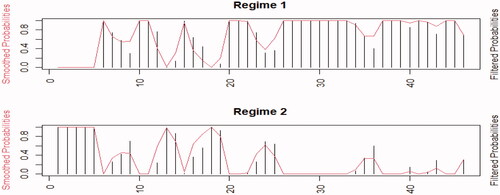
Figure 3. Smoothed probablity for MS1 Model.

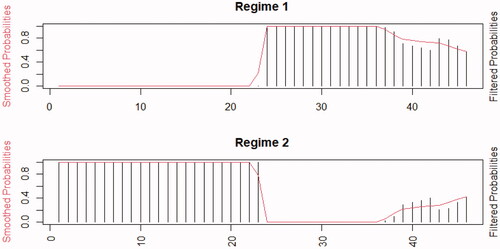
Figure 4. Smoothed probability for MS2 Model.

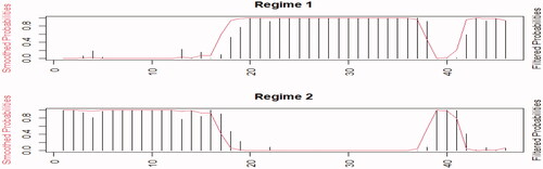
Table 4. Transition probabilities and model specification test results.

Transition probability	MS1 model	MS2 model	MS3 model
$P_{11}$	0.949	0.942	0.843
$P_{12}$	0.018	0.058	0.290
$P_{22}$	0.998	0.942	0.710
$P_{21}$	0.051	0.079	0.157
Diagnostic test
Model specification test [p-values]	0.507	0.974	0.642

Note. $P_{11}$ and $P_{22}$ represent the likelihood that the model stays in regime 1 and regime 2 respectively. $P_{12}$ and $P_{21}$ denote the likelihood that the model transitions from regime 1 to regime 2 and from regime 2 to regime 1 respectively.

It is further observed from Table 4 that the null hypothesis of model misspecification is rejected at the 5% significance level. Therefore, we can conclude that the nonlinear model used for the estimation of the MS models is correctly specified.

Another advantage of the MS models is that they generate the duration of the regimes and the periods they cover. Figure 3 shows the smooth probability graph of the regimes based on the MS1 Model. The first regime covers the period 1994–2016 while the second regime covers 1971–1993, indicating that each regime spans 23 years.

Figure 4 depicts the smooth probability graph based on the MS2 Model. Regime 1 covers the periods of 1987–2007 and 2012–2016 while the second regime covers the periods of 1971–1986 and 2008–2011.

Figure 5 (transition probability based on the MS3 Model), by contrast, depicts irregular transition probabilities. This probably shows the dynamic in the economic, social, and political environment and how they affect ecological decay. Regime 1 covers the period of 1976–1982 and 1990-2016 while Regime 2 covers 1971–1975 and 1983–1989.

Figure 5. Smoothed probability for MS3 Model.

Residual diagnostics

Based on the MS models (1, 2, and 3), we plotted the residuals of the series to check normality and serial correlation issues of the data. The plots are shown in Figures 6–8.

Figure 6. Q–Q, ACF, and PACF plots from MS1 Model.

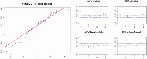
Figure 7. Q–Q, ACF, and PACF plots from MS2 Model.

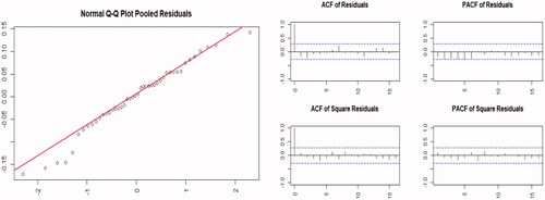
Figure 8. Q–Q, ACF, and PACF plots from MS3 Model.

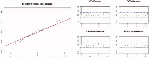
The quantile-quantile (Q–Q), the autocorrelation function (ACF), and the partial autocorrelation function (PACF) tests show that, generally, the time-series data follows the Gaussian distribution and, therefore, the residuals are normally distributed. Specifically, the majority of the data points are either on or closely around the Q-Q normality line. This means that the estimated coefficients in the MS models are reliable and robust.

Neural network autoregression (NNAR) forecasting

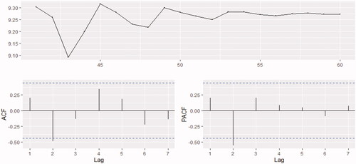
The ACF and PACF are utilized to provide preliminary intuition of the proposed maximum past values to be used for the NNAR model. Figure 9 shows that the maximum past values are 13 and there is no seasonality in the data. In this case, the stratum, k = 7 [(13 + 1)/2] and the seasonal element, $P=0.$ Therefore, the suggested provisional model for predicting environmental degradation is NNAR(13, 7). We also tested other models such as NNAR(11, 6), NNAR(12, 6), NNAR(14, 8), and NNAR(15, 8) (see Table 5). The prediction horizon is from 2011 to 2030 (h = 20). The relatively better model is selected based on the smallest RMSE and MAPE error values of the model training.

Figure 9. Series plot, ACF, and PACF of ${\mathit{CO}}_2$ emisions in Ghana.

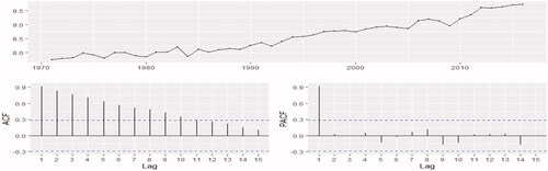
Table 5. Measures of accuracy of the NNAR(p, k) trainning models.

Model	Weight	RMSE	MAPE
NNAR(11, 6)	79	0.00131	0.00980
NNAR(12, 6)	85	0.00164	0.00855
NNAR(13, 7)	106	0.00033	0.00283
NNAR(14, 8)	129	0.00020	0.00175
NNAR(15, 8)	137	0.00041	0.00320

The results from Table 5 show that model NNAR(14, 8) recorded the least RMSE and MAPE and this is followed by model NNAR(13, 7) and model NNAR(15, 8) in that order. For the purpose of this study, NNAR(14, 8) is utilized for the pridiction.

The model is iterated at least 20 times and the average value of the total output is used for the forecasting and the input is linearly weighted. Figure 10 shows the prediction horizon of 20 years. The forecast is shown by the blue line. It can be observed that CO₂ emissions in Ghana from 2011 to 2030 depict an upward trend. There is, therefore, the likelihood that the environment, if not well managed, would continue to deteriorate in terms of CO₂ emissions for the next decade. The study proceeds to estimate the forecast values against the available actual values based on the NNAR(14, 8) model and the results are reported in Table 6.

Figure 10. NNAR(14, 8) prediction (Annual ${CO}_2$ growth in Ghana, 2011–2030).

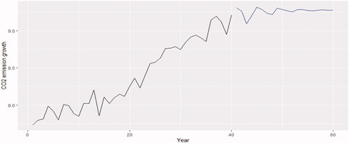
Table 6. Predicted values of the NNAR(14, 8) model.

Year	NNAR(14, 8) forecast	Actual	Difference
2011	9.3033	9.3523	0.0490
2012	9.2596	9.6066	0.3470
2013	9.0913	9.5944	0.5032
2014	9.2011	9.6334	0.4323
2015	9.3166	9.7143	0.3977
2016	9.2814	9.7214	0.4396
2017	9.2318	9.6894	0.4576
2018	9.2174	9.6949	0.4776
2019	9.3011	9.7313	0.4302
2020	9.2814
2021	9.2654
2022	9.2504
2023	9.2830
2024	9.2824
2025	9.2715
2026	9.2659
2027	9.2740
2028	9.2780
2029	9.2731
2030	9.2724

The maximum prediction difference is 0.5032 which occurred in 2013. On average, the model (NNAR[14, 8]) performs well (see Figure 11) in predicting CO₂ emissions for Ghana with average RMSE and MAPE of 0.26051 and 0.02295, respectively. This prediction indicates that environmental quality in Ghana is likely to deteriorate in the next decade. This is in line with Twerefou, Bekoe, and Adusah-Poku (2016) and EPA (2015) assertions that Ghana has circumvented the minimum turning point of the U-shape relationship of its environmental-growth nexus since the late 1990s and early 2000s. This implies that CO₂ emissions may continue to rise in the future (as shown by the results in Table 3) if immediate mitigation measures are not taken.

Figure 11. Predicted NNAR(14, 8) values.

Conclusions and policy implications

This study examined the EKC in the context of Ghana using CO₂ emissions, energy utilization, and KOF globalization indexes. We investigated which of the KOF globalization indexes is the major driver of CO₂ emissions. To do so, we utilized secondary time-series data spanning the period 1971–2016 and employed Markov-switching models for the analysis. Subsequently, the Neural Network autoregression (NNAR[p,k]) machine-learning approach was adopted to forecast CO₂ emissions from 2020–2030.

The results from all three of the esteimated MS models confirm the nonexistence of an EKC for Ghana. The study specifically revealed a U-shaped EKC which is contrary to the conventional inverted U-shaped curve. The U-shaped EKC is observed in MS1 Model (Regime 1), MS2 Model (Regime 2), and MS3 Model (Regime 2). With regard to the other variables used in the study, we conclude that, in general, overall globalization and energy utilization harm the environment. Based on the results from the disaggregated globalization analysis, the study concludes that economic globalization results in deterioration of environmental quality by promoting CO₂ emssions. Political and social globalization, by contrast, have different effects on the environemnt in different regimes—they harm the environment in Regime 1 and improve it in Regime 2. Finally, based on the NNAR(14, 8) forecasted results, we conclude that Ghana will have an upward trend of CO₂ emissions between 2020–2030.

The findings of this study have vital policy implications for Ghana and other countries that share similar characteristics. Following the U-shaped EKC reveals that there is an urgent need to strengthen and/or revise environmental policies in Ghana to protect the environment in expectation of the continuous growth in globalization. Specifically, the Environmental Protection Agency (EPA) Act 490 and Chapter Six, Article 41 (k) of the 1992 constitution which are devoted to protecting and safeguarding the environment should be enforced and/or revised to incoporrate mitigation strategies that are in line with the Paris Agreement and Kyoto Protocol. These measures are likely to curb the increase of GHG emissions as the economy expands. Again, there is the need for the country to invest in clean (renewable) energy technologies. It is also important to promote industrial and domestic energy efficiency through globalization—by importing energy-efficient inputs and consumer goods, such as household appliances. Last but not least, Ghana needs to strengthen its international initiatives such as reducing emissions from deforestation and forest degradation (REDD+) in order to achieve its aim of reducing CO₂ emmissions by 15% by 2030.

This study, however, is not free from limitations. The work reported here could not be extended to the current period due to data unavailability. Also, our research uses only CO₂ emissions as a measure of environmental degradation. Therefore, future studies should consider other forms of environmental quality/degradation such as the ecological footprint.

Disclosure statement

The authors declare that they have no known competing interest or personal relationship that could have influenced the work reported in this paper.

Appendix A

 

Figure A1. Time-series plots of the variables used in the study (level and first difference).

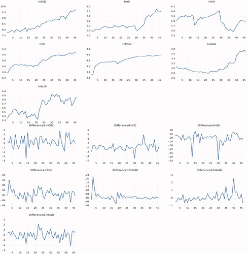
Table A1. Zivot-Andrews (ZA) stationarity test results.

Variable	Constant	Order of It.	Constant and trend	Order of Int.	Break points
Level
lnCO2	−4.57		−5.37		1983
lnY	−4.76		−4.04		2005
lnEU	−4.72		−4.65		1999
lnGI	−3.25		−4.12		1992
lnPGI	−9.33***	I (0)	−9.33***	I (0)	1972
lnSGI	−3.08		−3.23		2009
lnEGI	−4.78		−5.08		1991
First difference
lnCO2	−9.46***	I (1)	−9.68***	I (1)	2008
lnY	−7.32***	I (1)	−7.46***	I (1)	2000
lnEU	−6.72***	I (1)	−7.63***	I (1)	2007
lnGI	−8.14***	I (1)	−8.74***	I (1)	1975, 1987
lnPGI	−13.98***	I (1)	−13.98***	I (1)	1973
lnSGI	−6.87***	I (1)	−10.08***	I (1)	2008, 2011
lnEGI	−7.98***	I (1)	−7.99***	I (1)	1990

Note: *** denotes the significance levels at 1%.

References

- Abdullah, L., and H. Pauzi. 2015. “Methods in Forecasting Carbon Dioxide Emissions: A Decade Review.” Jurnal Teknologi 75 (1): 67–82. doi:10.11113/jt.v75.2603.
- Aboagye, S. 2017. “Economic Expansion and Environmental Sustainability Nexus in Ghana.” African Development Review 29 (2): 155–168. doi:10.1111/1467-8268.12247.
- Abokyi, E., P. Appiah-Konadu, F. Abokyi, and E. Oteng-Abayie. 2019. “Industrial Growth and Emissions of CO2 in Ghana: The Role of Financial Development and Fossil Fuel Consumption.” Energy Reports 5: 1339–1353. doi:10.1016/j.egyr.2019.09.002.
- Abokyi, E., P. Appiah-Konadu, K. Tangato, and F. Abokyi. 2021. “Electricity Consumption and Carbon Dioxide Emissions: The Role of Trade Openness and Manufacturing Sub-sector Output in Ghana.” Energy and Climate Change 2: 100026. doi:10.1016/j.egycc.2021.100026.
- Ahmed, K., M. Bhattacharya, A. Qazi, and W. Long. 2016. “Energy Consumption in China and Underlying Factors in a Changing Landscape: Empirical Evidence since the Reform Period.” Renewable and Sustainable Energy Reviews 58: 224–234. doi:10.1016/j.rser.2015.12.214.
- Ahove, M., and S. Bankole. 2018. “Petroleum Industry Activities and Climate Change: Global to National Perspective.” In The Political Ecology of Oil and Gas Activities in the Nigerian Aquatic Ecosystem, edited by P. Ndimele, 277–292. New York: Academic Press.
- Alhassan, H. 2021. “The Effect of Agricultural Total Factor Productivity on Environmental Degradation in Sub-Saharan Africa.” Scientific African 12: e00740. doi:10.1016/j.sciaf.2021.e00740.
- Amarpuri, L., N. Yadav, G. Kumar, and S. Agrawal. 2019. “Prediction of CO2 Emissions Using Deep Learning Hybrid Approach: A Case Study in Indian Context.” In Twelfth International Conference on Contemporary Computing (IC3), 1–6: New York: IEEE.
- Ang, J. 2007. “CO2 Emissions, Energy Consumption, and Output in France.” Energy Policy 35 (10): 4772–4778. doi:10.1016/j.enpol.2007.03.032.
- Antweiler, W., B. Copeland, and M. Taylor. 2001. “Is Free Trade Good for the Environment?” American Economic Review 91 (4): 877–908. doi:10.1257/aer.91.4.877.
- Appiah, K., J. Du, R. Appah, and D. Quacoe. 2018. “Prediction of Potential Carbon Dioxide Emissions of Selected Emerging Economies Using Artificial Neural Network.” Changes 14: 321–335.
- Arthur, R., M. Baidoo, G. Osei, L. Boamah, and S. Kwofie. 2020. “Evaluation of Potential Feedstocks for Sustainable Biogas Production in Ghana: Quantification, Energy Generation, and CO2 Abatement.” Cogent Environmental Science 6 (1): 1868162. doi:10.1080/23311843.2020.1868162.
- Aryeetey, E., T. Osei, D. Twerefou, A. Laryea, W. Baah-Boateng, E. Turkson, and E. Codjoe. 2001. “Globalization, Employment and Poverty in Ghana.” Growth 2002: 2003.
- As’ad, M., S. Sujito, and S. Setyowibowo. 2020. “Prediction of Daily Gold Prices Using an Autoregressive Neural Network.” Journal Inform 5 (2): 69–73. doi:10.25139/inform.v0i1.2715.
- Asare, R. 2015. “The Impacts of International REDD + Finance: Ghana Case Study.” https://www.climateandlandusealliance.org/wp-content/uploads/2015/08/Impacts_of_International_REDD_Finance_Case_Study_Ghana.pdf
- Asumadu-Sarkodie, S., and P. Owusu. 2016. “Carbon Dioxide Emissions, GDP, Energy Use, and Population Growth: A Multivariate and Causality Analysis for Ghana, 1971–2013.” Environmental Science and Pollution Research International 23 (13): 13508–13520. doi:10.1007/s11356-016-6511-x.
- Ayvaz, B., A. Kusakci, and G. Temur. 2017. “Energy-Related CO2 Emission Forecast for Turkey and Europe and Eurasia.” Grey Systems: Theory and Application 7 (3): 436–454. doi:10.1108/GS-08-2017-0031.
- Belloumi, M. 2009. “Energy Consumption and GDP in Tunisia: Cointegration and Causality Analysis.” Energy Policy 37 (7): 2745–2753. doi:10.1016/j.enpol.2009.03.027.
- Bilgili, F., R. Ulucak, E. Koçak, and S. İlkay. 2020. “Does Globalization Matter for Environmental Sustainability? Empirical Investigation for Turkey by Markov Regime Switching Models.” Environmental Science and Pollution Research International 27 (1): 1087–1100. doi:10.1007/s11356-019-06996-w.
- Cole, M. 2006. “Does Trade Liberalization Increase National Energy Use?” Economics Letters 92 (1): 108–112. doi:10.1016/j.econlet.2006.01.018.
- Dedeoğlu, D., and H. Kaya. 2013. “Energy Use, Exports, Imports and GDP: New Evidence from the OECD Countries.” Energy Policy 57: 469–476. doi:10.1016/j.enpol.2013.02.016.
- Destek, M. 2020. “Investigation on the Role of Economic, Social, and Political Globalization on Environment: Evidence from CEECS.” Environmental Science and Pollution Research International 27 (27): 33601–33614. doi:10.1007/s11356-019-04698-x.
- Destek, M., R. Ulucak, and E. Dogan. 2018. “Analyzing the Environmental Kuznets Curve for the EU Countries: The Role of Ecological Footprint.” Environmental Science and Pollution Research International 25 (29): 29387–29396. doi:10.1007/s11356-018-2911-4.
- Dickey, D., and W. Fuller. 1981. “Likelihood Ratio Statistics for Autoregressive Time Series With a Unit Root.” Econometrica 49 (4): 1057–1072. doi:10.2307/1912517.
- Dollar, D., and A. Kraay. 2004. “Trade, Growth, and Poverty.” The Economic Journal 114 (493): F22–F49. doi:10.1111/j.0013-0133.2004.00186.x.
- Environmental Protection Agency (EPA). 2015. Ghana’s Third National Communication to the United Nations Framework Convention on Climate Change. Accra: Ghana.
- Gray, N. 2009. “Using Charcoal to Fix the Price of Carbon Emissions.” Sustainability: Science, Practice and Policy 5: 1–3.
- Grossman, G., and A. Krueger. 1991. Environmental Impacts of a North American Free Trade Agreement. Cambridge, MA: National Bureau of Economic Research.
- Gujarati, D. 2003. Basic Econometrics. 4th ed. Singapore: McGraw-Hill.
- Gygli, S., F. Haelg, N. Potrafke, and J. Sturm. 2019. “The KOF Globalisation Index – Revisited.” The Review of International Organizations 14 (3): 543–574. doi:10.1007/s11558-019-09344-2.
- Hamilton, J. 1989. “A New Approach to the Economic Analysis of Nonstationary Time Series and the Business Cycle.” Econometrica 57 (2): 357–384. doi:10.2307/1912559.
- Hironaka, A. 2002. “The Globalization of Environmental Protection: The Case of Environmental Impact Assessment.” International Journal of Comparative Sociology 43 (1): 65–78. doi:10.1177/002071520204300104.
- Huq, M., and M. Tribe. 2018. “Achieving Macroeconomic Stability.” In The Economy of Ghana, 51–79. London: Palgrave Macmillan.
- Katircioğlu, S., and S. Katircioğlu. 2018. “Testing the Role of Urban Development in the Conventional Environmental Kuznets Curve: Evidence from Turkey.” Applied Economics Letters 25 (11): 741–746. doi:10.1080/13504851.2017.1361004.
- Kwakwa, P. 2019. “Energy Consumption, Financial Development, and Carbon Dioxide Emissions.” The Journal of Energy and Development 45: 175–196.
- Kwakwa, P. 2021. “The Carbon Dioxide Emissions Effect of Income Growth, Electricity Consumption and Electricity Power Crisis.” Management of Environmental Quality 32 (3): 470–487. doi:10.1108/MEQ-11-2020-0264.
- Kwakwa, P., and H. Alhassan. 2018. “The Effect of Energy and Urbanisation on Carbon Dioxide Emissions: Evidence from Ghana.” OPEC Energy Review 42 (4): 301–330. doi:10.1111/opec.12133.
- Kwakwa, P., F. Arku, and S. Aboagye. 2014. “Environmental Degradation Effect of Agricultural and Industrial Growth in Ghana.” Journal of Rural and Industrial Development 2: 22–29.
- Langnel, Z., and G. Amegavi. 2020. “Globalization, Electricity Consumption and Ecological Footprint: An Autoregressive Distributive Lag (ARDL) Approach.” Sustainable Cities and Society 63: 102482. doi:10.1016/j.scs.2020.102482.
- Liu, P., G. Zhang, X. Zhang, and S. Cheng. 2012. “Carbon Emissions Modeling of China Using Neural Network.” In Fifth International Joint Conference on Computational Sciences and Optimization, 679–682. New York: IEEE.
- Mikhailova, E., C. Post, M. Schlautman, G. Post, and H. Zurqani. 2020. “Determining Farm-Scale Site-Specific Monetary Values of ‘Soil Carbon Hotspots’ Based on Avoided Social Costs of CO2 Emissions.” Cogent Environmental Science 6 (1): 1817289. doi:10.1080/23311843.2020.1817289.
- Minlah, M., and X. Zhang. 2021. “Testing for the Existence of the Environmental Kuznets Curve (EKC) for CO2 Emissions in Ghana: Evidence from the Bootstrap Rolling Window Granger Causality Test.” Environmental Science and Pollution Research International 28 (2): 2119–2131. doi:10.1007/s11356-020-10600-x.
- Morton, S., D. Pencheon, and N. Squires. 2017. “Sustainable Development Goals (SDGs), and Their Implementation a National Global Framework for Health, Development and Equity Needs a Systems Approach at Every Level.” British Medical Bulletin 124: 81–90.
- Mukhopadhyay, K., and D. Chakraborty. 2005. “Environmental Impacts of Trade in India.” The International Trade Journal 19 (2): 135–163. doi:10.1080/08853900590933116.
- Omisakin, D., and A. Olusegun. 2009. “Economic Growth and Environmental Quality in Nigeria: Does Environmental Kuznets Curve Hypothesis Hold?” Environmental Research Journal 3: 14–18.
- Ozatac, N., K. Gokmenoglu, and N. Taspinar. 2017. “Testing the EKC Hypothesis by Considering Trade Openness, Urbanization, and Financial Development: The Case of Turkey.” Environmental Science and Pollution Research International 24 (20): 16690–16701. doi:10.1007/s11356-017-9317-6.
- Pao, H., and C. Tsai. 2011. “Modeling and Forecasting the CO2 Emissions, Energy Consumption, and Economic Growth in Brazil.” Energy 36 (5): 2450–2458. doi:10.1016/j.energy.2011.01.032.
- Phillips, P., and P. Perron. 1988. “Testing for a Unit Root in Time Series Regression.” Biometrika 75 (2): 335–346. doi:10.1093/biomet/75.2.335.
- Potrafke, N. 2015. “The Evidence on Globalisation.” The World Economy 38 (3): 509–552. doi:10.1111/twec.12174.
- Radojević, D., V. Pocajt, I. Popović, A. Perić-Grujić, and M. Ristić. 2013. “Forecasting of Greenhouse Gas Emissions in Serbia Using Artificial Neural Networks.” Energy Sources, Part A: Recovery, Utilization, and Environmental Effects 35 (8): 733–740. doi:10.1080/15567036.2010.514597.
- Rafindadi, A. 2016. “Does the Need for Economic Growth Influence Energy Consumption and CO2 Emissions in Nigeria? Evidence from the Innovation Accounting Test.” Renewable and Sustainable Energy Reviews 62: 1209–1225. doi:10.1016/j.rser.2016.05.028.
- Rafindadi, A., and O. Usman. 2019. “Globalization, Energy Use, and Environmental Degradation in South Africa: Startling Empirical Evidence from the Maki-Cointegration Test.” Journal of Environmental Management 244: 265–275. doi:10.1016/j.jenvman.2019.05.048.
- Rahman, M. 2020. “Environmental Degradation: The Role of Electricity Consumption, Economic Growth and Globalisation.” Journal of Environmental Management 253: 109742–109748. doi:10.1016/j.jenvman.2019.109742.
- Saint Akadiri, S., M. Alkawfi, S. Uğural, and A. Akadiri. 2019. “Towards Achieving Environmental Sustainability Target in Italy: The Role of Energy, Real Income and Globalization.” Science of the Total Environment 671: 1293–1301. doi:10.1016/j.scitotenv.2019.03.448.
- Salahuddin, M., M. Ali, N. Vink, and J. Gow. 2019. “The Effects of Urbanization and Globalization on CO2 Emissions: Evidence from the Sub-Saharan Africa (SSA) Countries.” Environmental Science and Pollution Research International 26 (3): 2699–2709. doi:10.1007/s11356-018-3790-4.
- Saleh, C., N. Dzakiyullah, and J. Nugroho. 2016. “Carbon Dioxide Emission Prediction Using Support Vector Machine.” IOP Conference Series: Materials Science and Engineering 114: 012148.
- Sarkodie, S., and V. Strezov. 2019. “A Review on Environmental Kuznets Curve Hypothesis Using Bibliometric and Meta-Analysis.” Science of the Total Environment 649: 128–145. doi:10.1016/j.scitotenv.2018.08.276.
- Scholte, J. 2008. “Defining Globalisation.” World Economy 31: 1471–1502.
- Shahbaz, M., S. Khan, A. Ali, and M. Bhattacharya. 2017. “The Impact of Globalization on CO2 Emissions in China.” The Singapore Economic Review 62 (04): 929–957. doi:10.1142/S0217590817400331.
- Shahbaz, M., H. Mallick, M. Mahalik, and N. Loganathan. 2015. “Does Globalization Impede Environmental Quality in India?” Ecological Indicators 52: 379–393. doi:10.1016/j.ecolind.2014.12.025.
- Shahbaz, M., I. Ozturk, T. Afza, and A. Ali. 2013. “Revisiting the Environmental Kuznets Curve in a Global Economy.” Renewable and Sustainable Energy Reviews 25: 494–502. doi:10.1016/j.rser.2013.05.021.
- Shahbaz, M., S. Shahzad, M. Mahalik, and S. Hammoudeh. 2018. “Does Globalisation Worsen Environmental Quality in Developed Economies?” Environmental Modeling & Assessment 23 (2): 141–156. doi:10.1007/s10666-017-9574-2.
- Sharda, R., and R. Patil. 1990. “Neural Networks as Forecasting Experts: An Empirical Test.” Proceedings of the International Joint Conference on Neural Networks II, 491–494.
- Stern, D. 2007. “The Effect of NAFTA on Energy and Environmental Efficiency in Mexico.” Policy Studies Journal 35 (2): 291–322. doi:10.1111/j.1541-0072.2007.00221.x.
- Tang, C., and E. Tan. 2013. “Exploring the Nexus of Electricity Consumption, Economic Growth, Energy Prices and Technology Innovation in Malaysia.” Applied Energy 104: 297–305. doi:10.1016/j.apenergy.2012.10.061.
- Twerefou, D., W. Bekoe, and F. Adusah-Poku. 2016. “An Empirical Examination of the Environmental Kuznets Curve Hypothesis for Carbon Dioxide Emissions in Ghana: An ARDL Approach.” Environmental & Socio-Economic Studies 4 (4): 1–12. doi:10.1515/environ-2016-0019.
- Twerefou, D., K. Danso-Mensah, and G. Bokpin. 2017. “The Environmental Effects of Economic Growth and Globalization in Sub-Saharan Africa: A Panel General Method of Moments Approach.” Research in International Business and Finance 42: 939–949. doi:10.1016/j.ribaf.2017.07.028.
- World Bank. 2020. World Development Indicators. Washington, DC: World Bank.
- Yanikkaya, H. 2003. “Trade Openness and Economic Growth: A Cross-Country Empirical Investigation.” Journal of Development Economics 72 (1): 57–89. doi:10.1016/S0304-3878(03)00068-3.
- Younger, S. 2016. “Ghana’s Macroeconomic Crisis: Causes, Consequences and Policy Responses.” Ghanaian Journal of Economics 4: 5–34.
- Zivot, E., and D. Andrews. 2002. “Further Evidence on the Great Crash, the Oil-Price Shock, and the Unit-Root Hypothesis.” Journal of Business & Economic Statistics 20 (1): 25–44. doi:10.1198/073500102753410372.