A new high accuracy off-step cubic spline approximations on a quasi-variable mesh for the system of nonlinear parabolic equations in one space dimension

Abstract

We study a new two-level implicit method of order two in time and three in space based on two off-step points and an in-between point for the system of 1D nonlinear parabolic equations on a quasi-variable mesh. The proposed method is derived directly from the consistency condition of cubic spline polynomial approximation. The method is unconditionally stable, when tested on a model equation. We solve the Fisher-Kolmogorov equation, the Kuramoto-Sivashinsky equation, coupled Burgers’ and the Burgers-Huxley equations to demonstrate the usefulness of the proposed method. The numerical results confirm the stability character of the method for large Reynolds number.

Keywords:

• Cubic spline approximations
• quasi-variable mesh
• nonlinear parabolic equations
• Fisher-Kolmogorov equation
• Kuramoto-Sivashinsky equation
• coupled Burgers’ and Burgers-Huxley equations

AMS (2010) Subject Classifications::

• 65M06
• 65M12
• 65M22
• 65Y20

Acknowledgments

The authors thank the reviewers for their valuable suggestions, which substantially improved the standard of the paper.

Disclosure statement

The authors declare that they have no competing interests. All authors drafted the manuscript, and they read and approved the final version.

Figure 1. The graph of numerical solution vs exact solution at $t=1(\mathrm{Example}\mathrm{}1).$$(\eta =1.12,{\alpha }_0=5,\mathrm{}{\beta }_0=1,\mathrm{}{\gamma }_0=0.75,N+1=16,\mathrm{}\tau =1.6h_l^2)$

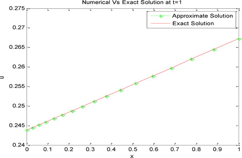
Table 1a. The MAEs at $t=1$ with ${\alpha }_0=0,\mathrm{}{\beta }_0=1,\mathrm{}{\gamma }_0=0.5,\mathrm{}\tau =1.6.$$h_l^2\left(\mathrm{Example}\mathrm{}1\right).$

Figure 2. The graph of approximate solution vs exact solution at $t=1(\mathrm{Example}\mathrm{}2).$ $(\eta =1,ϵ=0.01,\mathrm{}N+1=16,\mathrm{}\tau =1.6h_l^2)$

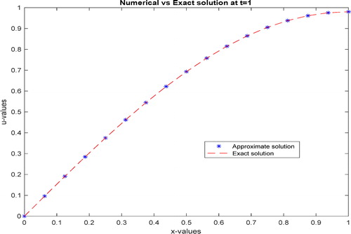
Table 1b. The MAEs at $t=1$ with ${\alpha }_0=1,\mathrm{}{\beta }_0=5,\mathrm{}{\gamma }_0=0.75,\mathrm{}\tau =1.6.$$h_l^2$ $\left(\mathrm{Example}\mathrm{}1\right).$

Figure 3. The graph of approximate solution vs analytical solution at $t=1(\mathrm{Example}\mathrm{}3).$ $(\eta =0.95,\mathrm{}{R}_e=10^6,N+1=16,\mathrm{}\tau =1.6h_l^2)$

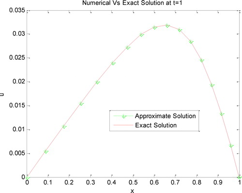
Table 1c. The MAEs at $t=1$ with ${\alpha }_0=5,\mathrm{}{\beta }_0=1,\mathrm{}{\gamma }_0=0.75,\mathrm{}\tau =1.6.$$h_l^2$ $\left(\mathrm{Example}\mathrm{}1\right).$

Table 2a. The MAEs at $t=1$ with $ϵ=0.1,\tau =1.6.$$h_l^2$ $\left(\mathrm{Example}\mathrm{}2\right).$

Figure 4. The graph of approximate solution vs analytical solution at $t=1(\mathrm{Example}\mathrm{}4).$ (R_e = 10, α = 2, N+1 = 50, τ = 0.01)

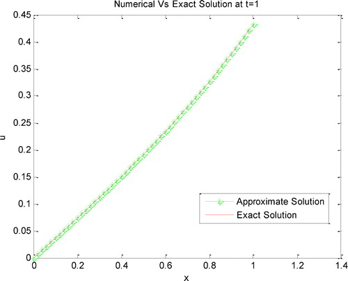
Table 4. The MAEs at $t=1,\eta =0.92,\mathrm{}\tau =0.01$ $(\mathrm{Example}\mathrm{}4).$

Table 5a. The MAEs at $t=1$ with $R_e=100,\mathrm{}\tau =3.2.$$h_l^2$ $\left(\mathrm{Example}\mathrm{}5\right).$

Table 5b. The MAEs at $t=1$ with $R_e=250,\mathrm{}\tau =3.2.$$h_l^2$ $\left(\mathrm{Example}\mathrm{}5\right).$

Table 6a. The MAEs at $t=1$ with $ϵ=0.01,\tau =1.6.$$h_l^2$ $\left(\mathrm{Example}\mathrm{}6\right).$

Figure 5. The graph of approximate solution vs exact solution at $t=1(\mathrm{Example}\mathrm{}5).$ (R_e = 100, N+1 = 16, τ = 3.2$h_l^2$)

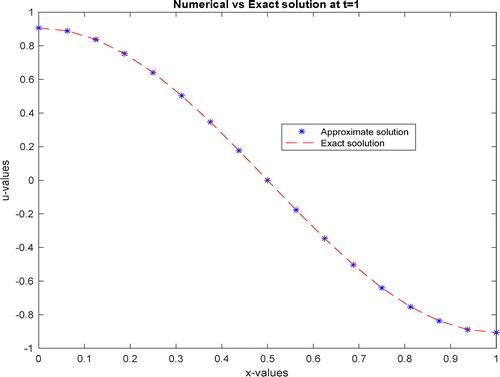
Table 2b. The MAEs at $t=1$ with $ϵ=0.01,\tau =1.6.$$h_l^2$ $\left(\mathrm{Example}\mathrm{}2\right).$

Figure 6. The graph of approximate solution vs exact solution at $t=1$ and t = 2 $(\mathrm{Example}\mathrm{}6).$ (ϵ = 0.01, N+1 = 16, τ = 3.2$h_l^2$)

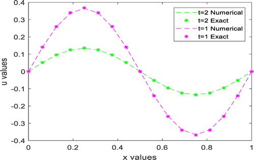
Table 3. The MAEs at $t=1$ with $\eta =0.95,$ $\tau =1.6.$$h_l^2$ $\left(\mathrm{Example}\mathrm{}3\right).$

Figure 7. Approximate vs analytical solutions at different time levels $(\mathrm{Example}\mathrm{}7).$

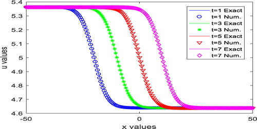
Table 7. The global relative errors $(\mathrm{Example}\mathrm{}7).$

Table 6b. The MAEs at $t=2$ with $ϵ=0.01,\tau =1.6.$$h_l^2$ $\left(\mathrm{Example}\mathrm{}6\right).$

Additional information

Funding

This research work is supported by Science and Engineering Research Board (SERB), Department of Science & Technology (DST), Government of India, Sanction Order No.: CRG/2018/004608.