Tutorial: The LuxPy Python Toolbox for Lighting and Color Science

ABSTRACT

LuxPy is a free and open source Python package that supports several common lighting, colorimetric, color appearance, and other color science related calculations that should be useful to researchers and industry professionals. This article describes the installation of the LuxPy toolbox, provides an overview of its basic design and functionality, and gives several examples to demonstrate its basic utilities using a Jupyter notebook. LuxPy is available under a GPLv3 license at www.github.com/ksmet1977/luxpy/ or from the Python Package Index pypi.python.org/pypi/luxpy/.

KEYWORDS:

• CCT
• chromatic adaptation
• color appearance
• colorimetry
• color rendering
• color science
• duv
• hyper-spectral image simulation
• lighting
• models
• photobiological quantities
• Python
• spectral optimization
• tristimulus values
• toolbox

1. Learning Outcomes

It is the intent that, after studying this article and its associated Jupyter notebook, that the reader will

1. be able to install the LuxPy package in a dedicated Python conda (virtual) environment;

2. be able to import the package in the Anaconda Spyder IDE or a Jupyter notebook;

3. have had an overview of the package’s basic design and functionality;

4. have gained practical experience and knowledge on how to use the LuxPy package to perform a variety of basic, and some more advanced, calculations related to lighting and color science.

Note that this is a tutorial on the LuxPy package, not on Python itself. Good basic tutorials can be found online. For suggestions, the reader is referred to the LuxPy github page.

2. Introduction

Researchers and industry professionals in lighting and color science related fields often need to make or share various kinds of common spectral or colorimetric calculations, such as interpolating spectral data following (CIE15-2004 2004) or determining its correlated color temperature (CCT), distance to the blackbody locus (Duv), and color rendering index (CRI).

Functions implementing such calculations are often implemented using Microsoft Excel (possibly in combination with Visual Basics for Applications) or Matlab (MathWorks Inc 2018), each with their own advantages and disadvantages.

Though Excel or some open-source variant (for example, LibreCalc, Document Foundation, 2018) is a great way to perform some simple calculations—with little or no learning curve—, graphically represent the results, and share them with colleagues or collaborators, Excel implementations can rapidly become very unwieldy and difficult to follow as the problem complexity and quantity of the data increase. In addition, spreadsheet-type calculators lack flexibility when existing calculations need to be adjusted or there is a need to work on different sized data sets. They also lack some basic functionality that often comes in handy when analyzing data or graphically representing results (for example, try making a three-dimensional plot of some L*a*b* data).

For more complex problems, code-based calculations using a high-level—quite easy to learn—scripting language, such as Matlab or Python (www.python.org), are much more flexible and easier to follow and comprehend. In addition, Matlab and Python come with a large set of toolboxes that support a wide variety of functionality. However, that functionality and ease of use come at a cost, at least with Matlab, because it requires a quite expensive yearly renewable license. Python, on the other hand, is free and open source and has lots of toolboxes for analysis and numerical computing (for example, Numpy); hence its growing popularity.

To facilitate lighting- and color science–related calculations and to foster scientific collaboration using a shared, free, easy-to-learn, and powerful high-level scripting language, the LuxPy package was developed in Python 3. In addition, LuxPy could be used in an academic or other teaching settings to help students develop a basic understanding of and practical skills in lighting and color science, while simultaneously learning the basics of the Python programming language.

This article describes the installation of the LuxPy toolbox and its basic design and functionality and provides several examples to demonstrate its usage. A Jupyter notebook (www.jupyter.org)—a document that contains live code, graphics, and text and that can be run in a browser—has also been created to help the interested reader exploring the LuxPy toolbox in practice.

3. LuxPy Installation

The easiest and recommended way of installing the LuxPy package is as follows:

1. First, install miniconda for Python 3 (≥3.5) by downloading the installer (from conda.io/miniconda.html) for your operating system. This installs the conda package manager and python. Make sure conda.exe can be found on the system path (if necessary, add it manually).

2. Next, create a conda virtual environment for Python version 3.6 or higher with a full Anaconda distribution by opening up a (Anaconda)

   Table

   command shell

   and typing the following one line of commands after the $-prompt:

   Table

   $ conda create --name py36python=3.6 anaconda

Note that Anaconda from Continuum Analytics is a free and open-source distribution of Python for scientific computing that eases package management and deployment (it contains a large set packages specifically aimed at scientific computation). Enthought Canopy is another option.

• Once installed, activate the virtual environment (this step must be done each time you want to use any of the packages installed in the environment) by typing:

  Table

  $ activate py36

• Install pip—installer for packages listed on the Python Package Index (pypi.python.org)—to the py36 conda virtual environment to ensure that any packages installed with pip will be installed to the py36 environment and not globally:

  Table

  (py36) $ conda install pip

• The LuxPy package can now be installed by typing:

  Table

  (py36) $ pip install luxpy

The LuxPy packages has several dependencies (SciPy, NumPy, Pandas, Matplotlib, scikit-image, and Setuptools). Should any errors show up, try to perform a manual install of these dependencies, using either, for example, “conda install scipy” or “pip install scipy,” and then try to reinstall luxpy using pip.

3.1. Use of LuxPy within the Spyder IDE

Spyder is an Interactive Development Environment (IDE) for scientific programming in the Python language. It supports IPython and popular Python libraries such as NumPy, SciPy, or matplotlib. It should come installed with the Anaconda distribution in the conda virtual environment. If not, it can be installed by typing:

Table

$ conda install -n py36 spyder

To start using LuxPy, open up the Spyder IDE in the py36 virtual environment:

Table

$ activate py36(py36) $ spyder

The Luxpy package can now be imported into a module (.py script file) or the global namespace in the Spyder IDE (command line) by typing:

import luxpy as lx

3.2. Use of LuxPy within a Jupyter Notebook

A Jupyter notebook (www.jupyter.org) is a document that can contain live code, graphics, and text and that can be run in a browser. It is therefore an easy way of sharing calculations and their results, while giving the user access to edit the code and rerun the calculations, perhaps with different inputs or parameters. The Jupyter notebook should come installed with the Anaconda distribution in the py36 virtual environment (if not, install it using “pip install jupyter”) and can be run as follows:

Table

(py36) $ jupyter notebook

To start using LuxPy, open up a new or existing notebook (for example, the “luxpy_basic_usage.ipynb” notebook that can be downloaded from www.github.com/ksmet1977/luxpy) and, as before, import the package by typing:

import luxpy as lx

4. LuxPy Design and Functionality

The LuxPy package functionality is distributed among several subpackages and modules. Some subpackages/modules load within the LuxPy namespace, others, dedicated to a specific functionality, load within the subpackage/module namespace itself and should be accessed through that name. A full description of all functions and their input arguments in the current version of LuxPy is beyond the scope of this article, which only addresses the basic usage of the package. A detailed description of each function’s input and output can be obtained in the usual way, by typing:

?lx.spd_to_xyz

to get help on, for example, the spd_to_xyz() function.

An overview with a short description of all functions in the LuxPy package can be found at: ksmet1977.github.io/luxpy or in the LuxPy_Documentation.pdf.

4.1. Package Structure and Functionality

The LuxPy toolbox contains a variety of subpackages (folder/subfolder/) and modules (.py) providing support for a number of basic and more advanced calculations related to lighting and color science. They are listed in Table 1 and on ksmet1977.github.io/luxpy and are briefly reviewed in the following subsections.

Table 1. Overview of structure of the subpackages/modules in the LuxPy package.

#	Subpackage(s)	Module(.py)	Namespace
1. utils	.helpers		luxpy
		helpers.py
	.math		luxpy.math
		math.py
		optimizers.py
2. spectrum	.spectral		luxpy
		cmf.py
		spectral.py
		spectral_databases.py
3. color	.ctf		luxpy
		colortransformations.py
		colortf.py
	.cct		luxpy
		cct.py
	.cat		luxpy.cat
		chromaticadaptation.py
	.cam		luxpy.cam
		colorappearancemodels.py
		cam_02_X.py
		cam15u.py
		sww2016.py
	.deltaE		luxpy.deltaE
		colordifferences.py
	.cri		luxpy.cri
		colorrendition.py
	.cri.utils	DE_scalers.py
		helpers.py
		init_cri_defaults_database.py
		graphics.py
	.cri.indices	indices.py
		cie_wrappers.py
		ies_wrappers.py
		cri2012.py
		mcri.py
		cqs.py
	.cri.iestm30	ies_tm30_metrics.py
		ies_tm30_graphics.py
	.cri.VFPX	VF_PX_models.py	luxpy.cri.VFPX
		vectorshiftmodel.py
		pixelshiftmodel.py
	.color.utils		luxpy
		plotters.py
4. classes			luxpy
		SPD.py (class SPD)
		CDATA.py (classes CDATA, XYZ, LAB)
5. toolboxes	.photbiochem		luxpy.photbiochem
		cie_tn003_2015.py
		ASNZS_1680_2_5_1997_COI.py
		circadian_CS_CLa_lrc.py
	.indvcmf		luxpy.indvcmf
		individual_observer_cmf_model.py
	.spdbuild		luxpy.spdbuild
		spd_builder.py
	.hypspcim		.luxpy.hypspcim
		hyperspectral_img_simulator.py

4.1.1. utils/helpers/

• helpers.py: Module with helper functions.

4.1.2. utils/math/

• math.py: Module with math functions.

• optimizers.py: Module for bounded optimization: minimizebnd().

4.1.3. spectrum/spectral/

• cmf.py: Module with Color Matching Functions and related.

• spectral.py: Module with spectral data related functions: e.g., spd_to_xyz(), spd_to_power(), cie_interp(), spd_normalize(), blackbody(), daylightphase(), cri_ref(), …

• spectral_databases.py: Module with spectral data: for example, CIE Reference Illuminants, CIE TCS reflectance functions, IESTM30 spectral functions, …

4.1.4. color/ctf/

• colortransforms.py: Module with color transformation functions: e.g., xyz_to_Yxy(), Yxy_to_xyz(), xyz_to_lab(), lab_to_xyz(),…

• colortf.py: Module enabling easy, shorthand color transformation: e.g., lx.colortf(spd, tf = ‘spd>Yxy’) and lx.xyz_to_Yxy(lx.spd_to_xyz(spd)) are equivalent.

4.1.5. color/cct/

• cct.py: Module with xyz tristimulus value conversions to CCT and Duv.

4.1.6. color/cat/

• chromaticadaptation.py: Module supporting chromatic adaptation transforms (von Kries and RLAB).

4.1.7. color/cam/

• colorappearancemodels.py: Module with color appearance models.

  1. cam_02_X.py: Module with CIECAM02 based models. (Li et al. 2017; Luo et al. 2006; Moroney et al. 2002); for example, ciecam02, cam16, cam02ucs, cam16ucs/lcd/scd.

  2. cam15u.py: Module with color appearance models (CAMs) for unrelated self-luminous stimuli (Withouck et al. 2015).

  3. sww2016.py: Module with CAMs based on mapping of Munsell color system (Smet et al. 2016).

4.1.8. color/deltaE/

● colordifferences.py: Module with color difference formulas: e.g., DE_camucs(), DE2000(), DE_cspace()

4.1.9. color/cri/

• colorrendition.py: Module related to color rendition calculations: e.g., spd_to_cri(), spd_to_ciera(), spd_to_cierf(), spd_to_iesrf(), …

  1. DE_scalers.py: scaling functions for color difference DE to CRI conversion.

  2. helpers.py: basic functions and data for CRI calculations.

  3. indices.py: Module with wrapper functions for various cri measures.

     1. cie_wrappers.py: Module with CIE cri metrics (R_a, R_f) (CIE13.3-1995 1995; CIE224:2017 2017).

     2. ies_wrappers.py: Module with IES cri metrics (R_f, R_g) (David et al. 2015; IES 2015).

     3. cri2012.py: Module with CRI2012 metrics.(Smet et al. 2013).

     4. mcri.py: Module with memory color rendition index, R_m.(Smet et al. 2012).

     5. cqs.py: Module supporting Color Quality Scale (v7.5 & v9.0).(Davis and Ohno 2010).

  4. graphics.py: basic cri plotting functions.

  5. ies_tm30_metrics.py: specific functionality for IES TM30 meetrics.

  6. ies_tm30_graphics.py: specific graphic support for IES TM30.

  7. VF_PX_models.py.

     1. vectorshiftmodel.py: support for vector field color shift and metameric uncertainty indices.

     2. pixelshiftmodel.py: supports color space pixel-based color shift calculations.

4.1.10. color/utils/

● plotters.py: Module with basic plotting functions: for example, for spectrum, daylight, and blackbody loci, …

4.1.11. classes/

• SPD.py: Class wrapper (spectral power distribution, SPD) around basic spectral functionality.

• CDATA.py: Class wrappers around basic tristimulus value (class XYZ) and color space and color appearance model transformations (class LAB).

4.1.12. toolboxes/ciephotbio/

• cie_tn003_2015.py: Module for CIE photobiological quantities (α-opic irradiance and equivalent illuminance) (CIE-TN003:2015 2015).

• ASNZS_1680_2_5_1997_COI.py: Module for the calculation of the Cyanosis Observation Index. (AS/NZS1680.2.5 1997).

• circadian_CS_CLa_lrc.py: Module implementing the Circadian Stimulus (CS) and Circadian Light (CLa) indices developed by the RPI Lighting Research Center (Rea et al. 2012).

4.1.13. toolboxes/indvcmf/

• individual_observer_cmf_model.py: Module supporting Monte Carlo generation of individual observer cone fundamentals (lms-CMFs) (Asano 2016).

4.1.14. toolboxes/spdbuild/

• spd_builder.py: Module for building (simulating) and optimizing multicomponent spectra.

4.1.15. toolboxes/hypspcim/

• hyperspectral_img_simulator.py: Module for simulating hyperspectral images.

4.2. Data Structure

LuxPy global constants (which should not be changed, so use copy() or deepcopy() when necessary!) can be recognized throughout in that they start with ‘_’ and are in an all _CAPITALS format. These constants contain various parameters, settings or dictionaries with useful data; for example, lx._CIE_ILLUMINANTS is a Python dictionary (dict) containing spectral data of various CIE illuminants (CIE15-2004 2004).

Many LuxPy functions expect to receive their input data in specific formats. Two major data types can be distinguished: spectral data and colorimetric data.

4.2.1. Spectral data using numpy.ndarrays

Spectral data should be inputted to functions in a row-based format as NumPy.ndarrays, with the first row containing the wavelengths and subsequent rows the values of one or more spectra. When using the function helpers.getdata to read spectral data stored in .csv or other data files, the data in the file itself should be in a column format.

A NumPy.ndarray variable “spds” containing two spectra and with wavelengths ranging from 380 nm to 780 nm and with a 5-nm wavelength spacing, thus should have a shape of (3, 81).

As an example, see the following code, which creates two spectra, a blackbody radiator and a CIE daylight phase, both with a CCT of 4500 K and with the wavelength range specified above, and queries its shape (whereby the code is split over multiple lines using the ‘\’ line separator character):

import luxpy as lx spds = lx.cri_ref([4500,4500],\      ref_type = ['BB','DL'],\       wl3 = [380,780,5]) print(spds.shape) (3, 81)

4.2.2. Colorimetric data using numpy.ndarrays

Colorimetric data are represented using two- or three-dimensional NumPy.ndarrays. The colorimetric dimension—for example, X, Y, Z tristimulus values—is always on the last (highest) array axis.

For example, the tristimulus values of an equi-energy white point should have a shape (1, 3) and can be created as follows:

import numpy as np # import NumPy package

xyzE = np.array([[100., 100., 100.]])

An array with tristimulus values for N stimuli should thus have a shape (N, 3).

However, three-dimensional arrays are also valid. In this case, the first axis is assumed to refer to different reflectance/transmittance samples, the second axis to the light sources illuminating those samples, and the last axis again to the colorimetric dimension.

The following code generates, for example, the CIE 1931 2° X, Y, Z tristimulus values for the eight Munsell Test Colour Samples (TCS) used in the CIE 13.3-1995 color rendering index R_a (CIE13.3-1995 1995), when illuminated by the two light source spectra generated earlier; that is the 4500 K blackbody and daylight phase spectra.

# gets the 8 CIE TCS from a database:

TCS8 = lx._CRI_RFL['cie-13.3-1995']['8']

# calculate xyz:

xyz8 = lx.spd_to_xyz(spds,

         cieobs = '1931_2',\

         relative = True,\

         rfl = TCS8)

print(xyz8.shape)

(8, 2, 3)

As can be seen, the shape of the xyz8 variable is (8, 2, 3); i.e., (sample total, light source total, 3).

Many other LuxPy functions—for example, xyz_to_Yuv()—take as input either the 2D or 3D Numpy.ndarray with the X, Y, Z tristimulus data to perform further calculations. These functions always assume that the array axes are specified as above. The advantage is that it is easy to do calculations on a whole block of data at once, without the user having to specifically write loops to calculate the requested transformation for each sample and/or light source. For example:

# Calculate Y, CIE1976 u'v' chromaticity

# coordinates:

Yuv8 = lx.xyz_to_Yuv(xyz8)

# Convert back to tristimulus values:

xyz8_2 = lx.Yuv_to_xyz(Yuv8)

print(Yuv8.shape)

(8, 2, 3)

As a final example, consider the calculation of the CCT and Duv of a bunch of (in this case, the two specified above) light source spectra:

xyzw = lx.spd_to_xyz(spds,

         cieobs = '1931_2',\

         relative = True,\

         rfl = None)

cct, duv = lx.xyz_to_cct(xyzw,

         cieobs = '1931_2',\

         mode = 'ohno',\

         out = 2)

print(cct.shape)

(2, 1)

4.2.3. Spectral and colorimetric data using LuxPy classes

Spectral and colorimetric data also have their own dedicated classes that have basic functionality by providing class method wrappers to some of the LuxPy functions.

An instance of the class SPD can be created by initiating it directly with a NumPy.ndarray or by providing the path to a datafile as input. Using the “spds” data array specified above (containing blackbody radiator and daylight phase spectra of 4500 K):

spds_inst = lx.SPD(spds)

The advantage of the creating such an SPD instance is that it allows for very readable code, when performing several operations in sequence:

xyz_inst = lx.SPD(spds).cie_interp(wl_new = [400, 700, 5]).to_xyz()

The code above produced an instance of class XYZ, xyz_inst, which itself has several methods for easy use. It is also easy to store some additional specific info related to the data:

print(“*Spectral data type in .dtype field: {}”.format(spds_inst.dtype))

print(“*Wavelengths in .wl field: {}”.format(spds_inst.wl.shape))

print(“*Values in .value field: {}”.format(spds_inst.value.shape))

print(“*Number of spds in .N field: {}”.format(spds_inst.N))

print(“*Shape of .value in .shape field: {}”.format(spds_inst.shape))

Output:

*Spectral data type in .dtype field: S

*Wavelengths in .wl field: (81,)

*Values in .value field: (2, 81)

*Number of spds in .N field: 2

*Shape of .value in .shape field: (2, 81)

The further conversion to CIELUV L*u*v* coordinates, with assumed white point the equi-energy white, can, for example, be done as follows:

luv_inst = xyz_inst.ctf(dtype = 'luv',\

 xyzw = np.array([[100, 100, 100]]))

In each instance, the field “value” contains the actual data. For the SPD class, this is the spectral data stripped of its wavelengths (contained in a “wl” field); for the XYZ and LAB classes, this is an array with the tristimulus values and specified colorimetric data, respectively. For the latter a field called “dtype” keeps track of what type of data (for example, “xyz,” “Yuv,” “luv,” …) the instance contains. In addition to a field “cieobs,” which specifies the color matching functions (CMF) set used, instances of the class LAB also contain a field “cspace_par” that contains a Python dictionary with a set of parameters (for example, “xyzw”) relevant to the calculation of the colorimetric values.

# Print data in parameter dictionary: print(luv_inst.cspace_par)

Output:

{'cieobs': '1931_2',

'xyzw': array([[100, 100, 100]]),

'M': None,

'scaling': None,

'Lw': None,

'Yw': None,

'Yb': None,

'conditions': None,

'yellowbluepurplecorrect': None,

'mcat': None,

'ucstype': None,

'fov': None,

'parameters': None}

Each class also contains a basic plotting method for a quick look at the data contained in the instance:

spds_inst.plot() #class SPD

xyz_inst.plot() #class XYZ

xyz_inst.ctf(dtype = 'Yuv').plot(plt_type

= '2d', title =“CIE u'v'”) #class LAB

lx.plotSL() # plots spectrum locus

The output of the first and last two commands is illustrated in respectively the top and bottom graphs of Fig. 1.

4.3. Versioning System

Each release of LuxPy is tagged with a MAJOR.MINOR.PATCH version number following the principles of semantic versioning whereby the MAJOR number reflects changes in the LuxPy package that break compatibility with previous versions, the MINOR number reflects changes that add functionality or that are backward compatible, and the PATCH number reflects bug fixes or minor additions.

The current version associated with this article is LuxPy_v1.3.10.

5. Example Usage

In this section, the basic use of the LuxPy package will be demonstrated with the help of a Jupyter notebook, “luxpy_basic_usage.ipynb,” which can be downloaded from www.github.com/ksmet1977/luxpy.

5.1. Importing LuxPy and Other Python Packages

Any session would start with importing the necessary packages.

# Package for color science calculations: import luxpy as lx

# Package for scientific computing:

import numpy as np

# Package for plotting:

import matplotlib.pyplot as plt

# Package for timing functions:

import timeit

# Ensure inline plotting of figures:

%matplotlib inline

Note that getting help on a function or module is as easy as typing:

# get help on function arguments:

?lx.spd_to_xyz

# get help on cri sub-package:

?lx.cri

5.2. Working with Spectral Data

5.2.1. cri_ref()

As a first example, let us get (M = 4) spectra normalized at wavelength (“lambda”) 560 nm with respective CCTs of 3000 K, 4000 K, 4500 K, and 6000 K and respective types: “BB” (blackbody radiator), “DL” (daylight phase), “cierf” (mixed reference illuminant as defined in CIE224:2017[2017]), and “BB”:

# Set CIE observer, i.e. cmf set:

cieobs = '1964_10'

# Define M = 4 CCTs:

ccts = [3000,4000,4500, 6000]

# Define reference illuminant types

ref_types = ['BB','DL','cierf','DL']

# Calculate reference illuminants:

REF = lx.cri_ref(ccts, \

        ref_type = ref_types,\

        norm_type = 'lambda',\

        norm_f = 600)

print('* REF.shape --> (M + 1 x number of wavelengths): {}'.format(REF.shape))

Output:

* REF.shape --> (M + 1 x number of

wavelengths): (5, 471)

5.2.2. cie_interp()

Secondly, let us interpolate the REF spectral data to a 400 nm–700 nm range with a 5-nm spacing, and let the cie_interp() function determine the right kind of interpolation by defining the spectral data type as kind = 'S':

REFi = lx.cie_interp(REF, \

  wl_new = np.arange(400,700+1,5),\

   kind = 'S')

print('* REFi.shape --> (M + 1 x number of wavelengths): {}'.format(REFi.shape))

Output:

* REFi.shape --> (M + 1 x number of

wavelengths): (5, 61)

5.2.3. Spd_to_xyz()

Next, the tristimulus values (using the CIE 1964 10° CMFs) of those light source spectra can be obtained as follows:

# Get illuminant xyz:

xyz_REF = lx.spd_to_xyz(REF, \

            cieobs = cieobs)

The tristimulus values of set of N reflective samples illuminated by those M sources can be obtained in the following way:

# Get 8 TCS from CIE 13.3-1995:

TCS8 = lx._CRI_RFL['cie-13.3-1995']['8']

# Get TCS xyz:

xyz_TCS8_REF = lx.spd_to_xyz(REF, \

           cieobs = cieobs,\

           rfl = TCS8, \

           relative = True)

whereby relative = True (default) specifies that the output tristimulus values are normalized such that a perfect white diffuse sample has Y = 100.

The tristimulus values of the N samples illuminated by the M light sources and of the M light sources themselves can be obtained using:

xyz_TCS8_REF_2, xyz_REF_2 =

   lx.spd_to_xyz(REF,\

           cieobs = cieobs,\

           rfl = TCS8,\

           relative = True,\

           out = 2)

print('* xyz_TCS8_REF_2.shape -->

(NxMx3): {}'.format(xyz_TCS8_REF_2.shape))

print('* xyz_REF_2.shape -->

(Mx3):}'.format(xyz_REF_2.shape))

Output:

* xyz_TCS8_REF_2.shape --> (NxMx3):

(8, 4, 3)

* xyz_REF_2.shape --> (Mx3): (4, 3)

5.2.4. Plotting

A simple plot (see Fig. 2) of the spectral data in REF can be made by the following lines of code:

Fig. 1. Output as generated by the plot() methods of classes SPD (top) and LAB (bottom).

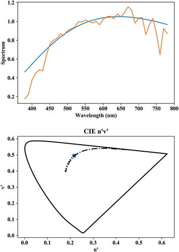
Fig. 2. Plot of spectral data in REF.

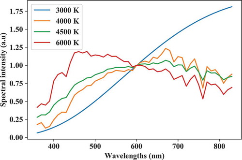
plt.plot(REF[0],REF[1:].T)

plt.xlabel('wl (nm)')

plt.ylabel('spectral intensity (a.u)')

lgnd_str = ['{} K'.format(x) for x in ccts]

plt.legend(lgnd_str)

Figures can be easily exported for use in presentations and publications using the matplotlib function figsave():

# Save figure in TIFF format at 600 dpi:

plt.figsave('Fig1_REF_spectra.tif',\

       format = 'tiff',\

       dpi = 600)

5.2.5. Individual observer color matching functions

Color matching functions are stored in a dictionary that can be accessed as follows:

# Get CIE 1931 2° CMFs:

cmf_1931 = lx._CMF['1931_2']['bar']

# List all available CMF sets:

print(lx._CMF['types'])

Output:

['1931_2','1964_10','2006_2','2006_10','1931_2_judd1951',

'1931_2_juddvos1978','1951_20_scotopic']

There is also a module, called “indvcmf,” that supports Monte Carlo generation of individual observer cone fundamentals and XYZ color matching functions (Asano 2016). For example, a set of cone fundamentals (lms) for a stimulus with field size of 6° for 20 observers aged 32 can be generated as follows:

# Get 20 individual observer lms-CMFs:

lmsb =

 lx.indvcmf.genMonteCarloObs(n_obs = 20,\

           list_Age = [32],\

           fieldsize = 6)

# Or, using US 2010 population census# to generate Age Distribution,

# and output as XYZ CMF:

xyzb_us =

 lx.indvcmf.genMonteCarloObs(n_obs = 20,\

       list_Age = 'us_census',\

         fieldsize = 6,\

         out ='XYZ')

The graph in Fig. 3 was generated by:

Fig. 3. Monte Carlo–generated individual XYZ color matching functions.

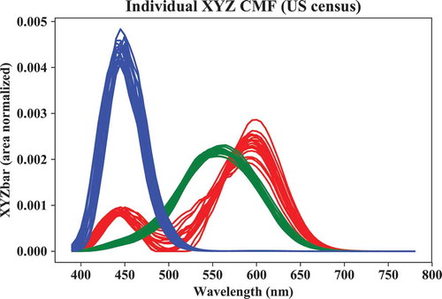
# Plot CMFs:

plt.figure()

plt.plot(xyzb_us[0],xyzb_us[1],\

     color ='r', linestyle ='-')

plt.plot(xyzb_us[0],xyzb_us[2],\

     color ='g', linestyle ='-')

plt.plot(xyzb_us[0],xyzb_us[3],\

     color ='b', linestyle ='-')

plt.xlabel('Wavelength (nm)')

plt.ylabel('XYZbar (area normalized)')

plt.title('Individual XYZ CMF (US census)')

The XYZ values, using the Monte Carlo–generated CMFs, for spectral data in REF can be calculated as follows:

# Calculate XYZ values for REF:

xyz_ind = np.empty((REF.shape[0] - 1,\

xyzb_us.shape[-1],3))

for i in range(xyzb_us.shape[-1]):

  xyz_ind[:,i,:] = lx.spd_to_xyz(REF,\

      cieobs = xyzb_us[…,i],\

      relative = True)

print(xyz_ind.shape)

Output:

(4, 20, 3)

Categorical observer CMFs can be generated in a similar manner using the indvcmf.genCatObs function.

5.3. Working with Colorimetric Data

The tristimulus values XYZ obtained earlier can be further transformed to a range of color coordinates.

5.3.1. xyz_to_Yuv()

As an example, the transformation to the CIE 1976 u’v’ chromaticity coordinates is outlined below:

Yuv_REF_2 = lx.xyz_to_Yuv(xyz_REF_2)

Yuv_TCS8_REF_2 = lx.xyz_to_Yuv(xyz_TCS8_REF_2)

print(“* Yuv_REF_2.shape --> (Mx3):{}”.format(Yuv_REF_2.shape))

print(“* Yuv_TCS8_REF_2.shape --> (NxMx3):{}”.format(Yuv_TCS8_REF_2.shape))

Output:

* Yuv_REF_2.shape --> (Mx3): (4, 3)

* Yuv_TCS8_REF_2.shape --> (NxMx3):

8, 4, 3)

5.3.2. asplit(), plotSL() and plot_color_data()

The colorimetric data can also be easily plotted. First the spectrum locus is drawn using plotSL(). This function has several input options (cspace and cieobs respectively determine the color space and CMF set to be used, show = False waits with showing the output graph until everything has been drawn in the axh axes, and BBL = True and DL = True regulate the plotting of a blackbody and daylight locus).

axh = lx.plotSL(cspace = 'Yuv',\

         cieobs = cieobs,\

         show = False,\

         BBL = True,\

         DL = True)

In a next step, the data are prepared for easy plotting by splitting the data array along the colorimetric dimension (last axis) and squeezing out any axes with a one-dimensional size:

# Split array along last axis:

Y, u, v = np.squeeze(lx.asplit(Yuv_REF_2))

Finally, to plot the u’, v’ chromaticity coordinates (see Fig. 4):

Fig. 4. Output of plot_color_data().

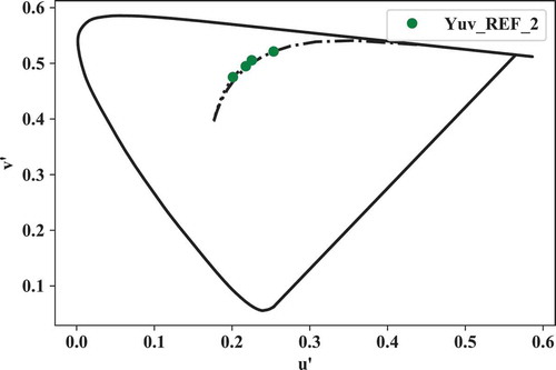
lx.plot_color_data(u,v, formatstr = 'go',\

        label = 'Yuv_REF_2')

5.3.3. colortf() and _CIE_ILLUMINANTS

A shorthand color transformation function also exists. This function makes it easy to combine several transformations in one function call.

In the following example, tristimulus values XYZ are transformed to CIE 1976 u’v’ chromaticity coordinates (tf = 'Yuv' defines the type of transform):

Yuv_REF = lx.colortf(xyz_REF_2, \

            tf = 'Yuv')

Note that the input does not have to be an array with tristimulus values. One can also perform a transformation between, for example, an array with spectral data and CIE 1976 u’v’ chromaticity coordinates. Any combination of transformations for which the necessary forward (xyz_to_…) and backward (…_to_xyz) functions are defined can be made. For example, the spectral data in REF can be readily converted to colorimetric data by specifying the correct transform type (tf = 'spd>Yuv'):

Yuv_REF = lx.colortf(REF,\

            tf = 'spd>Yuv')

Some color transformations require additional input parameters. This can be supplied as a Python dictionary with the parameter names as keys. The forward and backward transform parameters should be supplied to the colortf function using keyword arguments fwtf and bwtf, respectively.

For example, let us transform the Yuv_REF to CIE 1976 CIELAB L*a*b* coordinates, with as white point tristimulus values those of CIE illuminant A. First, the dictionary with input parameters for the forward (i.e., xyz_to_lab) transform is defined:

xyzwA =

lx.spd_to_xyz(lx._CIE_ILLUMINANTS['A'])

fwtf_userdefined = {'xyzw' : xyzwA}

whereby the spectrum of the CIE illuminant A is obtained from a LuxPy database with CIE illuminants; that is, _CIE_ILLUMINANTS.

Next, the transform can be made as follows:

lab_REF2 = lx.colortf(Yuv_REF_2,\

       tf = 'lab',\ fwtf = fwtf_userdefined)

Input parameters for the forward (only) transform can also be directly entered as keyword arguments to the colortf function:

lab_REF2 = lx.colortf(Yuv_REF_2, \

             tf = 'lab',\

             xyzw = xyzwA)

5.3.4. Xyz_to_cct() and cct_to_xyz()

The CCT and Duv can be obtained using Ohno’s method (Ohno 2014) or using a brute-force search method in the CIE 1960 Uniform Color Space (UCS) as follows:

# Ohno's approach with a Look-Up-Table:

cct_ohno, duv_ohno =

    lx.xyz_to_cct(xyz_REF_2,\

           cieobs = cieobs,\

           out = 'cct,duv',\

           mode = 'lut')

# Brute-force search approach:

cct_search, duv_search =

      lx.xyz_to_cct(xyz_REF_2,\

           cieobs = cieobs,\

           out = 'cct,duv',\

           mode = 'search')

whereby cieobs is a specifier for the type of CMFs that were used to calculate the tristimulus input values, out specifies the format of the output, and mode determined the method used to obtain the CCT and Duv.

To perform the inverse calculation—that is, going from CCT and Duv to tristimulus values,

# Ohno's approach with a Look-Up-Table:

xyz_REF_2_ohno =

      lx.cct_to_xyz(cct_ohno,\

           duv = duv_ohno,\

           cieobs = cieobs,\

           mode = 'lut')

# Brute-force search approach:

xyz_REF_2_search =

     lx.cct_to_xyz(cct_search,\

           duv = duv_search,\

           cieobs = cieobs,\

           mode = 'search')

Note that the brute-force method takes considerably longer than Ohno’s method:

print('\nRun-time: cct_to_xyz_ohno():')

%timeit xyz_REF_2_ohno =

 lx.cct_to_xyz(cct_ohno,         duv = duv_ ohno,\

        cieobs = cieobs,         mode = 'lut')

print('\nRun-time: cct_to_xyz_search():')

%timeit xyz_REF_2_search =

lx.cct_to_xyz(cct_search,

         duv = duv_search,\

         cieobs = cieobs,\

         mode = 'search')

Output:

Run-time: cct_to_xyz_ohno():

84.8 ms ± 1.14 ms per loop (mean ± std. dev. of 7 runs, 10 loops each)

Run-time: cct_to_xyz_search():

10.1 s ± 167 ms per loop (mean ± std. dev. of 7 runs, 1 loop each)

Please be aware that running the above code block could take a while, because the timeit macro needs to execute the cct_to_xyz() function several times.

5.4. Chromatic Adaptation and Corresponding Colors (.cat)

LuxPy supports basic von Kries-type chromatic adaptation transforms, with a wide choice of sensor spaces (for example, CAT02, CMC2000, et cetera; for an overview, see lx.cat._MCATS) and several degrees of adaptation formulas.

As an example, let us calculate the corresponding colors under CIE illuminant D65 (xyzw2) of the eight CIE TCS illuminated by the spectra in REF (xyzw1) using a two-step (catmode = '1>0>2') chromatic adaptation transform (Smet et al. 2017) with CAT02 sensors and with an assumed adapting field luminance, La, of respectively 100 cd/m² and 500 cd/m²:

# Original illumination condition:

xyzw1 = xyz_REF

# New illumination condition:

D65 = lx._CIE_ILLUMINANTS['D65']

xyzw2 = lx.spd_to_xyz(D65,\

           cieobs = cieobs,\

           relative = True)

# Apply von Kries CAT:

xyz_TCS8_REFc= lx.cat.apply(xyz_TCS8_REF,\

       xyzw1 = xyzw1,\

       xyzw2 = xyzw2,\

       catmode = '1>0>2',\

       cattype='vonkries',\

       D = None,\

       La = np.array([[100,500]]))

The original and corresponding colors can be plotted (see Fig. 5) as follows:

Fig. 5. Plot of u’v’ coordinates of CIE TCS8 before (red circles) and after (blue diamonds) a von Kries CAT from a 3000 K blackbody radiator to CIE illuminant D65.

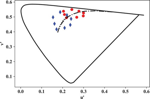
# convert to CIE 1976 u'v':

Yuv_TCS8_REF =

 lx.xyz_to_Yuv(xyz_TCS8_REF)

Yuv_TCS8_REFc =

 lx.xyz_to_Yuv(xyz_TCS8_REFc)

# create figure with 1 axes:

ax = plt.figure().add_subplot(111)

ax.plot(Yuv_TCS8_REF[:,0,1],\

     Yuv_TCS8_REF[:,0,2],\

     color ='r',\

     marker = 'o',\

     linestyle = 'none')

ax.plot(Yuv_TCS8_REFc[:,0,1],\

     Yuv_TCS8_REFc[:,0,2],\

     color ='b',\

     marker ='d',\

     linestyle = 'none')

ax.set_xlabel(“u'”) # set x-axis label

ax.set_ylabel(“v'”) # set y-axis label

# Plot spectrum, BB and DL loci:

lx.plotSL(cieobs = cieobs,\

     cspace = 'Yuv', \

     DL = True, \

     BBL = True)

5.5. Color Appearance Models (.cam)

Several CAMs, such as CIECAM02 (Moroney et al. 2002), CAM02-UCS/LCD/SCD (Luo et al. 2006), CAM16 and CAM16-UCS/LCD/SCD (Li et al. 2017), CAM15u (Withouck et al. 2015), and CAMSWW2016 (Smet et al. 2016), have been implemented. In this section, the use of the xyz_to_jab… type wrapper functions will be demonstrated.

For example, let us look at the conversion from XYZ tristimulus value to CIECAM02 J, a_M, b_M coordinates and plot the results in Fig. 6 (similar functionality is supported for the other CAMs):

Fig. 6. Plot of CIE TCS8 samples in CIECAM02 J, a_M, b_M. Red circles: default viewing conditions, blue diamonds: user-defined conditions.

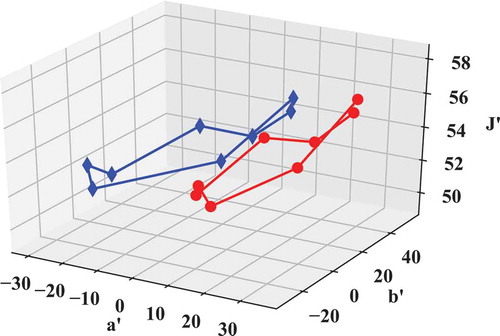
# Use default conditions

# (see lx.cam._CAM_DEFAULT_CONDITIONS):

JabM_TCS8_REF =

lx.xyz_to_jabM_ciecam02(xyz_TCS8_REF)

# Create a dictionary with user defined viewing conditions:

usr_cnds = {'D': None,\

          'Dtype': None,\

          'La': 500.0,\

          'Yb': 40.0,\

          'surround': 'dim'}

JabM_TCS8_REF_user =

 lx.xyz_to_jabM_ciecam02(xyz_TCS8_REF,\

        xyzw = xyz_REF,\

        conditions = usr_cnds)

# Plot color coordinates in a 3d graph:

ax = plt.figure()

ax.add_subplot(111,projection = '3d')

ax.plot(JabM_TCS8_REF[:,0,1],\

     JabM_TCS8_REF[:,0,2],\

     JabM_TCS8_REF[:,0,0],\

     color = 'r', marker = 'o')

ax.plot(JabM_TCS8_REF_user[:,0,1],\

     JabM_TCS8_REF_user[:,0,2],\

     JabM_TCS8_REF_user[:,0,0], \

     color ='b', marker ='d')

ax.set_zlabel(“J'”)

ax.set_xlabel(“a'”)

ax.set_ylabel(“b'”)

5.6. Color Difference Calculation (.deltae)

The deltaE subpackage supports calculation of color differences in various color spaces or color appearance spaces.

The widely used DE2000 color difference formula (Sharma et al. 2005) has been implemented and supports direct input of tristimulus values or CIE 1976 L*a*b* color coordinates. For example, let us calculate the color difference between the color samples illuminated by the first and last spectrum in REF.

# Calculate DE2000:

DE00 =

 lx.deltaE.DE2000(xyz_TCS8_REF[:,0,:], \

        xyz_TCS8_REF[:,-1,:],\

        xyzwt = xyz_REF[:1,:],\

         xyzwr = xyz_REF[-1:,:])

# Calculate DE2000,

# and also output rms average (DE00a),

# use default KLCH scaling factors:

DE00i, DE00a =

 lx.deltaE.DE2000(xyz_TCS8_REF[:,0,:],\

       xyz_TCS8_REF[:,-1,:],\

       xyzwt = xyz_REF[:1,:],\

       xyzwr = xyz_REF[-1:,:],\

       avg = lx.math.rms, \

       out = 'DEi,DEa', \

       KLCH = [1,1,1])

# Calculate DE2000,

# and also output rms average (DE00a),

# but ignore L*,

# and double the kC scaling factor:

DE00i_ab, DE00a_ab =

  lx.deltaE.DE2000(xyz_TCS8_REF[:,0,:],\

      xyz_TCS8_REF[:,-1,:],\

      xyzwt = xyz_REF[:1,:],\

      xyzwr = xyz_REF[-1:,:],\

      avg = lx.math.rms,\

      out = 'DEi,DEa',\

      KLCH = [1,2,1],\

      DEtype = 'ab')

The function DE_camucs supports calculation of color differences in color appearance spaces (CIECAM02, CAM16, CAM02ucs, CAM16lcd, …):

# Calculate DE in CIECAM02

# using default CAM viewing conditions:

DEi_ciecam02 =

 lx.deltaE.DE_camucs(xyz_TCS8_REF[:,0,:],\

      xyz_TCS8_REF[:,-1,:],\

      xyzwt = xyz_REF[:1,:],\

      xyzwr = xyz_REF[-1:,:],\

      out ='DEi', \

      camtype = 'ciecam02',\

      ucstype = 'none')

# DE in CAM02-ucs (def. CAM viewing conds.)

DEi_cam02ucs =

 lx.deltaE.DE_camucs(xyz_TCS8_REF[:,0,:],\

      xyz_TCS8_REF[:,-1,:],\

      xyzwt = xyz_REF[:1,:], \

      xyzwr = xyz_REF[-1:,:],\

      out ='DEi', \

      camtype = 'ciecam02', \

      ucstype = 'ucs')

# DE in CAM16-lcd (def. CAM viewing conds.)

DEi_cam16lcd =

 lx.deltaE.DE_camucs(xyz_TCS8_REF[:,0,:],\

       xyz_TCS8_REF[:,-1,:],\

       xyzwt = xyz_REF[:1,:],\

       xyzwr = xyz_REF[-1:,:],\

       out ='DEi',\

       camtype = 'cam16',\

       ucstype = 'lcd')

A handy function, DE_cspace(), exists that can calculate DE2000, CAMUCS-type color differences but also color differences in any color space or chromaticity diagram for which the function xyz_to_… is defined. The input arguments are as before, with the additional argument “tf” specifying the color difference type (that is, “DE2000” or “camucs”) or color space (for example, “Yuv” or “lab”). When “tf” is different from “DE2000” or “camucs,” there is the possibility of using the KLCH argument to specify different weights for the lightness, chroma, and hue dimensions.

# DE2000:

DEi_2000 =

 lx.deltaE.DE_cspace(xyz_TCS8_REF[:,0,:],\

       xyz_TCS8_REF[:,-1,:],\

       xyzwt = xyz_REF[:1,:],\

       xyzwr = xyz_REF[-1:,:],\

       out = 'DEi',\

       tf = 'DE2000')

# DE CAM02-ucs:

DEi_cam02ucs =

 lx.deltaE.DE_cspace(xyz_TCS8_REF[:,0,:],\

       xyz_TCS8_REF[:,-1,:],\

       xyzwt = xyz_REF[:1,:],\

       xyzwr = xyz_REF[-1:,:],\

       out = 'DEi',\

       camtype = 'ciecam02',\

       ucstype = 'ucs',\

       tf = 'camucs')

# DE CIE 1976 L*a*b*:

DEi_lab =

 lx.deltaE.DE_cspace(xyz_TCS8_REF[:,0,:],\

       xyz_TCS8_REF[:,-1,:],\

       xyzwt = xyz_REF[:1,:],\

       xyzwr = xyz_REF[-1:,:],\

       out = 'DEi',\

       tf = 'lab')

# DE CIE 1976 L*a*b*

# with kL, kC and kH weights different from

# unity (KLCH = [2,3,4]):

DEi_lab_KLCH =

 lx.deltaE.DE_cspace(xyz_TCS8_REF[:,0,:],\

       xyz_TCS8_REF[:,-1,:],\

       xyzwt = xyz_REF[:1,:],\

       xyzwr = xyz_REF[-1:,:],\

       out = 'DEi',\

       tf = 'lab',\

       KLCH = [2,3,4])

5.7. Color Rendition Measures (.cri)

The .cri subpackage supports several color rendition metrics, such as CIE13.3-1995 R_a (CIE13.3-1995 1995), CIE224-2017 R_f (CIE224:2017 2017), IESTM30 R_f and R_g (David et al. 2015; IES 2015), CRI2012 (Smet et al. 2013), Memory Color Rendition Index (MCRI) (Smet et al. 2012), and Color Quality Scale (CQS) (Davis and Ohno 2010). It also contains handy functions to construct new color fidelity-type metrics very easily by changing, for example, the sample set, averaging method, color space, CIE observer, et cetera.

Finally, a subpackage cri.VFPX also supports the calculation of vector field–based and pixel-based color shifts, of a metameric uncertainty index, et cetera.

Wrapper functions have been created specifically dedicated to the standard definition of the published color rendition measures:

# Get some spectra from the IESTM30 light

# source database:

N = 4

spds = lx._IESTM3015['S']['data'][:N+1]

# CIE13.3-1995 Ra:

ciera = lx.cri.spd_to_ciera(spds)

# CIE224-2017 Rf:

cierf = lx.cri.spd_to_cierf(spds)

# IES-TM30-15 Rf:

iesrf_15 = lx.cri.spd_to_iesrf(spds,\

     cri_type = 'iesrf-tm30-15')

# IES-TM30-15 Rg:

iesrg_15 = lx.cri.spd_to_iesrg(spds,\

     cri_type = 'iesrf-tm30-15')

# IES-TM30-18 Rf:

iesrf_18 = lx.cri.spd_to_iesrf(spds)

# IES-TM30-18 Rg:

iesrg_18 = lx.cri.spd_to_iesrg(spds)

The use of the more versatile spd_to_cri function allows the calculation of a color fidelity value using all of the same standard parameters as those of the metric defined in cri_type but with, for example, a change of the sample set from the IES99 to the IES4880, using a blackbody radiator as reference illuminant and using the rms instead of the mean to average the color differences before calculating the general color fidelity index. Requested output can be specified by out:

# Get IES 4880 reference set:

R = lx._CRI_RFL['ies-tm30']['4880']['5nm']

# Calculate custom Rf & Rg

# and cct & duv:

Rf_custom, Rg_custom, cct, duv =

     lx.cri.spd_to_cri(spds,\

     cri_type = 'ies-tm30',\

     out = 'Rf,Rg,cct,duv',\

     avg = lx.math.rms,\

     sampleset = R,\

     ref_type = 'BB')

The LuxPy.cri subpackage also supports a function that calculates several color rendition index values and provides TM30-like graphical output. For example, the code below generates the output in Fig. 7.

Fig. 7. TM30-like graphic output of the color rendition properties of CIE illuminant F4. Top left: SPD with inline text of CCT, Duv, R_f, R_g, and R_t (metameric uncertainty index). Mid row, left: R_fhi index values for hue bins 1–16. Mid row, right: same but base color shifts predicted by a vector field model. Bottom row left and right: local hue hue and chroma shifts. Top right: color graphic icon. Bottom right: base color shifts predicted by a vector field model together with the Munsell-5 hue lines.

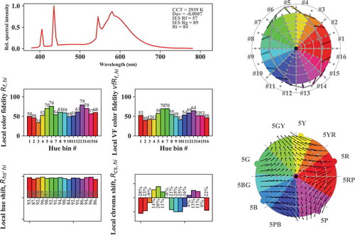
# Calculate and plot IES TM30

# color rendition measures:

SPD = lx._CIE_ILLUMINANTS['F4']

data,_,_ = lx.cri.plot_cri_graphics(SPD)

The output format of and displayed information in some of the right-hand graphs can be easily customized. For example, the graph in Fig. 8 was generated by the following code, which turns off the coloring of the right-hand-side color icons, plots the vector field base color shifts in grey and plots the distortion of the color gamut using circle fields (the color of the distorted circles provides information on the size of the hue shift, where red is larger):

Fig. 8. TM30-like graphic output of the color rendition properties of CIE illuminant F4. Similar to Fig. 7 but with hue coloring turned off in the right graphs and with base color shift vectors overlayed with lines representing the distortion of concentric chroma circles due to the specific color rendition properties of the test light source. Hue shift information is represented by the width and coloring of the lines: wider, more reddish lines represent larger hue shifts.

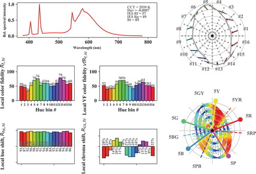
data = lx.cri.plot_cri_graphics(SPD,\

     plot_bin_colors = False,\

     vf_plot_bin_colors = False,\

     vf_color = 'grey',\

     plot_CF = True)

5.8. LuxPy Classes

The basic use of the SPD, XYZ and LAB classes has already been described in subsection 4.2.3 Spectral and colorimetric data using LuxPy classes. For further functionality, the reader is referred to the help in the __doc__ strings.

5.9. Calculation of Photobiological Quantities

Subpackage .photbiochem supports the calculation of various photobiological or related quantities, such as the Cyanosis Observation Index (COI) (AS/NZS1680.2.5 1997), the CIE photobiological quantities (α-opic irradiance and equivalent illuminance) defined in TN003:2015 (CIE-TN003:2015 2015; Lucas et al. 2014), or the Lighting Research Center’s CS and CLa (Rea et al. 2012) from spectral data.

Let us start with the TN003:2015 α-actinic quantities, for which a single dedicated function has been implemented: spd_to_aopicE(). The input spectral irradiance can be in W/m²∙nm (default) or in μW/cm²∙nm. The output is in SI units.

# Define a 4200 K blackbody radiator with

# a wavelength range between 378 nm and

# 782 nm, and a wavelength spacing of 1 nm:

BB = lx.blackbody(4200,\

       lx.getwlr([378,782,1]))

# Calculate the a-opic irradiance Eea

# and equivalent illuminance Ee

# for the blackbody radiator spectrum

# normalized to 100 lx:

Ees,Es = lx.photbiochem.spd_to_aopicE(BB,\

                E = 100)

# Print results:

print(“Photoreceptor cells:”)

print(lx.photbiochem._PHOTORECEPTORS)

print(“\na-opic irradiance symbols:”)

print(lx.photbiochem._Ee_SYMBOLS)

print(“a-opic irradiance values:”)

print(Ees)

print(“\na-opic illuminance symbols:”)

print(lx.photbiochem._E_SYMBOLS)

print(“a-opic illuminance values:”)

print(Es)

Output:

Photoreceptor cells:

['l-cone', 'm-cone', 's-cone','rod',

'iprgc']

a-opic irradiance symbols:

['Ee,lc','Ee,mc','Ee,sc','Ee,r','Ee,z']

a-opic irradiance values:

[[0.17140925 0.15161959 0.04969815 0.12215436 0.09792088]]

a-opic illuminance symbols:

['E,lc', 'E,mc', 'E,sc', 'E,r', 'E,z']

a-opic illuminance values:

[[99.22008705 94.01060178 65.86204629 86.16355622 81.51105241]]

The following code snippet illustrates the use of the spd_to_COI_ASNZS1680 function that calculates the COI and can also output the CCT:

# Get a light source spectrum:

F4 = lx._CIE_ILLUMINANTS['F4']

# Calculate COI and CCT:

coi, cct =

 lx.photbiochem.spd_to_COI_ASNZS1680(F4)

The CS and CLa quantities of a (set of) light source(s) can be calculated as follows:

# Import spd_to_CS_CLa_lrc for brevity:

from luxpy.toolboxes.photbiochem import

           spd_to_CS_CLa_lrc

# Get a set of 3 light source spectra:

S = lx._IESTM3015['S']['data'][:4]

# Calculate CS and CLa:

CS1, CLa1 = spd_to_CS_CLa_lrc(El = S)

# The same, but this time with all

# 3 normalized to 100 lx:

CS2, CLa2 = spd_to_CS_CLa_lrc(El = S,\

                 E = 100)

# Or to different illuminance values:

CS3, CLa3 = spd_to_CS_CLa_lrc(El = S,\

           E = [100, 200, 50])

# The input spectra can also be summed to generate a composite spectrum for which the CS and CLa will be calculated:

CS4, CLa4 = spd_to_CS_CLa_lrc(El = S,\

          E = [100, 200, 50],\

          sum_sources = True)

The output generated using print is given below:

Output:

CS1, CLa1:

[6.9688e-01 6.9545e-01 6.9309e-01] [4.7973e+04 3.4060e+04 2.3242e+04]

CS2, CLa2:

[1.7518e-01 9.3232e-02 4.7315e-02] [1.3149e+02 6.5061e+01 3.2918e+01]

CS3, CLa3:

[1.7518e-01 1.7478e-01 2.2740e-02] [1.3149e+02 1.3113e+02 1.6379e+01]

CS4, CLa4:

[3.0622e-01] [2.8316e+02]

5.10. Spectrum Creation and Optimization (.spdb-uild)

The .spdbuild sub_package supports creating Gaussian, monochromatic (Ohno 2005), and phosphor light emitting diode (LED)-type (Smet et al. 2011) spectra and combining them into multicomponent spectra. It also supports automatic flux calculations to obtain a desired spectrum chromaticity. Additional objective functions can also be used to optimize the component fluxes to these additional constraints. This section will only briefly introduce some of its features. For more information, the reader is referred to the __doc__ strings of the module functions.

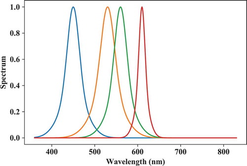
As a first example, let us start with the creation of four monochromatic LEDs and import the module into the global namespace for ease of use. The output is given in Fig. 9.

Fig. 9. Four monochromatic leds generated with spd_builder().

# Import module luxpy.spdbuild:

import luxpy.toolboxes.spdbuild as spb

# Set peak wavelengths:

peakwl = [450,530,560,610]

# Set Full-Width-Half-Maxima:

fwhm = [30,35,30,15]

S = spb.spd_builder(peakwl = peakwl,\

           fwhm = fwhm)

# Plot component spds:

lx.SPD(S).plot()

Next, let us create three additional spectra: two phosphor-type LED spectra (one with one phosphor and one with two phosphors) and one monochromatic LED-type spectrum (see Fig. 10 for output):

Fig. 10. Two phosphor-type and one monochromatic LED spectrum generated with spd_builder().

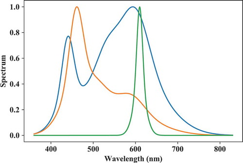
# peak wavelengths of monochromatic leds:

peakwl = [440,460,610]

# Full-Width-Half-Maximas:

fwhm = [30,35,15]

# Set phosphor strengths (i.e. alpha factor:

# in Smet et al. 2011):

strength_ph = [1.5, 0.4, 0]

# Set phosphor 1 parameters:

strength_ph1 = [1, 1, 0] # beta factor

peakwl_ph1 = [530, 510, 510]

fwhm_ph1 = [60, 60, 60]

# Set phosphor 2 parameters:

strength_ph2 = [2, 1, 0] # beta factor

peakwl_ph2 = [600, 590, 590]

fwhm_ph2 = [70, 70, 70]

S = spb.spd_builder(peakwl = peakwl,\

    fwhm = fwhm,\

    strength_ph = strength_ph, \

    strength_ph1 = strength_ph1,\

    peakwl_ph1 = peakwl_ph1,\

    fwhm_ph1 = fwhm_ph1,\

    strength_ph2 = strength_ph2,\

    peakwl_ph2 = peakwl_ph2,\

    fwhm_ph2 = fwhm_ph2)

# Plot component spds:

lx.SPD(S).plot()

One can also set them at a specific target chromaticity, specified by a “target” input argument (“tar_type ” specifies the type of target; for example, “cct”, “Yxy”, …, and “cspace_bwtf” is adict specifying the parameters need for the backward transformation called in colortf() inside spd_builder()). The code below calculates the fluxes required for a CCT = 3500 K (Duv = 0). There are only two spectra plotted in Fig. 11 as any set of three spectral components—that is, a monochromatic LED and two phosphors—for which the target is out of gamut results in an array of NaNs.

Fig. 11. Two phosphor-type LED spectra generated with spd_builder() for which the target chromaticity (CCT = 3500 K, Duv = 0) was inside the gamut spanned by its components.

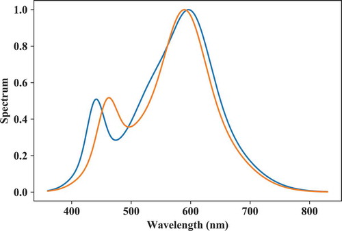
# CIE standard 2° observer:

cieobs = '1931_2'

cspace_bwtf = {'cieobs' : cieobs,\

        'mode' : 'search'}

S = spb.spd_builder(peakwl = peakwl,\

    fwhm = fwhm,\

    strength_ph = strength_ph,\

    strength_ph1 = strength_ph1,\

    peakwl_ph1 = peakwl_ph1,\

    fwhm_ph1 = fwhm_ph1,\

    strength_ph2 = strength_ph2,\

    peakwl_ph2 = peakwl_ph2,\

    fwhm_ph2 = fwhm_ph2,\

    target = 3500,\

    tar_type = 'cct',\

    cspace_bwtf = cspace_bwtf)

# Plot component spds:

lx.SPD(S).plot()

The package also supports spectra optimization beyond the target chromaticity when there are more than three spectral components provided.

The following code block provides a practical example of flux optimization with fixed component spectra using objective functions for a target CCT of 4000 K (Duv = 0). The objective functions and their target values are specified as two lists. For this example, the IES TM30 R_f and R_g color rendition measures (IES 2015) were chosen with target values of respectively 90 and 110. The output is plotted in Fig. 12. The optimization is done using the “2mixer” optimizer (another option is “3mixer”). For more information on the optimization algorithms, the reader is referred to the __doc__ string of the lx.spdbuild.spd_optimizer function.

Fig. 12. Spectrum optimized from predefined, fixed component spectra for a CCT = 3500 K and IES TM30 R_f and R_g objective functions.

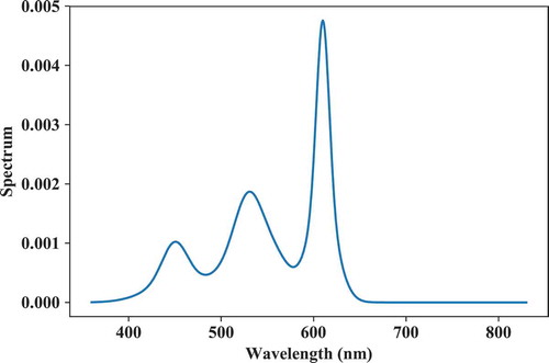
# Set target chromaticity:

target = 3500

# Set objective functions and targets:

obj_fcn = [lx.cri.spd_to_iesrf,\

      lx.cri.spd_to_iesrg]

obj_tar_vals = [90,110]

# Set component model parameters:

peakwl = [450,530,560,610]

fwhm = [30,35,30,15]

# Perform optimization:

S,_ = spb.spd_optimizer(target = target, \

     tar_type = 'cct',\

     cspace_bwtf = cspace_bwtf,\

     optimizer_type = '2mixer',\

     peakwl = peakwl,\

     fwhm = fwhm,\

     obj_fcn = obj_fcn,\

     obj_tar_vals = obj_tar_vals)

# Check output agrees with target:

xyz = lx.spd_to_xyz(S, relative = False,\

           cieobs = cieobs)

cct = lx.xyz_to_cct(xyz, cieobs = cieobs,\

        mode = 'search')[0,0]

Rf, Rg = [fcn(S)[0,0] for fcn in obj_fcn]

print('\nResults (optim,target):')

print(“cct(K): ({:1.1f},{:1.1f})”.format(cct, \ target))

print(“Rf: ({:1.2f},{:1.2f})”.format(Rf, \  obj_tar_vals[0]))

print(“Rg: ({:1.2f}, {:1.2f})”.format (Rg,  obj_tar_vals[1]))

#plot spd:

plt.figure()

lx.SPD(S).plot()

Output:

Optimization terminated success-fully.

Current function value: 0.077599

Iterations: 23

Function evaluations: 48

Results (optim,target):

cct(K): (3500.0,3500.0)

Rf: (85.98,90.00)

Rg: (103.02, 110.00)

In addition to lux-only optimization, the peak wavelengths and full-width half-maxima (FWHM) of the components can be optimized. The example below calculates a spectrum with a CCT of 3500 K (Duv = 0) and optimized for IES TM30 R_f and R_g target values of respectively 90 and 110. The spectrum is built from six components with free peak wavelength, FWHM, and fluxes. The verbosity argument toggles intermediate output of objective functions values on and off. The optimized spectrum is shown in Fig.13.

Fig. 13. Spectrum optimized from predefined, fixed component spectra for a CCT = 3500 K and IES TM30 R_f and R_g objective functions.

# Perform optimization:

S,_ = spb.spd_optimizer(target = target, \

    tar_type = 'cct',\

    cspace_bwtf = cspace_bwtf,\

    optimizer_type = '2mixer',\

    N_components = 6,\

    obj_fcn = obj_fcn,\

    obj_tar_vals = obj_tar_vals,\

    verbosity = 0)

# Check output agrees with target:

xyz = lx.spd_to_xyz(S, relative = False,\

            cieobs = cieobs)

cct = lx.xyz_to_cct(xyz, cieobs = cieobs,\

mode = 'search')[0,0]

Rf, Rg = [fcn(S)[0,0] for fcn in obj_fcn]

print('\nResults (optim,target):')

print(“cct(K):({:1.1f},{:1.1f})”.format(cct,\ target))

print(“Rf: ({:1.2f},{:1.2f})”.format(Rf, \  obj_tar_vals[0]))

print(“Rg: ({:1.2f}, {:1.2f})”. format(Rg,  obj_tar_vals[1]))

#plot spd:

plt.figure()

lx.SPD(S).plot()

Output:

Optimization terminated success-fully.

Current function value: 0.002494

Iterations: 1356

Function evaluations: 2037

Results (optim,target):

cct(K): (3500.0,3500.0)

Rf: (89.85,90.00)

Rg: (109.79, 110.00)

5.11. Simulation and Rendering of Hyperspectral Images (.hypspcim)

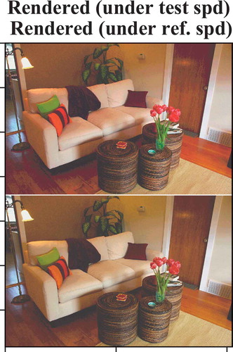
LuxPy contains a module that can simulate a hyperspectral image of any regular sRGB image by mapping the color coordinates of each pixel in the image to a sample from a spectral reflectance set that is near-metameric under CIE D65 or some other user-specified reference spectrum. The algorithm uses SciPy’s cKDTree to find the closest neighbors to each pixel’s color coordinates and then calculates a weighted mean of the nearest spectral reflectance functions in a set. The render_image function can then simulate the effect of a light source on the color appearance of the imaged scene to explore the source’s color rendition properties. Note though that no account is taken (yet) for out-of-gamut values (that is, no extrapolation has been implemented and out of gamut color coordinates are simply clipped). The user can provide a set of reflectance functions or the IESTM30 4880 reference set (IES 2015) is used as default. There is also the option to apply a von Kries chromatic adaptation to the reference spectrum chromaticity, whereby the user can specify the degree of adaptation by input argument D. The following illustrates the use of the render_image function:

from luxpy import hypspcim

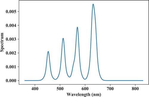
# Generate 4000 K RGB LED spectrum:

S=spb.spd_builder(peakwl = [450,530,610],\

        fwhm = [10,10,10],\

        target = 4000,\

        tar_type = 'cct')

# Specify filename (+path) to some image or

# read in ndarray with image data.

# In this case the filename of the default # image was used for simplicity:

img = hypspcim._HYPSPCIM_DEFAULT_IMAGE

# Calculate hyper-spectral version

# of the img image:

img_hyp = hypspcim.render_image(img = img,\

        cspace = 'ipt',\

        spd = S, \

        D = 1, \

        show = True,\

        stack_test_ref = 21)

print(img_hyp.shape)

Output:

(681, 1024, 401)

In the code above, the stack_test_ref argument specifies how the rendered images under the test and reference light sources should be stacked. The output of the rendering is shown in Fig. 14.

Fig. 14. Rendering results of simulated hyperspectral images. Top: using the 4000 K RGB LED test light source spectrum. Bottom: using the reference (D65) spectrum. A von Kries chromatic adaptation with degree of adaptation set to D = 1 has been applied.

6. Summary

This article described the installation of the LuxPy toolbox and provided an overview of its basic design and functionality. It also demonstrated its basic usage by providing several code examples using a Jupyter notebook. It is hoped that the LuxPy package—written in an easy-to-learn open-source programming language—would be useful to many lighting and color researchers and professionals and would stimulate collaborative research and ease sharing of calculations and analyses.

Disclosure statement

The author reports no declarations of interest.

Additional information

Funding

The author reports no funding for the preparation of this article.

References

- AS/NZS1680.2.5. 1997. INTERIOR LIGHTING PART 2.5: HOSPITAL AND MEDICAL TASKS. Homebrush (Australia): Standards.
- Asano Y, Fairchild MD, Blondé L. 2016. Individual colorimetric observer model. PLoS One. 11:1–19.
- CIE13.3-1995. 1995. Method of measuring and specifying colour rendering properties of light sources. Vienna (Austria): CIE.
- CIE15-2004. 2004. Colorimetry. Vienna (Austria): CIE.
- CIE224:2017. 2017. CIE 2017 colour fidelity index for accurate scientific use. Vienna (Austria): CIE.
- CIE-TN003:2015. 2015. Report on the first international workshop on circadian and neurophysiological photometry, 2013. Vienna (Austria): CIE.
- David A, Fini PT, Houser KW, Ohno Y, Royer MP, Smet KAG, Wei M, Whitehead L. 2015. Development of the IES method for evaluating the color rendition of light sources. Opt Express. 23:15888–15906.
- Davis W, Ohno Y. 2010. Color quality scale. Opt Eng. 49:33602–33616.
- IES. 2015. IES-TM-30-15: method for evaluating light source color rendition. New York (NY): The Illuminating Engineering Society of North America.
- Li C, Li Z, Wang Z, Xu Y, Luo MR, Cui G, Melgosa M, Brill MH, Pointer M. 2017. Comprehensive color solutions: CAM16, CAT16, and CAM16-UCS. Color Res Appl. 1–16.
- Lucas RJ, Peirson SN, Berson DM, Brown TM, Cooper HM, Czeisler CA, Figueiro MG, Gamlin PD, Lockley SW, O’Hagan JB, et al. 2014. Measuring and using light in the melanopsin age. Trends Neurosci. 37:1–9.
- Luo MR, Cui G, Li C. 2006. Uniform colour spaces based on CIECAM02 colour appearance model. Color Res Appl. 31:320–330.
- MathWorks Inc. 2018. Matlab. Natick (MA): Mathworks, Inc.
- Moroney N, Fairchild MD, Hunt RWG, Li C, Luo MR, Newman T. 2002. The CIECAM02 color appearance model. Scottsdale (AZ): IS&T/SID Tenth Color Imaging Conf. 10:23.
- Ohno Y. 2005. Spectral design considerations for white LED color rendering. Opt Eng. 44:111302.
- Ohno Y. 2014. Practical use and calculation of CCT and Duv. LEUKOS. 10:47–55.
- Rea MS, Figueiro MG, Bierman A, Hamner R. 2012. Modelling the spectral sensitivity of the human circadian system. Light Res Technol. 44:386–396.
- Sharma G, Wu W, Dalal EN. 2005. The CIEDE2000 color‐difference formula: implementation notes, supplementary test data, and mathematical observations. Color Res Appl. 30:21–30.
- Smet K, Ryckaert WR, Pointer MR, Deconinck G, Hanselaer P. 2011. Optimal colour quality of LED clusters based on memory colours. Opt Express. 19:6903–6912.
- Smet K, Schanda J, Whitehead L, Luo R. 2013. CRI2012: A proposal for updating the CIE colour rendering index. Light Res Technol. 45:689–709.
- Smet KAG, Ryckaert WR, Pointer MR, Deconinck G, Hanselaer P. 2012. A memory colour quality metric for white light sources. Energy Build. 49:216–225.
- Smet KAG, Webster MA, Whitehead LA. 2016. A simple principled approach for modeling and understanding uniform color metrics. J Opt Soc Am. 33:A319–A331.
- Smet KAG, Zhai Q, Luo MR, Hanselaer P. 2017. Study of chromatic adaptation using memory color matches, Part I: neutral illuminants. Opt Express. 25:7732–7748.
- Withouck M, Smet KAG, Ryckaert WR, Hanselaer P. 2015. Experimental driven modelling of the color appearance of unrelated self-luminous stimuli: CAM15u. Opt Express. 23:12045–12064.
- Document Foundation. 2018. LibreCalc.www.libreoffice.org.