Reconstruction of Daylight Spectral Power Distribution Based on Correlated Color Temperature: A Comparative Study between the CIE Approach and Localized Procedures in Assessing Non-image Forming Effects

ABSTRACT

Spectrally and spatially resolved information on daylight is critically important when planning for non-image forming (NIF) responses. Nevertheless, the availability of such data is scarce given the high initial costs and complex on-site maintenance of high-end spectral measurement devices. The CIE (Commission Internationale de l’Éclairage) reconstruction procedure allows for the derivation of the daylight spectral power distribution (SPD) from the chromaticity coordinates or the correlated color temperature ($T_{cp}$). However, several studies have suggested that both the daylight locus and the reconstruction procedure are erroneous, and specifically SPDs with a higher $T_{cp}$ cannot be reproduced accurately.

This paper studies the reconstruction accuracy of the SPD of daylight, and contextualizes the findings in relation to NIF effects. The analysis comprises a comparative study to determine the accuracy of the CIE procedure compared to two localized reconstruction procedures, and a sensitivity study to examine the impact of accuracy on the assessment of NIF responses, as represented by all five retinal photoreceptors and expressed in the α-opic efficacy of luminous radiation. The results indicated that a localized procedure, adjusting both the daylight locus and the PCA components of daylight, outperformed the CIE reconstruction method. However, improvement in the reconstruction accuracy had no effect on NIF assessment. The RSMPE for α-opic quantities did not exceed 4% for any procedure. In practical terms, this implies that cost-effective sensors and the representation of spectral properties in sky models with a single value – the correlated color temperature – can be used for NIF purposes. These findings bridge theory and practice by opening up new insights into the understanding of simplified methods used to determine NIF effects of daylight.

HIGHLIGHTS

• Using a localized procedure to define spectral power distribution (SPD) based on correlated color temperature ($T_{cp}$) outperforms the CIE method.

• Accuracy depends on the computation procedure rather than the daylight locus location.

• Higher accuracy does not affect the α-opic responses used in defining non-image forming (NIF) effects.

• Findings confirm the applicability of simplified measuring and representation methods for daylight SPDs.

• $T_{cp}$ can be used to represent daylight SPD in planning software to assess NIF effects.

KEYWORDS:

• Daylight
• reconstruction procedure
• spectral power distribution
• daylight locus
• non-image forming effects

1. Introduction

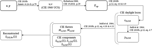
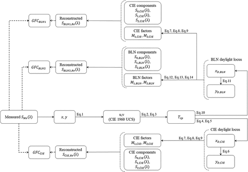
Understanding the spectral, spatial, and temporal variation in daylight is crucial when planning for spectrally selective responses to the light. Recent findings in the field of chronobiology on non-image forming effects have increased the need for accurate spectrally resolved information on daylight, especially because one subset of these responses, ipRGC-influenced light (IIL) responses, is primarily induced by light with a strong bluish component (Knoop et al. 2020; Münch et al. 2020). Precise spectral measurements, however, require advanced and thus rather expensive measuring equipment. Consequently, the amount of spectral data on daylight worldwide is limited. Data from several studies has suggested that the spectrum of daylight has a distinct profile (Condit and Grum 1964; Henderson and Hodgkiss 1963; Hernández-Andrés et al. 2001b; Judd et al. 1964; Kawakami et al. 1965; Knoop et al. 2015; Nayatani and Wyszecki 1963; Sastri and Das 1968; Sekine 1989, 1991; Tarrant 1968; Winch et al. 1966). In 1964, based on 622 spectral measurements, Judd et al. (1964) proposed a reconstruction procedure for spectral power distribution (SPD) of daylight. The procedure, later adopted by the Commission Internationale de l’Éclairage (CIE), enables the determination of the terrestrial daylight spectrum from either chromaticity coordinates ($x,y$) or correlated color temperature ($T_{cp})$ (CIE 2018b; Robertson 1968). For practical application, this means that daylight can be measured using cost-effective and widely accessible sensors (Hernández-Andrés et al. 2004). Applying this reconstruction procedure allows to derive the approximate SPD, which then can be weighted according to virtually any given action spectrum depending on the application. This presents, for example, the opportunity to measure light in daylight studies to determine non-image forming effects (Knoop et al. 2019a; Münch et al. 2020; Schlangen and Price 2021; Wirz-Justice et al. 2020), as well as the development of lighting control systems that can support these effects (Weber et al. 2016). Furthermore, the procedure makes it possible to display the color characteristics of daylight in planning software using a single value, its $T_{cp}$ (Diakite et al. 2018; Knoop et al. 2019b). This is used, for example, in spectral sky models (Chain 2004; Diakite-Kortlever and Knoop 2021; Rusnák 2014; Takagi et al. 1990). However, the CIE (2018b) explicitly noted the possible occurrence yet missing information on both seasonal and geographical variations in the SPD of daylight. Moreover, recent studies have suggested that both the daylight locus (Dixon 1978; Henderson 1977; Sastri and Das 1968; Sekine 1989, 1991; Winch et al. 1966) and the reconstruction procedure (Chain 2004; Diakite and Knoop 2019; Hernández-Andrés et al. 2001a, 2001b; Kobayashi et al. 1997, 1996) are hardly error-free, and that the daylight spectra for higher correlated color temperatures are especially difficult to reproduce accurately (Hernández-Andrés et al. 2001b; Rusnák 2014). Furthermore, as far as we are aware, no studies exist determining whether an increase in the accuracy of the reconstruction due to local adjustments would have a significant impact on the assessment of non-image forming (NIF) responses.

In order to characterize daylight and to assess its potential, for example to induce NIF effects, with a single-value representation or cost-effective and widely accessible sensors, this paper addresses the accuracy of the reconstruction procedure of daylight spectra as a function of $T_{cp}$. The aim of the work presented in this publication is threefold: (i) to review the CIE procedure for the reconstruction of the daylight spectrum, using long-term measurements from Berlin; (ii) to investigate the extent to which the accuracy of the reconstruction is improved when the procedure is adapted locally; and (iii) to verify whether higher accuracy in the reconstruction procedure due to local adaptation accounts for a relevant increase in the accuracy of the NIF assessment.

2. State of the art: approaches to the reconstruction of daylight spectral power distribution

A large body of evidence from experimental studies indicates that the SPD of daylight exhibits a distinctive profile (Condit and Grum 1964; Henderson and Hodgkiss 1963; Hernández-Andrés et al. 2001b; Judd et al. 1964; Kawakami et al. 1965; Knoop et al. 2015; Nayatani and Wyszecki 1963; Sastri and Das 1968; Sekine 1989, 1991; Tarrant 1968; Winch et al. 1966). Moreover, numerous studies have shown that daylight chromaticities can be represented with a curve that runs nearly parallel to the Planckian locus, called the daylight locus (CIE 2018b; Judd et al. 1964). Therefore, it is possible to not only assign a particular $T_{cp}$ to a specific daylight chromaticity coordinate ($x_D,y_D$) (Hernández-Andrés et al. 1999; McCamy 1992; Robertson 1968), but also a characteristic, distinctive, SPD (Condit and Grum 1964; Henderson and Hodgkiss 1963; Judd et al. 1964; Sastri and Das 1968). In 1964, in their landmark publication, Judd et al. (1964) subjected 622 daylight SPDs to principal component analysis (PCA) as described by Simonds (1963). PCA is a linear procedure to reduce the dimensionality of a set of responses to a low-dimensional space while retaining an intrinsic minimum that accounts for much of the variance in the original data set. Accordingly, Judd et al. (1964) determined three components that represented most of the variance of the composite data set, which allowed them to reconstruct the SPD for daylight at selected $T_{cp}$. The data subsets were compiled in three different locations (99 measured by Budde, unpublished, in Ottawa, CA; 249 by Condit and Grum (1964) in Rochester, USA; and 274 by Henderson and Hodgkiss (1963) in Enfield, UK) and differed in the number of measured spectra, the length of recording, and the choice of the measuring approach, including measuring equipment. Based on the composite data set, Judd et al. (1964) visually determined (Henderson 1977) a daylight locus of typical daylight chromaticities (hereafter referred to as the “CIE daylight locus”).

The reconstruction procedure was later adapted by the CIE (2018b) by making minor adjustments (interpolation to the 5 nm interval for a wavelength bandwidth between 300 nm and 830 nm) and then incorporating equations for conversion of $T_{cp}$ to the chromaticity $x_D$ in the range between 4000 K to 25,000 K into the procedure. These equations were first introduced by Wright (1965), then modified by the CIE Colorimetry Committee (described in Robertson (1968) and Henderson (1977, pp. 203–204), and later slightly altered in light of the revised value of Planck’s second radiation constant $c_2$ (described in Henderson (1977, pp. 316–317)). Additional groundbreaking research by Robertson (1968) presented a numerical interpolation method to compute the $T_{cp}$ from the SPD and thus from the $x,y$ of a light source, which further extended the reconstruction procedure by enabling the derivation of the SPD from chromaticities. Figure 1 summarizes the approach to reconstructing SPD using either $x,y,$ or $T_{cp}$.

Fig. 1. Schematic representation of the CIE (2018b) reconstruction procedure approach to reconstructing daylight spectral power distribution ($S\left(\lambda \right)$) as a function of either chromaticity coordinates ($x,y$) or correlated color temperature ($T_{cp}$).

The equations used to reconstruct the SPD of daylight as function of $x,y$ or $T_{cp}$ are shown in the step-by-step outline below.

If the $T_{cp}$ is not given, the CIE (2018b) recommended calculating it from the chromaticities $x,y$ according to Robertson (1968). For this, the chromaticity coordinates are first converted to the corresponding ($u,v$) in the CIE 1960 uniform chromaticity scale (USC) diagram as follows:

(1) $u=\frac{4x}{-2x+12y+3};v=\frac{6y}{-2x+12y+3}$(1)

The $T_{cp}$ can then be found by interpolation between the two closest isotemperature lines. Each line corresponds with a constant correlated color temperature $T_i$, and a certain slope ($m_i$). A set of 31 isotemperature lines with the values of $T_i$, $u_i,v_i$, and $m_i$ is tabulated in Robertson (1968, Table II). The $T_{cp}$ is calculated in two steps. First by calculating the distance ($d_i$) of the measured (test) chromaticity coordinate ($u_T,v_T$) from each line in the set of 31 isotemperature lines using Equation (2)(2) $d_i=\frac{\left[\left(v_T-v_i\right)-m_i\left(u_T-u_i\right)\right]}{{\left(1+m_i^2\right)}^{1/2}}$(2) (Robertson 1968, Equation 4). The measured chromaticities lie between two adjacent lines ($i=j$ and $i=j+1$) for which the term $\frac{d_j}{d_{j+1}}$ is negative. Second, by calculating the $T_{cp}$ according to Equation (3)(3) $T_{cp}={\left[\frac{1}{T_j}+\frac{d_j}{d_j-d_{j+1}}\left(\frac{1}{T_{j+1}}-\frac{1}{T_j}\right)\right]}^{-1}$(3) (Robertson 1968, Equation 5b):

(2) $d_i=\frac{\left[\left(v_T-v_i\right)-m_i\left(u_T-u_i\right)\right]}{{\left(1+m_i^2\right)}^{1/2}}$(2)

(3) $T_{cp}={\left[\frac{1}{T_j}+\frac{d_j}{d_j-d_{j+1}}\left(\frac{1}{T_{j+1}}-\frac{1}{T_j}\right)\right]}^{-1}$(3)

Table 1. Compilation of the reconstruction methods of daylight

Publication	Location(s)	Measuring procedure	Length of record	Number of SPDs	Daylight locus	$S_i\left(\lambda \right)$^a with $\left|i\right|$ equal
Judd et al. (1964) CIE (2018b)	Ottawa, Canada ^Budde, unpublished (Henderson 1977)	Daylight and skylight, northern sky (global spectral irradiance)	Mar – Apr 1963	99	y = −3.000x^2+ 2.870x – 0.275	3
	Rochester, USA ^Condit and Grum (1964)	Daylight (global spectral irradiance)	Jun-Jul 1962	249
	Enfield, UK ^Henderson and Hodgkiss (1963)	Daylight and skylight, northern sky (global spectral irradiance)	Apr 1961 – Mar 1962	274
Sastri and Das (1968)	New Delhi, India	Skylight, northern sky (global spectral irradiance)	1964– 1965	187	n/a	3
Dixon (1978)	Coburg, Australia	Daylight (global spectral irradiance)	Sep 1975 – Mar 1976	113	y = 2,2210x^2 − 0.4888x + 0.2553	5
	Bendigo, Australia	Skylight (global spectral irradiance)	Oct 1976	123	y = −0.96000x^2+ 1.58500x – 0.08054	4
Kobayashi et al. (1996)	Atsugi, Japan	Skylight, northern sky (spectral irradiance E(e, λ, 45°)	Jan -Mar 1991	220	y = −1.8500x^2+ 2.1010x – 0.1520	3
Kobayashi et al. (1997)	Nagaoka, Japan	Skylight, northern sky (spectral irradiance E(e, λ, 35, 55°)	Nov 1990 – Dec 1996	847	y = −1.469x^2+ 1.887x – 0.120	3
Hernández-Andrés et al. (2001a)	Granada, Spain	Skylight (spectral irradiance E(e, λ, 3°)	Feb – Aug 1998	1567	y = −2.77935x^2+ 2.72203x – 0.24770	3 or 6
Hernández-Andrés et al. (2001b)	Granada, Spain	Daylight (global spectral irradiance on horizontal plane)	Feb 1996 – Feb 1998	2600	y = −1.09234x^2+ 1.55320x – 0.05188	3 or 6
Chain (2004)	Vaulx-en-Velin, France	Skylight: diffuse, spectral irradiance E(e, λ, 1°)	n/a	7732	y = −3.2877x^2+ 2.9668x – 0.27683	3 or 5
	Vaulx-en-Velin, France	Skylight: diffuse, spectral irradiance E(e, λ, 1°)	n/a	7732	y = 781.4x^4– 910.05x^3+ 391.62x^2– 72.718x + 5.1294	3 or 5
Rusnák (2014)	Bratislava, Slovakia	Skylight: diffuse, spectral irradiance E(e, λ, 11°)	2013	12,905	y = −2.576x^2+ 2.401x −0.166	3
	Bratislava, Slovakia	Global spectral irradiance	2013	89	y = −2.220x^2+ 2.166x – 0.132	3
Diakite et al. (2018)	Berlin, Germany	Skylight: diffuse, spectral irradiance E(e, λ, 10°)	Jan – Dec 2016 for modeling and Jan – Dec 2015 for validation	23,085 (2016) and 22,419 (2015)	y = −1.2848x^2+ 1.7519x – 0.0937	3

^a$S_i\left(\lambda \right)$: components, functions of wavelength,$\lambda$

Table 2. Summary of the CIE and locally adjusted reconstruction approaches

	CIE	BLN1	BLN2
$x_D$	$x_{D,CIE}$ from CIE (2018b), Equations(4) $x_{D,CIE}=\frac{-4,6070\cdot {10}^9}{{T_{cp}}^3}+\frac{2,9678\cdot {10}^6}{{T_{cp}}^2}+\frac{0,09911\cdot {10}^3}{T_{cp}}+0,244063$(4) (4(4) $x_{D,CIE}=\frac{-4,6070\cdot {10}^9}{{T_{cp}}^3}+\frac{2,9678\cdot {10}^6}{{T_{cp}}^2}+\frac{0,09911\cdot {10}^3}{T_{cp}}+0,244063$(4) ) and (5(5) $x_{D,CIE}=\frac{-2,0064\cdot {10}^9}{{T_{cp}}^3}+\frac{1,9018\cdot {10}^6}{{T_{cp}}^2}+\frac{0,24748\cdot {10}^3}{T_{cp}}+0,237040$(5) )	$x_{D,BLN}$ from Equation(10) $x_{D,BLN}=\frac{-4.5036\cdot {10}^9}{{T_{cp}}^3}+\frac{2.5225\cdot {10}^6}{{T_{cp}}^2}+\frac{0.22336\cdot {10}^3}{T_{cp}}+0.23535$(10) (10(10) $x_{D,BLN}=\frac{-4.5036\cdot {10}^9}{{T_{cp}}^3}+\frac{2.5225\cdot {10}^6}{{T_{cp}}^2}+\frac{0.22336\cdot {10}^3}{T_{cp}}+0.23535$(10) )	$x_{D,BLN}$ from Equation(10) $x_{D,BLN}=\frac{-4.5036\cdot {10}^9}{{T_{cp}}^3}+\frac{2.5225\cdot {10}^6}{{T_{cp}}^2}+\frac{0.22336\cdot {10}^3}{T_{cp}}+0.23535$(10) (10(10) $x_{D,BLN}=\frac{-4.5036\cdot {10}^9}{{T_{cp}}^3}+\frac{2.5225\cdot {10}^6}{{T_{cp}}^2}+\frac{0.22336\cdot {10}^3}{T_{cp}}+0.23535$(10) )
Daylight locus $y_D$	$y_{D,CIE}$ from CIE (2018b), Equation(6) $y_{D,CIE}=-3.000\cdot {x_D}^2+2.870\cdot x_D-0.275$(6) (6(6) $y_{D,CIE}=-3.000\cdot {x_D}^2+2.870\cdot x_D-0.275$(6) )	$y_{D,BLN}$ from Equation(11) ${\mathrm{y}}_{\mathrm{D},\mathrm{B}\mathrm{L}\mathrm{N}}=-2.0795x_{\mathrm{D},\mathrm{B}\mathrm{L}\mathrm{N}}^2+2.2376x_{\mathrm{D},\mathrm{B}\mathrm{L}\mathrm{N}}-0.16974$(11) (11(11) ${\mathrm{y}}_{\mathrm{D},\mathrm{B}\mathrm{L}\mathrm{N}}=-2.0795x_{\mathrm{D},\mathrm{B}\mathrm{L}\mathrm{N}}^2+2.2376x_{\mathrm{D},\mathrm{B}\mathrm{L}\mathrm{N}}-0.16974$(11) )	$y_{D,BLN}$ from Equation(11) ${\mathrm{y}}_{\mathrm{D},\mathrm{B}\mathrm{L}\mathrm{N}}=-2.0795x_{\mathrm{D},\mathrm{B}\mathrm{L}\mathrm{N}}^2+2.2376x_{\mathrm{D},\mathrm{B}\mathrm{L}\mathrm{N}}-0.16974$(11) (11(11) ${\mathrm{y}}_{\mathrm{D},\mathrm{B}\mathrm{L}\mathrm{N}}=-2.0795x_{\mathrm{D},\mathrm{B}\mathrm{L}\mathrm{N}}^2+2.2376x_{\mathrm{D},\mathrm{B}\mathrm{L}\mathrm{N}}-0.16974$(11) )
Components $S_0$, $S_1$, $S_2$	$S_{0,CIE}$, $S_{1,CIE}$, $S_{2,CIE}$ from CIE (2018b), Equation(7) $S_{CIE}\left(\lambda \right)=S_{0,CIE}\left(\lambda \right)+M_{1,CIE}\cdot S_{1,CIE}\left(\lambda \right)+M_{2,CIE}\cdot S_{2,CIE}\left(\lambda \right)$(7) (7(7) $S_{CIE}\left(\lambda \right)=S_{0,CIE}\left(\lambda \right)+M_{1,CIE}\cdot S_{1,CIE}\left(\lambda \right)+M_{2,CIE}\cdot S_{2,CIE}\left(\lambda \right)$(7) )	$S_{0,CIE}$, $S_{1,CIE}$, $S_{2,CIE}$ from CIE (2018b), Equation(7) $S_{CIE}\left(\lambda \right)=S_{0,CIE}\left(\lambda \right)+M_{1,CIE}\cdot S_{1,CIE}\left(\lambda \right)+M_{2,CIE}\cdot S_{2,CIE}\left(\lambda \right)$(7) (7(7) $S_{CIE}\left(\lambda \right)=S_{0,CIE}\left(\lambda \right)+M_{1,CIE}\cdot S_{1,CIE}\left(\lambda \right)+M_{2,CIE}\cdot S_{2,CIE}\left(\lambda \right)$(7) )	$S_{0,BLN}$, $S_{1,BLN}$, $S_{2,BLN}$ from Equation(12) $S_{BLN}\left(\lambda \right)=S_{0,BLN}\left(\lambda \right)+M_{1,BLN}\cdot S_{1,BLN}\left(\lambda \right)+M_{2,BLN}\cdot S_{2,BLN}\left(\lambda \right)$(12) (12(11) ${\mathrm{y}}_{\mathrm{D},\mathrm{B}\mathrm{L}\mathrm{N}}=-2.0795x_{\mathrm{D},\mathrm{B}\mathrm{L}\mathrm{N}}^2+2.2376x_{\mathrm{D},\mathrm{B}\mathrm{L}\mathrm{N}}-0.16974$(11) )
Factors $M_1$ and $M_2$	$M_{1,CIE}$ and $M_{2,CIE}$ from CIE (2018b), Equations(8) $M_{1,CIE}=\frac{-1,3515-1,7703x_D+5,9114y_D}{0,0241+0,2562x_D-0,7341y_D}$(8) (8(8) $M_{1,CIE}=\frac{-1,3515-1,7703x_D+5,9114y_D}{0,0241+0,2562x_D-0,7341y_D}$(8) and 9(9) $M_{2,CIE}=\frac{0,0300-31,4424x_D+30,0717y_D}{0,0241+0,2562x_D-0,7341y_D}$(9) )	$M_{1,CIE}$ and $M_{2,CIE}$ from CIE (2018b), Equations(8) $M_{1,CIE}=\frac{-1,3515-1,7703x_D+5,9114y_D}{0,0241+0,2562x_D-0,7341y_D}$(8) (8(8) $M_{1,CIE}=\frac{-1,3515-1,7703x_D+5,9114y_D}{0,0241+0,2562x_D-0,7341y_D}$(8) and 9(9) $M_{2,CIE}=\frac{0,0300-31,4424x_D+30,0717y_D}{0,0241+0,2562x_D-0,7341y_D}$(9) )	$M_{1,BLN}$ and $M_{2,BLN}$ from Equations$M_{1,BLN}=\frac{5.0767-13.8483\cdot x_D-1.9943\cdot y_D}{0.0157+0.0469\cdot x_D-0.3791\cdot y_D}(13)$ (13$M_{1,BLN}=\frac{5.0767-13.8483\cdot x_D-1.9943\cdot y_D}{0.0157+0.0469\cdot x_D-0.3791\cdot y_D}(13)$ and 14$M_{2,BLN}=\frac{1.3617+61.3011\cdot x_D-62.6447\cdot y_D}{0.0157+0.0469\cdot x_D-0.3791\cdot y_D}(14)$)

In the following step, or if the $T_{cp}$ is given, the chromaticity coordinate of daylight $x_D$ along the CIE daylight locus is calculated as a function of $T_{cp}$ according to Equations(4) $x_{D,CIE}=\frac{-4,6070\cdot {10}^9}{{T_{cp}}^3}+\frac{2,9678\cdot {10}^6}{{T_{cp}}^2}+\frac{0,09911\cdot {10}^3}{T_{cp}}+0,244063$(4) (4(4) $x_{D,CIE}=\frac{-4,6070\cdot {10}^9}{{T_{cp}}^3}+\frac{2,9678\cdot {10}^6}{{T_{cp}}^2}+\frac{0,09911\cdot {10}^3}{T_{cp}}+0,244063$(4) and 5(5) $x_{D,CIE}=\frac{-2,0064\cdot {10}^9}{{T_{cp}}^3}+\frac{1,9018\cdot {10}^6}{{T_{cp}}^2}+\frac{0,24748\cdot {10}^3}{T_{cp}}+0,237040$(5) ) (CIE , 2018b, Equations 4.8 and 4.9), $x_D$ being within the range of 0.250 to 0.380, while bearing in mind a distinction in the calculation process for the two $T_{cp}$ regions: $4000\mathrm{K}<T_{cp}\le 7000\mathrm{K}$ and $7000\mathrm{K}<T_{cp}<25,000\mathrm{K}$.

For $4000\mathrm{K}<T_{cp}\le 7000\mathrm{K}$:

(4) $x_{D,CIE}=\frac{-4,6070\cdot {10}^9}{{T_{cp}}^3}+\frac{2,9678\cdot {10}^6}{{T_{cp}}^2}+\frac{0,09911\cdot {10}^3}{T_{cp}}+0,244063$(4)

For $7000\mathrm{K}<T_{cp}<25,000\mathrm{K}$:

(5) $x_{D,CIE}=\frac{-2,0064\cdot {10}^9}{{T_{cp}}^3}+\frac{1,9018\cdot {10}^6}{{T_{cp}}^2}+\frac{0,24748\cdot {10}^3}{T_{cp}}+0,237040$(5)

The chromaticity coordinate of daylight $y_D$ is found by the CIE daylight locus (CIE 2018b, Equation 4.7), given by:

(6) $y_{D,CIE}=-3.000\cdot {x_D}^2+2.870\cdot x_D-0.275$(6)

$x_D,y_D$ are used to define factors $M_1$ and $M_2,$which are then used to derive the relative SPD (CIE 2018b, Equation 4.10):

(7) $S_{CIE}\left(\lambda \right)=S_{0,CIE}\left(\lambda \right)+M_{1,CIE}\cdot S_{1,CIE}\left(\lambda \right)+M_{2,CIE}\cdot S_{2,CIE}\left(\lambda \right)$(7)

where $S_0\left(\lambda \right)$, $S_1\left(\lambda \right)$, and $S_2\left(\lambda \right)$ are components, functions of wavelength ($\lambda$), as tabulated in CIE (2018b, pp. 54–55, Table 6).

Table 3. Percentage of colorimetrically “accurate” ($GFC\ge 0.9950$), “good” ($GFC\ge 0.9990$), and “exact” ($GFC\ge 0.9999$) reconstructions depending on the reconstruction method

Classification	$GFC$	CIE	BLN1	BLN2
Accurate	$GFC\ge 0.9950$	95.97%	96.44%	99.72%
Good	$GFC\ge 0.9990$	0.004%	0.01%	67.74%
Exact	$GFC\ge 0.9999$	-	-	2.58%

Table 4. $\mathrm{M}\mathrm{e}\mathrm{a}\mathrm{n}\left(\mathrm{G}\mathrm{F}\mathrm{C}\right)$ values for three wavelength ranges and the complete wavelength range depending on the selected reconstruction method, color coded as follows: $GFC<0.9950$, $GFC\ge 0.9950$, $GFC\ge 0.9990$, $GFC\ge 0.9999$

Wavelength range	CIE method	BLN1 method	BLN2 method
$380nm\le \lambda \le 780nm$	0.99699	0.99714	0.99911
$380nm\le \lambda \le 490nm$	0.99806	0.99812	0.99975
$490nm<\lambda \le 585nm$	0.99970	0.99972	0.99988
$585nm<\lambda \le 780nm$	0.99389	0.99411	0.99780

Table 5. Mean (GFC) for sky conditions

Sky condition	CIE method	BLN1 method	BLN2 method
Overcast sky	0.99676	0.99692	0.99918
Intermediate sky	0.99708	0.99721	0.99915
Clear sky	0.99733	0.99743	0.99899

Table 6. $\mathrm{M}\mathrm{e}\mathrm{a}\mathrm{n}\left(\mathrm{G}\mathrm{F}\mathrm{C}\right)$ for summer and winter measurements

Season	CIE method	BLN1 method	BLN2 method
Summer (Jun, Jul, Aug)	0.99675	0.99689	0.99910
Winter (Dec, Jan, Feb)	0.99703	0.99726	0.99864

Where the factors $M_1$ and $M_2$ corresponding to the relevant eigenvectors are determined respectively based on the subsequent Equations(8) $M_{1,CIE}=\frac{-1,3515-1,7703x_D+5,9114y_D}{0,0241+0,2562x_D-0,7341y_D}$(8) (8(8) $M_{1,CIE}=\frac{-1,3515-1,7703x_D+5,9114y_D}{0,0241+0,2562x_D-0,7341y_D}$(8) and 9(9) $M_{2,CIE}=\frac{0,0300-31,4424x_D+30,0717y_D}{0,0241+0,2562x_D-0,7341y_D}$(9) ) (CIE 2018b, Equation 4.11)

(8) $M_{1,CIE}=\frac{-1,3515-1,7703x_D+5,9114y_D}{0,0241+0,2562x_D-0,7341y_D}$(8)

(9) $M_{2,CIE}=\frac{0,0300-31,4424x_D+30,0717y_D}{0,0241+0,2562x_D-0,7341y_D}$(9)

The CIE reconstruction procedure is widely used, but nevertheless, a number of studies have produced results that deviate considerably from the CIE reconstruction procedure (Chain 2004; Diakite et al. 2018; Dixon 1978; Hernández-Andrés et al. 2001a, 2001b; Kobayashi et al. 1997, 1996; Rusnák 2014; Sastri and Das 1968). Differences might occur due to the aforementioned existence of seasonal and geographical variations, acknowledged in the CIE (2018b), which might alter the SPD. Several studies (Chain 2004; Diakite et al. 2018; Dixon 1978; Henderson 1977; Hernández-Andrés et al. 2001a, 2001b; Kobayashi et al. 1997, 1996; Rusnák 2014; Sastri and Das 1968), especially those conducted in the southern hemisphere (Winch et al. 1966), have also reported considerable deviation from the CIE daylight locus, which as part of the procedure subsequently affects the accuracy of the reconstruction overall. More particularly, it has been found that the local daylight loci diverge from the CIE daylight locus in higher $T_{cp}$ (Diakite et al. 2018; Hernández-Andrés et al. 2001b). Other studies have noted inaccuracies at both ends of the visible spectrum (Chain 2004; Kobayashi et al. 1997). In particular, there have been inconsistencies in short wavelengths for high $T_{cp}$ (Kobayashi et al. 1997), which might be relevant for certain applications, e.g. the assessment of NIF effects. To improve on the existing CIE approach, Henderson (1977) called for a homogeneous data set based on measurements which relate to a single location and are subject to a systematized measuring process. This position has been endorsed by other researchers, whose work is presented below.

In this context, Hernández-Andrés et al. (1998) verified the procedure recommended by the CIE (based on the 622 SPD measurements from Judd et al. (1964)) using 252 daylight SPD measurements recorded in Granada, Spain. In addition to the CIE procedure, the accuracy of three other reconstruction procedures have been validated. Sastri and Das (1968) introduced the first, published in 1968, based on a data set of 187 SPD measurements of daylight taken in Delhi, India. The remaining two were carried out by Dixon (1978), published in 1978; these used two data sets, one developed from 113 SPD measurements conducted in an urban setting (Coburg, Australia), and the other drew on 123 SPD measurements gathered in the countryside, in Bendigo, Australia. Hernández-Andrés et al. (1998) used the average Goodness-of-Fit Coefficient ($\mathrm{G}\mathrm{F}\mathrm{C}$) to examine the reconstruction quality of the four reconstruction procedures, postulating that a $GFC\ge 0.9950$ represented a colorimetrically “accurate” reconstruction, a $GFC\ge 0.9990$ a “good” reconstruction, and a $GFC\ge 0.9999$ an “exact” reconstruction (Hernández-Andrés et al. 2001a, 2001b; Romero et al. 1997). Hernández-Andrés et al. (1998) concluded that, although the CIE procedure for the reconstruction method using chromaticity coordinates at the spectral range of 300 nm to 780 nm yielded the best average $GFC$ (at 5 nm, the average $GFC$ equaled 0.99505), no reconstruction was classified as “good” ($GFC\ge 0.9990$). Other relevant findings that emerged from the study were that finer resolution (5 nm as opposed to 10 nm) improved the quality of the reconstruction, and that more than four components were needed for spectrally accurate reconstruction. The latter finding was later reinforced by two follow-up studies. In 2001, Hernández-Andrés et al. (2001a, 2001b) modified the CIE reconstruction procedures and proposed two locally adjusted methods that incorporated daylight loci and components for Granada. The first was based on 1567 skylight measurements (with an aperture angle of 3°) from 44 measurement points, whereby the measuring point at zenith was measured four times per measurement series (Hernández-Andrés et al. 2001a). The $T_{cp}$ range was expanded, to range from 3804 K to higher than 10⁵ K. The second method was derived from 2600 daylight measurements (global spectral irradiance) with a $T_{cp}$ range between 3758 K and 34,573 K (Hernández-Andrés et al. 2001b). Hernández-Andrés et al. (2001a, 2001b) concluded that three components were sufficient for a colorimetrically and photometrically “accurate” ($GFC\ge 0.9950$) reconstruction; however, an almost exact ($GFC\ge 0.9999$) spectral fit in the visible area would require at least six components. The authors argued in favor of increased use of locally adapted loci representing different sites, rather than a generic locus used worldwide.

By Kobayashi et al. (1996, 1997) were unable to identify any major differences between locally adjusted approaches and the CIE approach from studies conducted in Japan in the wavelength range between 380 nm and 780 nm. They carried out a local adaptation of the reconstruction procedure and presented two daylight loci for two sites in Japan: Atsuki (based on 220 northern skylight measurements with an aperture angle of 0.48 sr) and Nagaoka (based on 847 northern skylight measurements with an aperture angle of 0.3 sr). The daylight loci did not show much difference from the CIE daylight locus, which might be attributed to limiting the considered chromaticity values to a maximum deviation of ±0.0003 from the CIE daylight locus in the u, v CIE chromaticity diagram. The authors found that, although there were discrepancies at both ends of the reconstructed spectrum, the approximation of the SPD with the CIE procedure in the, for human eye, visible wavelength range is very high, with an error of less than 1% (Kobayashi and Ikemori 1993). Therefore, the main goal of improving the method was to increase the accuracy of the reconstruction in the UV range. Kobayashi et al. (1997) noted, however, that the accuracy of the reconstructed SPD tended to decrease not only in the UV range, but also in the short wavelength range of light as $T_{cp}$ values continued to increase. The authors remarked that validation of the method for other sites is needed.

Similarly, Chain (2004) drew on the CIE (2018b) method to analyze 7732 spatially resolved skylight measurements gathered in Vaulx-en-Velin, France, with an aperture angle of 1°. Only measurements with no direct sunlight for solar altitudes ${\gamma }_S$ greater than 10° and $T_{cp}$ values higher than 4000 K were taken into consideration. Chain (2004) developed two locally adjusted functions describing the daylight chromaticity $x_D$ for two $T_{cp}$ categories in line with the CIE (2018b) procedure, and proposed two daylight loci, described by polynomials of the second and the fourth degree, respectively. Chain (2004) found that the resulting $T_{cp}$ yielded higher errors than when using the CIE functions, even for $T_{cp}$ greater than 100,000 K. Consequently, he retained the CIE coordinated chromaticity $x_D$ functions and the CIE daylight locus for the next stage of analysis. Next, Chain investigated local adjustment of the components $S_i\left(\lambda \right)$ and their corresponding factors $M_i$ at the spectral range of 380 nm – 780 nm. He then colorimetrically compared the two reconstruction methods, the CIE and the locally adapted one, reflected in color difference $\mathrm{\Delta }\mathrm{E}$. The CIE procedure yielded higher errors for high $T_{cp}$ on both sides of the visible spectrum. Nevertheless, the overall differences between the two methods were negligible, with the proposed method slightly outperforming the CIE method. However, given that the sampling data underlying both the modeling and the validation of the new procedure was the same since the differences in the output generated by the two methods were marginal, Chain opted against local adjustments, and thus for the retention of the CIE procedure for future analyses.

In order to modify and complement the existing CIE approach, in 2014, Rusnák (2014) derived two daylight loci from global measurements (89) and narrow-field measurements with an aperture angle of 11° (12,905) for Bratislava. The Bratislava daylight loci differed from the CIE daylight locus and were above the CIE daylight locus at high correlated color temperatures and below the CIE daylight locus at low correlated color temperatures. No comparison of methods was performed.

In a previous study (Diakite et al. 2018), we also evaluated the CIE procedure and developed a locally adapted preliminary procedure using a large database. To do so, we compiled two data sets from measurements gathered using a spectral sky scanner with an aperture angle of 10° at the Berlin Daylight Measuring Site in the city center of Berlin. The timeframe for modeling the Berlin daylight locus as well as for determining the local components covered the year 2016. A second data set, with measurements from 2015, was used to validate both the CIE procedure and the locally fitted model. The selected measurements with a spectral range of 380 nm – 780 nm were taken from sunrise to sunset at the full hour for ${\gamma }_S$ greater than 5°, for nine predefined sky areas that were never exposed to direct solar radiation at any point in the year, regardless of the sun’s position (oriented to the north, north-west, and north-east). This resulted in 2565 scans with 23,085 SPD measurements from 2016 to build the model, and 2559 scans with 22,419 SPD measurements from 2015 to validate it. Our study used the $GFC$ method with the classification proposed by Hernández-Andrés et al. (2001a, 2001b) to determine the accuracy of the SPD reconstructions using the CIE (2018b) procedure as well as the one adapted for Berlin. The accuracy of the reconstructions was evaluated as a function of the wavelength range, the $T_{cp}$, and the sky conditions.

Our analysis showed that reconstruction using the CIE method is possible, with 50% of the reconstructed SPD measurements qualifying as “accurate” ($GFC\ge 0.9950$); nevertheless, no “good” ($GFC\ge 0.9990$) or “exact” ($GFC\ge 0.9999$) reconstructions were achieved. On average, the reconstructions using the CIE method with $\mathrm{m}\mathrm{e}\mathrm{a}\mathrm{n}\left(\mathrm{G}\mathrm{F}{\mathrm{C}}_{\mathrm{C}\mathrm{I}\mathrm{E}}\right)=0.9942$ were below the threshold for a colorimetrically accurate reconstruction ($GFC\ge 0.9950$). Subsequent visual assessment indicated that the peaks were insufficiently mapped when using the resolution laid out by the CIE method (step size 5 nm). The locally adjusted procedure (step size 1 nm) yielded better results. A significantly higher $\mathrm{m}\mathrm{e}\mathrm{a}\mathrm{n}\left(\mathrm{G}\mathrm{F}{\mathrm{C}}_{\mathrm{B}\mathrm{L}\mathrm{N}}\right)=0.9970$ was achieved using the adjusted reconstruction procedure. Also, a greater number of “accurate” (60%), “good” (21%), and “exact” (0.02%) reconstructions were obtained using the localized procedure. The $\mathrm{m}\mathrm{e}\mathrm{a}\mathrm{n}\left(\mathrm{G}\mathrm{F}\mathrm{C}\right)$ was found to be at least colorimetrically “accurate” for all wavelength ranges of light (classified according to Rossotti (1983)), whereas reconstructions using the CIE method for wavelengths greater than 585 nm were on average colorimetrically inaccurate ($GFC<0.9950$). Visual assessment indicated that the replication of the peaks was more accurate in the reconstruction of the SPD with the localized procedure. High $T_{cp}$ values (approximately higher 7000 K) in particular were associated with the preliminary Berlin daylight locus deviating from the CIE daylight locus; this is consistent with previous observations, predominantly in Europe (Chain 2004; Hernández-Andrés et al. 2001a, 2001b). Such deviations may also explain the poorer accuracy of the reconstruction of clear skies observed by Yatsuzuka and Uetani (2014). In conclusion, using a locally adapted procedure reproduces more spectra for different sky conditions more effectively. However, the optimized procedure was limited to sky areas oriented to the north, and therefore the model was extended by all measured orientations.

Table 1 provides an overview of the above-mentioned approaches to reconstructing daylight spectra.

2.1. Problem statement

Dimension reduction and the resulting ease of use are the greatest advantages of the CIE reconstruction procedure. However, one principal limitation that several authors have noted is the sampling data underlying the method (Chain 2004; Henderson 1977; Hernández-Andrés et al. 2001a, 2001b; Kobayashi et al. 1997, 1996). The excessively short time period in which parts of the measurements for the analysis were carried out (the measurements in the USA (Condit and Grum 1964) only lasted four weeks) are the main reason why not all sky and weather conditions caused by seasonal variations are reflected in the data set. Location selection bias, which resulted in a model trained on a geographically biased data set (Kobayashi and Ikemori 1993) representing temperate climates occurring in middle latitudes in the northern hemisphere (specifically in Europe (Enfield, UK: 51°39ʹ N, 0°5ʹ W) and North America (Ottawa, ON, CA: 45°25ʹ N, 75°42′ W; Rochester, NY, USA: 44°0ʹ N, 123°6′ W)), is another potential concern for the possible underrepresentation of certain geographical and climatic variations. Another weakness of the data sets used by Judd et al. (1964) results from the differences in measurement approaches on which the data sets are based. The predominantly integral measurements result in an upper $T_{cp}$ limit of 25,000 K, which hinders an accurate representation of skylight with higher $T_{cp}$, typically from areas opposite of the sun under clear sky conditions (Diakite et al. 2018; Yatsuzuka and Uetani 2014). The extension of the bandwidth to 300 nm – 830 nm by extrapolation and the interpolated resolution of 5 nm used in the CIE procedure do not represent actual experimental results. Ultimately, using a visually determined daylight locus is one of the biggest weaknesses for a generally adopted procedure. A statistical fitting of the experimental chromaticities used in Judd et al. (1964) was later conducted by Nimeroff (Henderson 1977, p. 208), who found that the daylight locus in particular differed at high $T_{cp}$ values from the one proposed by Judd et al. (1964). Lastly, two different fittings for $x_D\left(T_{cp}\right)$ introduced a discontinuity in the data at 7000 K, which is permissible from a methodological viewpoint, but is undesirable in practical applications – i.e. simulation software. The procedure was mainly designed for colorimetric use, with the CIE stating that the extrapolated values accounted for “accurate enough” reconstruction for colorimetric purposes, but should not be used for other purposes. Consequently, the number of PCA components applied in the model served to reproduce daylight spectra satisfactorily from a colorimetric point of view; however, many other applications, in particular for spectral use, require higher resolution (1 nm). Older studies lacked today’s effective measuring instruments. Advances in technology and the increase in computing capacity have since enabled the recording and processing of these large amounts of data (Chain 2004; Inanici 2019; Knoop et al. 2015; Nieves et al. 2005; Riechelmann et al. 2013; Rusnák 2014; Tohsing et al. 2014; Yatsuzuka and Uetani 2013).

More recent studies have put the CIE procedure to the test with newer, larger, homogeneous data sets for single locations. In summary, the literature review showed that both the daylight locus and the reconstruction procedure seem site-dependent. This argues for changing to locally adapted daylight loci, as Henderson (1977) pointed out. Nonetheless, there is no consensus whether locally adjusting for different locations rather than using the CIE method universally would be more likely to result in better reconstructions and whether the differences in the accuracy of the reconstruction would be significant in relation to a given application. Another major drawback of the majority of the studies is validation, with the same data set as the one used for modeling. Most of the locally adapted procedures (except for the Dixon, and Sastri and Das procedures in Hernández-Andrés et al. (1998)) were not validated against data sets from other sites. For some studies, the measurement data are no longer available; other studies were only published in the native language; in many, the information underlying the results is not well documented, i.e., $S_i\left(\lambda \right)$, or $x_D$ and $y_D$ are graphically represented, but not actually tabulated. Further, the SPD is reproduced solely by means of the $T_{cp}$ or $x$and $y$, so the question arises of whether these parameters alone are sufficient for an accurate reconstruction, or whether other influencing factors should be identified, such as sky conditions, solar altitude, or atmospheric influences (Chain 2004). In reviewing the literature, no data was found on the association between the accuracy of the reconstruction and those above-mentioned factors. Furthermore, to the best of our knowledge, no previous studies have contextualized the significance of their method in relation to daytime NIF responses of daylight encompassing all five photoreceptors. In practical terms, this means that it is still unclear whether a reliable estimate of NIF responses, using any of the currently available reconstruction procedures, can be derived from either simplified measurements using inexpensive color sensors or $T_{cp}$ values from spectral sky models.

In view of the inconsistent results of past studies, together with a lack of research relating the (im)precision of these methods to the study of spectrally selective NIF responses, this research was carried out for testing the following hypothesis:

• Local adjustment of the daylight chromaticity coordinates $x_D,y_D$ (daylight locus) increases the accuracy of the reconstruction procedure compared to the CIE procedure, in terms of the number of “accurate,” “good”, and “exact” reconstructions.

• An additional local adjustment of the components and their weighting factors affects the accuracy of the reconstruction procedure to a greater extent, yielding higher $\mathrm{G}\mathrm{F}\mathrm{C}\mathrm{s}$.

• Other spectral, temporal, and spatial factors, such as wavelength and $T_{cp}$ range, sky and atmospheric conditions, and seasonal changes influence the quality of the reconstruction.

• The reconstruction method affects the assessment of NIF responses, with locally adjusted reconstructions deviating less from the assessment using SPD measurements than the CIE procedure.

The study presented here thus investigates the accuracy of both the CIE and a local reconstruction procedure, and its impact on NIF-response assessments. It uses a homogeneous data set of long-term measurements from a single location that have been subject to a systematized measuring process as specified in Knoop et al. (2019b).

3. Methods

3.1. Measuring site and period of observation

3.1.1. Measuring site

The measurements used in this study were carried out at the daylight measuring station set up in 1997 at the Chair of Lighting Technology at Technische Universität Berlin (Fig. 2), located at 52°31ʹ N, 13°20ʹ E, with a mounting altitude of the measuring devices of 50 m above MSL, with a nearly unobstructed horizon (the elevation of the urban setting is between 31 m to 70 m above MSL). Berlin has a temperate climate, including overcast, intermediate, and clear sky conditions, with a mixture of low turbidity and polluted atmospheric conditions (Aydinli et al. 2016; Diakite and Knoop 2019).

Fig. 2. Daylight measuring site at Technische Universität Berlin.

3.1.2. Measuring equipment

In October 2014, the daylight measuring station was enhanced by adding a custom-built Czibula & Grundmann spectral sky scanner, which can generate automated, high-precision, spectrally and spatially resolved terrestrial measurements without direct sunlight. The scanner is designed to collect spectral data of all pre-defined sky sections distributed over the entire sky vault in a single measuring series. The spectral measurements are performed using an array spectroradiometer (Zeiss Multi-Channel Spectrometer MCS-CCD with a Hamamatsu back-thinned CCD sensor). The spectroradiometer uses an average step size of 0.8 nm, between 280 nm and 980 nm. This spectral sky scanner scans 145 sky patches, in line with recommendations by Tregenza (1987, 2004) and the CIE (1994). Spectral measurements of skylight without direct sunlight are subsequently recorded. A complete sky scan, including six additional zenith measurements, takes one minute to complete, with a longer measuring time during twilight. Daily, between nautical dawn and nautical dusk (solar altitude −6° to −12° in the morning and evening), the system carries out measurements every two minutes. The input optic has an aperture angle of 10° or 0.0239 sr. The array spectroradiometer measures the spectral irradiance, $E_{e,\lambda ,{10}^{\circ }}$, which is used to determine the spectral radiance, $L_{e,\lambda }$. To maintain constant temperature conditions, the instrument is mounted in a temperature-controlled housing. The sky scanner is based on a two-axis goniometer. The axial range of rotation is 180° vertically (representing the azimuth) and ± 90° horizontally (representing the almucantar). A rotating mirror in front of the input optics creates the movement around the horizontal axis, while the 180° vertical movement is created by rotating the device head. In 2018, we installed a MOBOTIX S15 camera to collect fisheye photos of the prevailing sky conditions and allow livestream video of the daylight measurement site, which can be accessed on the Department of Lighting Technology’s website (bit.ly/dms-TUB-live).

3.1.3. Measurement quality

The sky scanner was characterized by carrying out the following processes:

• Verification of the aperture angle of the sky scanner to determine the field of view;

• Determination of the minimum signal level and linearity between signal response and integration time;

• Compensation for wavelength shift; and

• Examination of the (spectral) sensitivity differences within the field of view of the aperture angle.

The subsequent calibration examined signal strength in each wavelength region (spectral calibration), as well as verification of absolute values (absolute calibration). For a detailed description of the characterization procedure of the spectral sky scanner, refer to Knoop et al. (2017).

3.2. Selection of measured data

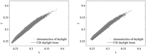
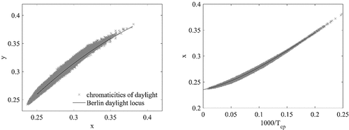
The spectral data were collected in a MySQL-based database and combined with supplemental information, such as solar altitude at the time, luminance and $T_{cp}$ of each of the patches. As in our previous study (Diakite et al. 2018), we compiled two data sets from the database: a 2016 set for modeling, and a 2015 set for validation. The selected data sets were cleaned up using a MATLAB script. Measurements that were faulty by default (e.g. due to maintenance work, repair, and/or device malfunctions) were removed from the data set. Data quality monitoring is ongoing and does not contain uncertainty estimates at this moment. The selected data sets comprised 5348 measurement series with 597,998 daylight spectra for modeling and 4943 measurement series with 538,205 spectra for validation (chromaticities displayed in Fig. 3).

Fig. 3. Chromaticities of daylight in Berlin in the CIE 1931 $x,y$ chromaticity diagram compared to the CIE daylight locus. The diagram on the left shows the modeling data set from the 597,998 SPD measurements gathered in 2016 (left); the one on the right shows the validation data set from the 538,205 SPD measurements gathered in 2015 according to the procedure laid out by the CIE (2018b), limiting the $x_D$ from 0.25 to 0.38 (right).

The following temporal, spatial, and spectral requirements were placed on the compiled data.

3.2.1. Temporal selection

The two full-year data sets were compiled from the database, which allowed an analysis of the spectral sky measurements. The temporal scope for modeling the Berlin daylight locus and determining the corresponding components was limited to the year 2016. This data set covers a wide range of sky conditions, seasons, and times of the day. Due to the homogeneity and the large amount of the data, we expected to be able to accurately determine the daylight locus and the reconstruction procedure. We used the second data set with measurements from 2015 to validate the CIE procedure as well as the locally adjusted procedures. For both modeling and validation, measurements from each day every half hour were selected. To cover a large range of solar altitudes, we considered the hh:15 and hh:45 measurements to create the model, and the hh:00 and hh:30 measurements to validate the model. Only measurements collected after the sun reached a solar altitude greater than 15° (when the appearance of the celestial hemisphere stabilized) were taken into account, to exclude measurement inaccuracies caused by the sun passing through the first degrees of sunrise (Hosek and Wilkie 2012; Knoop et al. 2019b).

3.2.2. Spatial selection

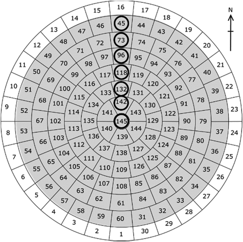
To minimize influences due to haziness and obstructions, we excluded patches with the lowest almucantar (1– 30) from the analysis. This left sky patches 31– 145 (see Tregenza (2004, Fig. 2a, p. 274)) with a minimum almucantar height of 12°. This means that one measuring series for the analysis covered a maximum of 115 sky patches (Fig. 4). The same principles of spatial selection were applied to both the data set for modeling and the data set for validation. Additionally, to examine the impact of atmospheric influences on SPD, we selected seven north-oriented patches on different almucantars, which limited the data set to 33,782 SPD measurements. Figure 4 illustrates the spatial selection.

Fig. 4. Sky patches as defined in Tregenza (1987, 2004) and the CIE (1994). Patches shaded in gray were used for the accuracy analysis and sensitivity study; the patches used to examine atmospheric influences are circled in black.

3.2.3. Spectral selection

We considered wavelengths ranging from 380 nm to 780 nm at 1 nm intervals. We hypothesized that higher resolution compared to the 5 nm intervals used in the CIE reconstruction procedure would result in a more accurate determination of components. We selected measurements with a color temperature between 4000 K and 25,000 K for the spectral, temporal and spatial validation, because these corresponded to the colorimetric ranges of the CIE reconstruction procedure. For the colorimetric and application-related analysis, measurements exceeding 25,000 K were also taken into consideration.

3.3. Data analysis: Modeling

Prior to analyzing locally adapted approaches, the Berlin daylight locus and the components for Berlin were modeled. Both methods use the model data.

3.3.1. Berlin daylight locus

The first set of analyses for the localized approach (Fig. 5) was performed in two stages, and examined the correlation between $x_{D,BLN}$ and $T_{cp}$ on the one hand, and that of the Berlin daylight locus, describing the link between $y_{D,BLN}$ and $x_{D,BLN}$. Altogether, $x$ and $y$ values were calculated for 597,998 SPD measurements collected in 2016. Prior to determining $y_{D,BLN}$, we used a polynomial regression to fit the non-linear relationship between $x_{D,BLN}$ and $T_{cp}$, which resulted in a third-degree polynomial, in line with Judd et al. (1964). Once the regression fit for $x_{D,BLN}$ as a function of $T_{cp}$ was established, it became possible to describe the Berlin daylight locus ($y_{D,BLN}\left(x_{D,BLN}\right)$) using a quadratic polynomial, displayed in Fig. 6. In line with the approach used by Hernández-Andrés et al. (2001a, 2001b), the method of least squares was used to generate both polynomial equations from the data sets. The non-parametric Spearman rank correlation coefficient was used to test the significance of the correlation.

Fig. 5. Diagram of the approach to deriving the Berlin (BLN) daylight chromaticities $x_{D,BLN},y_{D,BLN}.$

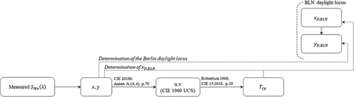
Fig. 6. Non-linear relation between chromaticities of daylight in Berlin (left) and the correlation between the daylight chromaticity coordinate $x_D$ and the inverse correlated color temperature $T_{cp}$ (MK⁻¹) (right).

The third-degree polynomial representing the non-linear relationship between $x_{D,BLN}$ and $T_{cp}$ is illustrated in Fig. 6 and presented in Equation (10)(10) $x_{D,BLN}=\frac{-4.5036\cdot {10}^9}{{T_{cp}}^3}+\frac{2.5225\cdot {10}^6}{{T_{cp}}^2}+\frac{0.22336\cdot {10}^3}{T_{cp}}+0.23535$(10) with a Spearman’s ρ of 1.000.

(10) $x_{D,BLN}=\frac{-4.5036\cdot {10}^9}{{T_{cp}}^3}+\frac{2.5225\cdot {10}^6}{{T_{cp}}^2}+\frac{0.22336\cdot {10}^3}{T_{cp}}+0.23535$(10)

The Berlin daylight locus is expressed by a quadratic polynomial given by Equation (11)(11) ${\mathrm{y}}_{\mathrm{D},\mathrm{B}\mathrm{L}\mathrm{N}}=-2.0795x_{\mathrm{D},\mathrm{B}\mathrm{L}\mathrm{N}}^2+2.2376x_{\mathrm{D},\mathrm{B}\mathrm{L}\mathrm{N}}-0.16974$(11) with a strong correlation reflected in the Spearman’s ρ equal to 0.991.

(11) ${\mathrm{y}}_{\mathrm{D},\mathrm{B}\mathrm{L}\mathrm{N}}=-2.0795x_{\mathrm{D},\mathrm{B}\mathrm{L}\mathrm{N}}^2+2.2376x_{\mathrm{D},\mathrm{B}\mathrm{L}\mathrm{N}}-0.16974$(11)

Figure 7 provides a comparison of whether and to what extent the Berlin daylight locus deviates from the existing CIE daylight locus. Figure 7 also compares our locally adjusted locus with recently determined daylight loci (see Table 1). All loci mainly show different courses at both ends of the $T_{cp}$ range, though not all in the same direction. However, all local loci except the one for Coburg, Australia are above the CIE daylight locus at high $T_{cp}$. The Berlin daylight locus is comparable to the CIE daylight locus between approximately 8000 K and 10,000 K. For $T_{cp}$ higher than 10,000 K, our local locus approaches those of Hernández-Andrés et al. (2001b) (Granada daylight locus based on global spectral irradiance measurements) and Chain (2004) (Vaulx-en-Velin daylight locus based on diffuse spectral irradiance measurements with an aperture angle of 1°); above 15,000 K, the curves are practically identical. Below approximately 8000 K, the Berlin daylight locus deviates from the CIE locus and resembles the Granada daylight locus, which was based on diffuse spectral irradiance measurements with an aperture angle of 1° (Hernández-Andrés et al. 2001a). In the approximate range between 5000 K and up to 25,000 K, the Berlin daylight locus behaves nearly identically to the Nagaoka daylight locus. The course of the Berlin daylight locus, being above the CIE daylight locus at high $T_{cp}$ and below for low $T_{cp}$, most closely resembles those from Bratislava (Rusnák 2014), Vaulx-en-Velin (Chain 2004), and Atsugi (Kobayashi et al. 1996) in its behavior, especially the latter two. The preliminary Berlin daylight locus built on northern sky measurements behaves differently, in particular for low $T_{cp}$.

Fig. 7. Loci of the chromaticities of daylight obtained for different sites along with the CIE daylight locus and the Berlin daylight locus: Granada, Spain (Hernández-Andrés et al. 2001a, 2001b) (upper left); Vaulx-en-Velin, France (Chain 2004) (upper right); Bratislava, Slovakia (Rusnák 2014) (middle left); Berlin, Germany (Diakite et al. 2018) (middle right); Coburg and Bendigo, Australia (Dixon 1978) (lower left); Atsugi and Nagaoka, Japan (Kobayashi et al. 1997, 1996) (lower right).

3.3.2. Berlin components for SPD reconstruction

To address the aforementioned discrepancies between the reconstruction procedure of Judd et al. (1964) and various others (Chain 2004; Diakite et al. 2018; Dixon 1978; Hernández-Andrés et al. 2001a, 2001b; Kobayashi et al. 1997, 1996; Rusnák 2014; Sastri and Das 1968), we calculated Berlin-specific components of the relative SPD of daylight. To do so, we followed various studies (Hernández-Andrés et al. 2001a, 2001b; Judd et al. 1964; Simonds 1963) that used PCA executed in MATLAB to determine the components for Berlin. The components were generated using 597,998 SPDs from the model data set for 2016, under the temporal, spatial, and spectral criteria specified in Section 3.2. The components $S_{0,BLN}\left(\lambda \right)$, $S_{1,BLN}\left(\lambda \right)$, and $S_{2,BLN}\left(\lambda \right)$ are displayed in Fig. 9, and the numerical data can be found in the supplemental material. Figure 8 illustrates the procedure applied.

Fig. 8. Diagram of the procedure of deriving the Berlin components and Berlin weighting factors for SPD reconstruction.

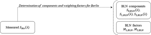
Fig. 9. Components of the daylight distribution S₀(λ), S₁(λ), S₂(λ), CIE (left); Berlin (right).

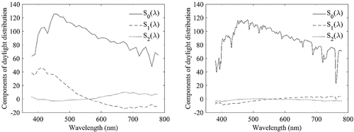
The first three components accounted for 99.91% of all variance in the data set, while six components as suggested by Hernández-Andrés et al. (2001b) for spectrally “almost exact” reconstruction explain 99.99%. Nevertheless, we followed the procedure using three components to correspond to the CIE procedure.

Once the components are derived, any daylight spectrum at any $T_{cp}$ can be represented by a linear combination of these three components: $S_{0,BLN}$, $S_{1,BLN}$ and $S_{2,BLN}$ and their weighting factors $M_{1,BLN}$ and $M_{2,BLN}$, as presented in the following equations:

(12) $S_{BLN}\left(\lambda \right)=S_{0,BLN}\left(\lambda \right)+M_{1,BLN}\cdot S_{1,BLN}\left(\lambda \right)+M_{2,BLN}\cdot S_{2,BLN}\left(\lambda \right)$(12)

where the Berlin weighting factors $M_{1,BLN}$ and $M_{2,BLN}$ resulted in:

$M_{1,BLN}=\frac{5.0767-13.8483\cdot x_D-1.9943\cdot y_D}{0.0157+0.0469\cdot x_D-0.3791\cdot y_D}(13)$

$M_{2,BLN}=\frac{1.3617+61.3011\cdot x_D-62.6447\cdot y_D}{0.0157+0.0469\cdot x_D-0.3791\cdot y_D}(14)$

In line with the CIE (2018b) procedure, the first component $S_{0,BLN}\left(\lambda \right)$ was set to 100 and the values of the second and third components $S_{1,BLN}\left(\lambda \right)$ and $S_{2,BLN}\left(\lambda \right)$ equaled 0 at the normalizing wavelength of 560 nm. Within the wavelength range under study, the slope of the curves of the components $S_{1,BLN}\left(\lambda \right)$ and $S_{2,BLN}\left(\lambda \right)$ significantly diverge in direction from those of most previous studies (Dixon 1978; Kobayashi et al. 1997, 1996; Rusnák 2014; Sastri and Das 1968), yet are consistent with those of Hernández-Andrés et al. (2001b). Due to the higher resolution of the measurement data, the components for Berlin exhibit more variation (best recognizable in the first component $S_{0,BLN}$), which supports a more accurate reconstruction.

3.4. Data analysis: Validation

In the validation process, we examined whether and with what goodness-of-fit the CIE (2018b) method could be used to reconstruct the SPD of daylight for Berlin. Subsequently, two locally adapted approaches were developed and compared with the CIE method in order to examine if the adjusted reconstructions performed more accurately. The first reconstruction approach, hereafter referred to as BLN₁, used daylight chromaticities adapted to Berlin: the Berlin daylight locus $y_{D,BLN}\left(x_{D,BLN}\right)$ with an adjusted $x_{D,BLN}\left(T_{cp}\right)$. The second approach, hereafter called BLN₂, included, in addition to the Berlin-adapted daylight chromaticities, locally adjusted components ($S_{0,BLN}$, $S_{1,BLN}$, and $S_{2,BLN}$) and their corresponding factors ($M_{1,BLN}$ and $M_{2,BLN}$) calculated for Berlin. We used the $\mathrm{G}\mathrm{F}\mathrm{C}$ to test the accuracy of the reconstructions in all cases. All statistical analyses were performed in MATLAB, with the methods validated using the measurement series from 2015. The reconstruction procedure is diagrammed in Fig. 10; the adjustments incorporated into each approach in Table 2.

Fig. 10. Diagram of the reconstruction procedure.

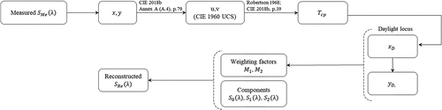
3.4.1. Reconstruction based on the CIE method

To use the CIE method for reconstruction of daylight spectra (see Fig. 1 and Table 2), it was first necessary, to determine the $T_{cp}$. The $T_{cp}$ values were determined according to Robertson (1968) using the spectral distributions collected in 2015. Subsequently, the $x_{D,CIE}$ chromaticity coordinates on the CIE daylight locus were calculated from the $T_{cp}$, defining the $y_{D,CIE}$ chromaticity coordinates by means of the CIE daylight locus. We then used the $x_{D,CIE},y_{D,CIE}$ coordinates together to calculate the factors $M_{1,CIE}$ and $M_{2,CIE}$, to eventually reconstruct the daylight spectrum using the components $S_{0,CIE}$, $S_{1,CIE}$, and $S_{2,CIE}$ as tabulated in CIE (2018b). The accuracy of the reconstruction using the CIE procedure was tested using the $\mathrm{G}\mathrm{F}\mathrm{C}$, in line with Hernández-Andrés et al. (2001b).

3.4.2. Reconstruction based on the locally adjusted methods

As shown in Table 2, there were two different adjustment levels for the local procedure: BLN₁ and BLN₂.

3.4.2.1. Modified reconstruction by means of the Berlin daylight locus (BLN₁)

Since the daylight locus is based on chromaticities, in contrast to the daylight components that use spectral information, it is relatively easy and cost-effective to determine local loci for different locations. Therefore, we first verified whether reconstruction was significantly improved by “only” replacing the CIE daylight locus with a local daylight locus. Once the polynomial equations for the Berlin daylight locus $y_{D,BLN}$ and $x_{D,BLN}$ were established, it was possible to calculate $x_{D,BLN}$ values on the Berlin daylight locus from the $T_{cp}$, which had been defined for the 2015 spectral measurements. To correspond with the CIE method, the next step in reconstructing the daylight spectra was to incorporate the CIE factors $M_{1,CIE}$ and $M_{2,CIE}$ and the CIE components $S_{0,CIE}$, $S_{1,CIE}$, and $S_{2,CIE}$. This localized method, where the only modification was to incorporate the Berlin daylight locus, is hereafter referred to as BLN₁.

3.4.2.2. Modified reconstruction by means of the Berlin daylight locus as well as Berlin-specific components (BLN₂)

The next step was to examine to what extent locally adapted components could improve the accuracy of the reconstruction. Therefore, the BLN₂ reconstruction method extends BLN₁ by additionally adjusting the CIE components with local components – $S_{0,BLN}$, $S_{1,BLN}$, and $S_{2,BLN}$ and their weighting factors $M_{1,BLN}$ and $M_{2,BLN}$. This localized method, incorporating the Berlin daylight locus as well as Berlin-specific components, is hereafter referred to as BLN₂.

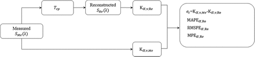
3.4.3. Accuracy assessment of the reconstruction methods

We quantitatively assessed the accuracy of the reconstruction for the three reconstruction methods applied by using the Goodness-of-Fit Coefficient ($\mathrm{G}\mathrm{F}\mathrm{C}$) as described in Hernández-Andrés et al. (2001b) This was calculated as follows:

$\mathrm{G}\mathrm{F}\mathrm{C}=\frac{{\sum }_{i=380}^{780}{S}_{Me}\left({\lambda }_i\right)\cdot S_{Re}\left({\lambda }_i\right)}{\sqrt{{\sum }_{i=380}^{780}{[S_{Me}\left({\lambda }_i\right)]}^2}\cdot \sqrt{{\sum }_{i=380}^{780}{[S_{Re}\left({\lambda }_i\right)]}^2}}(15)$

where $S_{Me}\left(\lambda \right)$corresponds to the measured SPD and $S_{Re}\left(\lambda \right)$to the reconstructed SPD at a particular $T_{cp}$. $\mathrm{G}\mathrm{F}\mathrm{C}$ varies between 0 and 1, where $\mathrm{G}\mathrm{F}\mathrm{C}=1$ represents an exact reconstruction. According to Hernández-Andrés et al. (2001b), reconstructions can be classified into the following categories:

$\mathrm{G}\mathrm{F}\mathrm{C}\ge 0.9950\stackrel{\wedge }{=}\mathrm{c}\mathrm{o}\mathrm{l}\mathrm{o}\mathrm{r}\mathrm{i}\mathrm{m}\mathrm{e}\mathrm{t}\mathrm{r}\mathrm{i}\mathrm{c}\mathrm{a}\mathrm{l}\mathrm{l}\mathrm{y}\mathrm{a}\mathrm{c}\mathrm{c}\mathrm{u}\mathrm{r}\mathrm{a}\mathrm{t}\mathrm{e}\mathrm{r}\mathrm{e}\mathrm{c}\mathrm{o}\mathrm{n}\mathrm{s}\mathrm{t}\mathrm{r}\mathrm{u}\mathrm{c}\mathrm{t}\mathrm{i}\mathrm{o}\mathrm{n}$

$\mathrm{G}\mathrm{F}\mathrm{C}\ge 0.9990\stackrel{\wedge }{=}\mathrm{g}\mathrm{o}\mathrm{o}\mathrm{d}\mathrm{r}\mathrm{e}\mathrm{c}\mathrm{o}\mathrm{n}\mathrm{s}\mathrm{t}\mathrm{r}\mathrm{u}\mathrm{c}\mathrm{t}\mathrm{i}\mathrm{o}\mathrm{n}$

$\mathrm{G}\mathrm{F}\mathrm{C}\ge 0.9999\stackrel{\wedge }{=}\mathrm{e}\mathrm{x}\mathrm{a}\mathrm{c}\mathrm{t}\mathrm{r}\mathrm{e}\mathrm{c}\mathrm{o}\mathrm{n}\mathrm{s}\mathrm{t}\mathrm{r}\mathrm{u}\mathrm{c}\mathrm{t}\mathrm{i}\mathrm{o}\mathrm{n}$

Next, we used the $\mathrm{G}\mathrm{F}\mathrm{C}$ to determine the accuracy of the reconstructions for all three methods. The approach is shown in Fig. 11. $\mathrm{G}\mathrm{F}\mathrm{C}$ were also calculated as a function of wavelength range, season, $T_{cp}$, sky conditions (represented by 15 CIE Standard General Sky Types categorized into three sky conditions: overcast (CIE Sky Type 1–5), intermediate (CIE Sky Type 6–10), and clear (CIE Sky Type 11–15)), and atmospheric influences.

Fig. 11. Diagram of the approach to determine the Goodness-of-Fit Coefficient ($GFC$) of the CIE reconstruction procedure and locally adjusted procedures (BLN₁ and BLN₂).

3.5. Data analysis: Application

The final step was to examine the extent to which the anticipated increase in accuracy due to local adjustments of the reconstruction procedure affected the accuracy of NIF assessments. Although NIF responses caused by ocular exposure to daylight during the daytime are not well understood yet, it is almost certain that NIF effects are a result of the combined responses of all retinal photoreceptors (Lucas et al. 2014; Schlangen and Price 2021; Souman et al. 2018; Wirz-Justice et al. 2020; Zeitzer 2018). In other words, intrinsically-photosensitive retinal ganglion cells (ipRGCs), rods, and cones all contribute to NIF effects. To account for this, we used α-opic weighted irradiances according to CIE (2018a) to quantify light for NIF responses. For the reconstruction procedures, the $T_{cp}$ corresponding to the measured spectrum $S_{Me}\left(\lambda \right)$ was calculated for each measurement of the 2015 data set. This was followed by reconstructing the spectrum $S_{Re}\left(\lambda \right)$ and determining the corresponding α-opic efficacy of luminous radiation (α-opic ELR) $K_{\alpha ,v,Re}$ for each referred reconstruction. The α-opic efficacy of luminous radiation $K_{\alpha ,v,Me}$ matching the measurement was calculated concurrently. The $K_{\alpha ,v}$ corresponding to the measured and reconstructed spectra were compared using $\mathrm{M}\mathrm{A}\mathrm{P}{\mathrm{E}}_{\alpha }$, $\mathrm{R}\mathrm{M}\mathrm{S}\mathrm{P}{\mathrm{E}}_{\alpha }$, and $\mathrm{M}\mathrm{P}{\mathrm{E}}_{\alpha }$ as follows:

(16) $\mathrm{M}\mathrm{A}\mathrm{P}{\mathrm{E}}_{\alpha }=100\cdot \frac{1}{\mathrm{n}}\sum \left|\frac{{\mathrm{e}}_{\mathrm{t}}}{{\mathrm{d}}_{\mathrm{t}}}\right|$(16)

(17) $\mathrm{R}\mathrm{M}\mathrm{S}\mathrm{P}{\mathrm{E}}_{\alpha }=100\cdot \sqrt{\frac{1}{\mathrm{n}}\sum {\left(\frac{{\mathrm{e}}_{\mathrm{t}}}{{\mathrm{d}}_{\mathrm{t}}}\right)}^2}$(17)

(18) $\mathrm{M}\mathrm{P}{\mathrm{E}}_{\alpha }=100\cdot \frac{1}{\mathrm{n}}\sum \frac{{\mathrm{e}}_{\mathrm{t}}}{{\mathrm{d}}_{\mathrm{t}}}$(18)

$e_t$= $K_{\alpha ,v,Me}$- $K_{\alpha ,v,Re}$, where $K_{\alpha ,v,Re}$ stands for ${\mathrm{K}}_{\alpha ,\mathrm{v},\mathrm{C}\mathrm{I}\mathrm{E}}$ or ${\mathrm{K}}_{\alpha ,\mathrm{v},\mathrm{B}\mathrm{L}\mathrm{N}}$ and $d_t$= $K_{\alpha ,v,Me}$

For this part of the study, it was necessary to categorize the measurements into $T_{cp}$ ranges in accordance with Robertson (1968) and transform them according to Diakite-Kortlever and Knoop (2021). This resulted in eight intervals, ranging at $T_{cp}$ values from 4000 K to 1,000,000 K. Tables 7–9 below list the categories and their corresponding $T_{cp}$ intervals. The categories are built on inverse $T_{cp}$, described by micro-reciprocal-degree MIRED (MK⁻¹), since the Kelvin scale does not account for the non-linear color perceptibility of the human eye. However, the intervals are labeled in the Kelvin scale for ease of reading.

Table 7. Mean absolute percentage error $\mathrm{M}\mathrm{A}\mathrm{P}{\mathrm{E}}_{\alpha }$ [%] for α-opic quantities

$\mathrm{M}\mathrm{A}\mathrm{P}{\mathrm{E}}_{\alpha }$	Melanopic			S-cone-opic			M-cone-opic			L-cone-opic			Rhodopic
$T_{cp}$ range	CIE	BLN1	BLN2	CIE	BLN1	BLN2	CIE	BLN1	BLN2	CIE	BLN1	BLN2	CIE	BLN1	BLN2
4000 $<T_{cp}\le$ 5000	0.7	0.5	0.3	1.6	2.8	2.9	0.1	0.1	0.1	0.1	0.1	0.1	0.4	0.3	0.2
5000 $<T_{cp}\le$ 6667	0.5	0.4	0.4	1.2	0.6	0.7	0.1	0.1	0.1	0.1	0.1	0.1	0.3	0.3	0.3
6667 $<T_{cp}\le$ 10,000	0.4	0.3	0.3	1.1	0.8	0.9	0.2	0.2	0.2	0.1	0.1	0.1	0.3	0.3	0.3
10,000$<T_{cp}\le$ 12,500	0.3	0.3	0.3	0.7	0.7	0.7	0.2	0.2	0.2	0.1	0.1	0.1	0.3	0.3	0.3
12,500 $<T_{cp}\le$ 16,667	0.4	0.4	0.4	0.6	0.5	0.5	0.3	0.2	0.2	0.2	0.1	0.1	0.4	0.4	0.4
16,667 $<T_{cp}\le$ 25,000	0.5	0.5	0.4	0.6	0.6	0.5	0.3	0.3	0.2	0.3	0.1	0.1	0.4	0.5	0.4
25,000 $<T_{cp}\le$ 50,000	0.6	0.4	0.6	0.5	1.0	0.7	0.3	0.2	0.2	0.3	0.1	0.1	0.4	0.4	0.5
50,000 $<T_{cp}\le$ 1,000,000	0.5	0.3	1.1	0.4	1.7	1.4	0.3	0.2	0.2	0.4	0.1	0.1	0.3	0.3	1.0

Table 8. Root mean square percentage error $\mathrm{R}\mathrm{M}\mathrm{S}\mathrm{P}{\mathrm{E}}_{\alpha }$ [%] for α-opic quantities

$\mathrm{R}\mathrm{M}\mathrm{S}\mathrm{P}{\mathrm{E}}_{\alpha }$	Melanopic			S-cone-opic			M-cone-opic			L-cone-opic			Rhodopic
$T_{cp}$ range	CIE	BLN1	BLN2	CIE	BLN1	BLN2	CIE	BLN1	BLN2	CIE	BLN1	BLN2	CIE	BLN1	BLN2
4000 $<T_{cp}\le$ 5000	0.8	0.7	0.4	2.3	3.2	3.2	0.1	0.1	0.1	0.1	0.1	0.1	0.5	0.4	0.3
5000 $<T_{cp}\le$ 6667	0.6	0.5	0.5	1.3	0.9	0.9	0.1	0.1	0.1	0.1	0.1	0.1	0.4	0.3	0.3
6667 $<T_{cp}\le$ 10,000	0.5	0.4	0.4	1.3	1.1	1.2	0.2	0.2	0.2	0.1	0.1	0.1	0.4	0.4	0.4
10,000 $<T_{cp}\le$ 12,500	0.4	0.4	0.4	0.9	0.9	0.9	0.3	0.3	0.3	0.2	0.1	0.1	0.4	0.4	0.4
12,500 $<T_{cp}\le$ 16,667	0.5	0.5	0.5	0.8	0.7	0.7	0.3	0.3	0.3	0.2	0.1	0.1	0.4	0.5	0.5
16,667 $<T_{cp}\le$ 25,000	0.6	0.6	0.6	0.8	0.7	0.6	0.4	0.3	0.3	0.3	0.1	0.1	0.5	0.5	0.5
25,000 $<T_{cp}\le$ 50,000	0.7	0.5	0.7	0.6	1.0	0.8	0.3	0.3	0.2	0.4	0.1	0.1	0.5	0.5	0.7
50,000 $<T_{cp}\le$ 1,000,000	0.6	0.4	1.2	0.5	1.7	1.4	0.4	0.2	0.3	0.4	0.1	0.1	0.4	0.4	1.0

Table 9. Mean percentage error $\mathrm{M}\mathrm{P}{\mathrm{E}}_{\alpha }$ [%] for the α-opic quantities

$\mathrm{M}\mathrm{P}{\mathrm{E}}_{\alpha }$	Melanopic			S-cone-opic			M-cone-opic			L-cone-opic			Rhodopic
$T_{cp}$ range	CIE	BLN1	BLN2	CIE	BLN1	BLN2	CIE	BLN1	BLN2	CIE	BLN1	BLN2	CIE	BLN1	BLN2
4000 $<T_{cp}\le$ 5000	0.7	−0.5	−0.1	1.0	−2,4	−2,5	0.1	0.0	0.1	0.1	−0.1	−0.1	0.4	−0.3	0.1
5000$<T_{cp}\le$ 6667	0.4	−0.1	−0.2	1.1	−0.5	−0.5	0.0	0.1	0.0	0.1	0.0	−0.1	0.2	0.0	0.0
6667 $<T_{cp}\le$ 10,000	0.3	0.1	0.0	0.5	−0.3	−0.4	0.0	0.0	0.0	0.0	0.0	0.0	0.2	0.1	0.1
10,000 $<T_{cp}\le$ 12,500	−0.1	−0.1	0.1	−0.4	−0.3	−0.4	0.1	0.0	0.0	−0.1	−0.1	0.0	0.0	−0.1	0.1
12,500 $<T_{cp}\le$ 16,667	−0.2	−0.2	0.2	−0.5	0.0	−0.1	0.2	−0.1	0.0	−0.2	0.0	0.0	−0.1	−0.2	0.2
16,667 $<T_{cp}\le$ 25,000	−0.4	−0.3	0.3	−0.5	0.4	0.2	0.2	−0.1	0.0	−0.3	0.0	0.0	−0.2	−0.3	0.3
25,000 $<T_{cp}\le$ 50,000	−0.5	−0.2	0.6	−0.5	0.9	0.7	0.3	−0.1	0.1	−0.3	0.0	0.0	−0.3	−0.2	0.5
50,000 $<T_{cp}\le$ 1,000,000	−0.5	0.2	1.1	−0.4	1.7	1.4	0.3	0.0	0.2	−0.4	0.0	0.1	−0.2	0.1	1.0

A diagram of the analysis process is illustrated in Fig. 12. The total number of spectra subject to this analysis were 547,772 from 4943 measurement series.

Fig. 12. Diagram of the approaches for the sensitivity study.

4. Results

The results section is twofold: the first consists of a comparative analysis to study the accuracy of the three reconstruction procedures (validation), and the second a sensitivity study to identify the impact of the accuracy of the reconstructions on actual application (NIF assessment).

4.1. Comparison of the accuracy of the reconstruction procedures

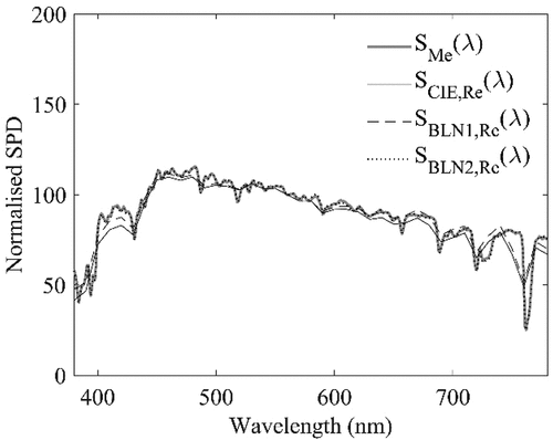
4.1.1. Spectral analysis: best reconstruction, mean(GFC), and GFC as a function of wavelength

Figure 13 depicts the measurement with the highest achieved $max\left(\mathrm{G}\mathrm{F}{\mathrm{C}}_{\mathrm{B}\mathrm{L}\mathrm{N}2}\right)=0.99998$, and the reconstructions of the SPD for all three methods as a sample case. It is apparent from the graph that the method optimized for Berlin with locally adjusted components (BLN₂) reconstructs the daylight spectrum with the finest resolution. The deviations are minimal and the wavelength-dependent variations in SPD (peaks) are well reproduced due to the higher resolution ($\mathrm{\Delta }\lambda =1nm$). An exact reconstruction ($GFC\ge 0.9999$) is achieved with neither the CIE nor the BLN₁ method for this data set.

Fig. 13. Normalized measured spectral irradiance (-, gray, $S_{Me}\left(\lambda \right)$) with the best achieved $max\left(\mathrm{G}\mathrm{F}{\mathrm{C}}_{\mathrm{B}\mathrm{L}\mathrm{N}2}\right)=0.99998$ conducted on 10 September 2015, at 14:58:13 CEST, with a solar altitude of 37.17°, for sky patch 114, with a $T_{cp}$ equal to 6016 K (overcast sky) compared to the corresponding reconstructions performed using: the CIE method (-, $S_{CIE,Re}\left(\lambda \right)$); the BLN₁ method, using $x_{D,BLN},y_{D,BLN}$(--,$S_{BLN1,Re}\left(\lambda \right)$); and the BLN₂ method, using $x_{D,BLN},y_{D,BLN}$ and components of the daylight distribution $S_{0,BLN}$, $S_{1,BLN}$, and $S_{2,BLN}$ (:, $S_{BLN2,Re}\left(\lambda \right)$).

This was followed by determining the percentage of colorimetrically “accurate” ($GFC\ge 0.9950$), “good” ($GFC\ge 0.9990$), and “exact” ($GFC\ge 0.9999$) reconstructions (Table 3). From the 538,205 SPDs on which the validation was based, 99.72% of the reconstructions using the BLN₂ method, 96.44% using the BLN₁ method and 95.97% using the CIE method could be classified as colorimetrically “accurate.” However, only the Berlin method BLN₂ achieved “exact” reconstructions (2.58%). Moreover, more than half (67.74%) of the reconstitutions qualified as “good” using the BLN₂ method, whereas for both the CIE and the BLN₁ procedure, “good” reconstructions only amounted to 0.004% and 0.01%, respectively.

To assess the accuracy of the reconstruction, the arithmetic mean of the $\mathrm{G}\mathrm{F}\mathrm{C}$ was calculated for all methods (Table 4). For the optimized method BLN₂, the $\mathrm{m}\mathrm{e}\mathrm{a}\mathrm{n}\left(\mathrm{G}\mathrm{F}{\mathrm{C}}_{\mathrm{B}\mathrm{L}\mathrm{N}2}\right)=0.9991$ can be therefore classified as colorimetrically “good,” whereas the $\mathrm{m}\mathrm{e}\mathrm{a}\mathrm{n}\left(\mathrm{G}\mathrm{F}\mathrm{C}\right)$ values for the CIE and the BLN₁ method of 0.9969 and 0.9971, respectively, could only be classified as colorimetrically “accurate.” The next step was to determine $\mathrm{m}\mathrm{e}\mathrm{a}\mathrm{n}\left(\mathrm{G}\mathrm{F}\mathrm{C}\right)$ values for different wavelength ranges (Table 4), using the wavelength classification ranges found in Rossotti (1983). The evaluation showed that, for all methods, reconstructions increasingly deviated as wavelengths increased (greater than 585 nm), and only the BLN₂ method fulfilled the requirements for an accurate reconstruction. In contrast, the wavelength range between 490 nm and 585 nm showed the highest $\mathrm{m}\mathrm{e}\mathrm{a}\mathrm{n}\left(\mathrm{G}\mathrm{F}\mathrm{C}\right)$ values, resulting in “good” reconstructions for all three methods. Still, the BLN₂ method yielded the best results. Similarly, in the lower wavelengths ($380\mathrm{n}\mathrm{m}\le \lambda \le 490\mathrm{n}\mathrm{m}$), the BLN₁ and CIE methods reproduced daylight SPDs that were on average colorimetrically “accurate,” yet the BLN₂ method delivered better results, with a mean classification as colorimetrically “good.”

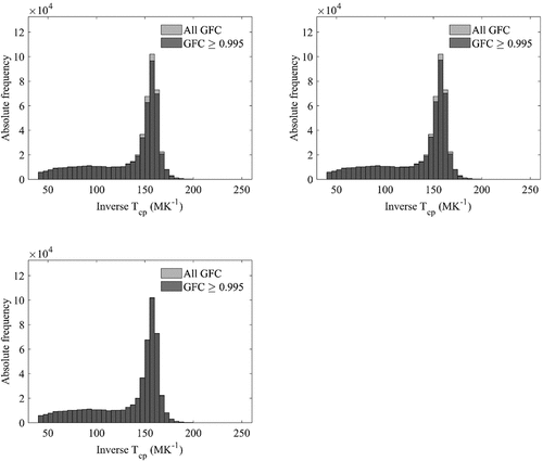
4.1.2. Colorimetric analysis: Accuracy as a function of ${\mathit{T}}_{\mathbf{c}\mathbf{p}}$

As part of the colorimetric analysis, we evaluated the $\mathrm{G}\mathrm{F}\mathrm{C}$ as a function of the $T_{cp}$. To do so, the validation data set was expanded to include measurements with $T_{cp}>25,000\mathrm{K}$, which increased the total number of analyzed spectra to 547,772. The histograms in Fig. 14 represent the frequency distributions of inverse $T_{cp}$, presented in MIRED (MK⁻¹) for an interval of 5 MK⁻¹ and the percentage of reconstructions with a $\mathrm{G}\mathrm{F}\mathrm{C}$ greater than or equal to 0.9950. Due to the predominantly overcast sky conditions in Berlin, the dominant $T_{cp}$ is 155 MK⁻¹ to 160 MK⁻¹ (approximately 6250 K to 6450 K). At that range, the CIE method indeed provided a colorimetrically “accurate” reconstruction for over 94% of the results. The worst reconstruction accuracy occurred for low $T_{cp}$ values. The BLN₁ procedure resembled the CIE procedure in its behavior, providing marginally better results for higher $T_{cp}$ and insignificantly worse ones for lower $T_{cp}$. The Berlin-adapted BLN₂ method not only reconstructed the spectrum in the dominant range better (99.69%), but also provided comparably good results (> 99%) throughout the whole $T_{cp}$ range.

Fig. 14. Goodness-of-fit of the reconstructions as expressed by $GFC\ge 0.9950$, as a function of the inverse correlated color temperature $T_{cp}$. Upper left, calculated using the CIE method; upper right, the BLN₁ method, using $x_{D,BLN},y_{D,BLN}$; and lower left, the BLN₂ method, using $x_{D,BLN},y_{D,BLN}$ and the components $S_{0,BLN}$, $S_{1,BLN}$, and $S_{2,BLN}$. The numerical data of the percentages of colorimetrically accurate reconstructions can be found in the supplemental material.

4.1.3. Temporal analysis: Accuracy as a function of sky conditions and seasons

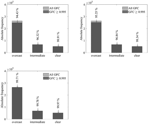
Other factors that might hypothetically influence the quality of the reconstruction are sky conditions, and therefore the corresponding sky type and seasonal variations. Based on the 15 luminance sky types defined by the CIE (2003), we analyzed the relationship between the reconstructions and the measured sky types. For this purpose, we limited our measurements to those that corresponded to a CIE General Standard Sky Type in line with Kobav et al. (2013), which reduced the data set for this assessment to 384,893 SPDs. Next, the CIE Sky Types were classified into three categories of sky conditions: overcast (CIE Sky Types 1–5, with 264,233 SPDs), intermediate (CIE Sky Types 6–10, with 68,743 SPDs), and clear (CIE Sky Types 11–15, with 51,917 SPDs). The histograms in Fig. 15 show the quality of the reconstructions as a function of sky conditions when using the CIE and the Berlin-adapted procedures. The CIE reconstruction method gives slightly better results for clear skies (over 98% reconstructions with $\mathrm{G}\mathrm{F}\mathrm{C}\ge 0.9950$) than for partly cloudy (approximately 96%) and overcast skies (approximately 94%). Since the $T_{cp}$ of an overcast sky in Berlin for this data set is 6614 K ± 481 K (calculated for CIE Sky Types 1–5), this result correlates well with the observations from Section 4.1.2, where the worst reconstruction accuracies were found for lower $T_{cp}$ values. The proportions of colorimetrically “accurate” reconstructions for different sky types using the Berlin BLN₂ method are almost identical for all $T_{cp}$ ranges (> 99%). The results of the BLN₁ method were similar to those using the CIE procedure (overcast skies 95%, intermediate skies 96%, and clear skies 98%). Table 5 lists the $\mathrm{m}\mathrm{e}\mathrm{a}\mathrm{n}\left(\mathrm{G}\mathrm{F}\mathrm{C}\right)$ values, highlighting the better reconstruction of the BLN₂ procedure for overcast and intermediate skies as well as a slightly higher $\mathrm{m}\mathrm{e}\mathrm{a}\mathrm{n}\left(\mathrm{G}\mathrm{F}\mathrm{C}\right)$ for clear skies, though the average reconstruction continued to be classified as “accurate.”

Fig. 15. Percentage of colorimetrically “accurate” ($GFC\ge 0.9950$) reconstructions according to sky conditions for each of the three methods. Upper left, the CIE method; upper right, the BLN₁ method ($x_{D,BLN},y_{D,BLN}$); and lower left, the BLN₂ method ($x_{D,BLN},y_{D,BLN}$ and components $S_{0,BLN}$, $S_{1,BLN}$, and $S_{2,BLN}$). The values above the bars indicate the percentage of colorimetrically “accurate” ($GFC\ge 0.9950$) reconstructions.

We used two periods to study the impact of seasonal variations on spectral reconstruction: summer (comprising 144,517 measurements of the validation set taken in June, July, and August) and winter (comprising 46,356 measurements taken in December, January, and February). As indicated in Table 6, no significant changes in $\mathrm{m}\mathrm{e}\mathrm{a}\mathrm{n}\left(\mathrm{G}\mathrm{F}\mathrm{C}\right)$ or any clear trends can be observed. Here too, the BLN₂ method returns the best results.

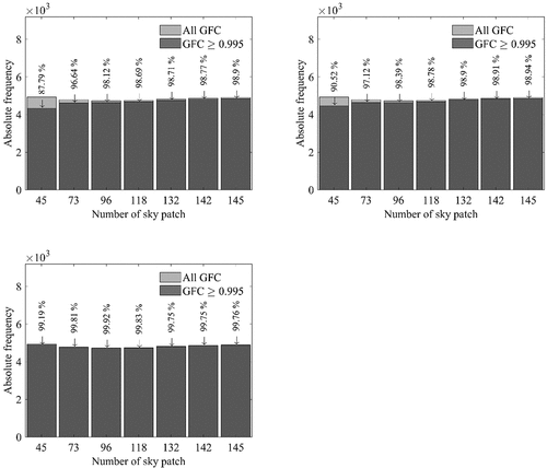
4.1.4. Spatial analysis: Accuracy as a function of atmospheric conditions

The analysis of lower almucantars investigating atmospheric conditions focused on six patches due north and the zenith with a total of 33,782 spectra (see Fig. 4). As Fig. 16 suggests, having a position close to the horizon, represented here by Patch no. 45 (2^nd almucantar), indeed has an effect on the accuracy of the CIE procedure and therefore of the BLN₁ procedure as well, where approximately 10% of the reconstructions in this patch were inaccurate. However, sky position shows no significant effect on the accuracy of the BLN₂ procedure, where inaccurate reconstructions were lower than 1% for all patch heights. We obtained similar results from observations to the south. An additional analysis with a validation data set limited to the patches above Tregenza’s second almucantar (Patches 61–145, see Fig. 4) resulting in 397,582 SPDs revealed no significant improvement in $\mathrm{m}\mathrm{e}\mathrm{a}\mathrm{n}\left(\mathrm{G}\mathrm{F}\mathrm{C}\right)$ for any of the three methods, with $\mathrm{m}\mathrm{e}\mathrm{a}\mathrm{n}\left(\mathrm{G}\mathrm{F}{\mathrm{C}}_{\mathrm{C}\mathrm{I}\mathrm{E}}\right)=0.99718$, $\mathrm{m}\mathrm{e}\mathrm{a}\mathrm{n}\left(\mathrm{G}\mathrm{F}{\mathrm{C}}_{\mathrm{B}\mathrm{L}\mathrm{N}1}\right)=0.99733$, and $\mathrm{m}\mathrm{e}\mathrm{a}\mathrm{n}\left(\mathrm{G}\mathrm{F}{\mathrm{C}}_{\mathrm{B}\mathrm{L}\mathrm{N}2}\right)=0.99921$.

Fig. 16. Percentage of colorimetrically “accurate” ($GFC\ge 0.9950$) reconstructions according to seven sky patches (north and zenith direction, nos. 45, 73, 96, 118, 132, 142, 145). Upper left, the CIE method; upper right, the BLN₁ method (using $x_{D,BLN},y_{D,BLN}$); and lower left, the BLN₂ method (using $x_{D,BLN},y_{D,BLN}$ and components $S_{0,BLN}$, $S_{1,BLN}$, and $S_{2,BLN}$). The values above the bars indicate the percentage of colorimetrically “accurate” ($GFC\ge 0.9950$) reconstructions.

4.2. Sensitivity study: NIF assessment

In this section, we measured the performance of the three reconstruction procedures in the context of NIF responses. Within the $T_{cp}$ range between 4000 K and 25,000 K, which corresponds to the boundaries outlined in the CIE reconstruction procedure, the BLN₂ procedure performs best for almost all receptors. However, all three procedures performed well, with $\mathrm{M}\mathrm{A}\mathrm{P}{\mathrm{E}}_{\alpha }$ and $\mathrm{R}\mathrm{M}\mathrm{S}\mathrm{P}{\mathrm{E}}_{\alpha }$ values lower than 1% for all receptors except S-cones. Moreover, $max\left(\mathrm{M}\mathrm{A}\mathrm{P}{\mathrm{E}}_{\alpha }\right)$ and $max\left(\mathrm{R}\mathrm{M}\mathrm{S}\mathrm{P}{\mathrm{E}}_{\alpha }\right)$ never exceeded 3% and 4%, respectively, for any receptors. For $T_{cp}$ greater than 25,000 K, the BLN₂ procedure yielded the highest melanopic $\mathrm{M}\mathrm{A}\mathrm{P}{\mathrm{E}}_{\alpha }$ and $\mathrm{R}\mathrm{M}\mathrm{S}\mathrm{P}{\mathrm{E}}_{\alpha }$ of all three procedures. Yet even in this range, the $\mathrm{M}\mathrm{A}\mathrm{P}{\mathrm{E}}_{\alpha }$ and $\mathrm{R}\mathrm{M}\mathrm{S}\mathrm{P}{\mathrm{E}}_{\alpha }$ did not exceed 2%. Differences between the CIE and the optimized procedures are therefore negligible. Thus, all three procedures are “accurate” in prediction for all five receptors. The results are presented in Tables 7–9.

5. Discussion

One initial objective of this study was to determine whether localized procedures could reconstruct daylight SPD patterns more accurately than the prevailing CIE procedure. The first part of this study was therefore to determine what effect local adjustments of the daylight chromaticity coordinates $x_D,y_D$ (daylight locus) as well as of localized PCA components and their weighing factors had on the accuracy of the reconstruction procedures. We also hypothesized that other factors, such as wavelength and $T_{cp}$ range, sky and atmospheric conditions, as well as seasonal changes might affect the accuracy of the reconstruction. The second part of the study was designed to determine what implications reconstruction accuracy has for practical application – in this case, for NIF assessment. To do so, we examined how significantly various spectral profiles of daylight stimulate the five retinal photoreceptors that contribute to NIF responses.

5.1. The accuracy of the reconstruction procedures and its implications for NIF assessment

Our current results corroborate the hypothesis that a localized procedure can improve the accuracy of the SPD reconstruction in terms of yielding a higher number of “accurate,” “good,” and “exact” reconstructions, confirming earlier findings by Hernández-Andrés et al. (2001a, 2001b). Moreover, as Tourasse and Dumortier (2015) have noted, the improvement of accuracy seems to depend to a larger extent on the components and their weighting factors than on the daylight locus. Adjusting the daylight locus alone (BLN₁) is not sufficient to achieve significant differences in reconstruction accuracy. Although the amount of accurate and good reconstructions is slightly higher, the difference is negligible; the procedure still yields the same $\mathrm{m}\mathrm{e}\mathrm{a}\mathrm{n}\left(\mathrm{G}\mathrm{F}\mathrm{C}\right)$ as that of the CIE procedure. This result is in line with the study by Chain (2004). This could be a result of the relative similarity between the Berlin daylight locus and the CIE daylight locus, and might not be the case for locations with deviating daylight loci. Nonetheless, this is partially in agreement with the previous literature, where the results have been ambiguous. These incongruities in daylight loci might be attributed to inconsistency in measurement approaches. The extensive variations in equipment and methods to measure daylight were discussed by Knoop et al. (2019b); this ultimately resulted in a measurement and documentation template – a roadmap for reporting spectral measurements. A coherent measurement campaign as Knoop et al. (2019b) proposed would be beneficial in broadening current understanding of site-dependent differences in daylight profiles, if any, and in creating a uniform basis for spectral daylight data.

Several studies (Hernández-Andrés et al. 2001a, 2001b; Rusnák 2014) have criticized the performance of the CIE reconstruction method at high $T_{cp}$. Our analysis of the accuracy as a function of wavelength also indicated that shorter and longer wavelengths of light are not represented as accurately as the intermediate wavelength range. This might affect reconstructions for SPDs with higher $T_{cp}$ values, because these are characterized by more prominent short-wavelength components and smaller long-wavelength components. However, a complementary analysis of the $\mathrm{G}\mathrm{F}\mathrm{C}$ as a function of the $T_{cp}$ challenged prior results, revealing that none of the procedures outlined here had a significant effect on the reconstruction accuracy at higher $T_{cp}$ (> 25,000 K). It is therefore noteworthy and somewhat counterintuitive that the CIE and BLN₁ procedures generated higher $\mathrm{m}\mathrm{e}\mathrm{a}\mathrm{n}\left(\mathrm{G}\mathrm{F}\mathrm{C}\right)$ values for clear skies than for overcast skies. In contrast, the BLN₂ procedure, which employed spatially resolved measurements and therefore contained $T_{cp}$ values greater than 25,000 K, not only performed generally better under both sky conditions, but excelled for overcast skies. One possible explanation for this might be that the BLN₂ procedure is derived from a data set dominated by data on overcast skies. The overrepresentation is caused by the natural frequency of occurrence of overcast skies at this location, as shown in Fig. 15. An identical number of randomized correlated color temperatures and therefore SPDs would be advantageous to achieve equal weighting.

As detailed in the literature review, Chain (2004) suggested that atmospheric conditions may also influence the accuracy of SPD reconstruction. Similarly, Hosek and Wilkie (2012) and Knoop et al. (2019b) pointed to stronger scatter in x$,y$ around the daylight locus at lower almucantars. For this reason, it made sense to investigate these lower almucantars. Our results are in general agreement with earlier studies. The lack of atmospheric influences on the accuracy of the BLN₂ procedure can probably be accounted for by the Berlin daylight components exhibiting more variation, which favored a more accurate reconstruction. The lack of difference in $\mathrm{m}\mathrm{e}\mathrm{a}\mathrm{n}\left(\mathrm{G}\mathrm{F}\mathrm{C}\right)$ when including Tregenza’s second almucantar (Patches 31–145) and excluding it (Patches 61–145) irrespective of the procedure used might be due to the large size of the data set. The large data set used in this study may have suppressed the effects of atmospheric influences at lower almucantars. Further research will investigate the influence of atmospheric changes for the two lowest almucantars (< 24°). In addition, measurements for solar altitudes below 15° were excluded from this study. Another future project will be to use the spectral characterization of daylight at dusk and dawn to evaluate the accuracy of the CIE reconstruction procedure at low solar altitudes, using the approach described here. Finally no clear seasonal relationship was observed, which is consistent with previous work by Knoop et al. (2019b) finding no seasonal influence in the trend of the daylight locus.

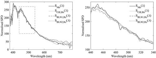
As anticipated, the localized reconstruction procedure outperformed the widely used CIE procedure in all analyses regarding accuracy. However, one unanticipated finding was that the higher accuracy in reconstruction had no major influence on the NIF assessment, or, as a matter of fact, on any application weighted with any of the five α-opic functions. Moreover, contrary to expectations, for $T_{cp}$ greater than 25,000 K, the CIE procedure outperformed BLN₂ for melanopic responses. As depicted in Fig. 17, although the BLN₂ localized method performed better on the whole in terms of mapping the measurement more accurately, when we zoom into the mid-wavelength range (440 nm – 540 nm), the localized BLN₂ reconstruction is less reflective of the measurement than the CIE reconstruction at high $T_{cp}$ (> 25,000 K). The above-mentioned predominantly overcast sky conditions in the localized modeling sampling could possibly explain the poorer reconstruction accuracy with high $T_{cp}$ (clear skies) for mid-range wavelengths.

Fig. 17. An overall (left) and detailed (right) display of a normalized measured spectral irradiance (-, gray, $S_{Me}\left(\lambda \right)$) retrieved on 30 March 2015, at 17:29:01 CEST, with a solar altitude of 18.09°, for sky patch 75 with $T_{cp}=76,294K$ as well as the corresponding reconstructions performed using the CIE method (-, $S_{CIE,Re}\left(\lambda \right)$); the BLN₁ method, using $x_{D,BLN},y_{D,BLN}$ (--,$S_{BLN1,Re}\left(\lambda \right)$); and the BLN₂ method, using $x_{D,BLN},y_{D,BLN}$ and components of the daylight distribution $S_{0,BLN}$, $S_{1,BLN}$, and $S_{2,BLN}$ (:, $S_{BLN2,Re}\left(\lambda \right)$).

The results of the application-related study do not support the thesis by Hernández-Andrés et al. (2001a, 2001b) asserting that more than three components are needed to reconstruct daylight SPD in the wavelength range of 380–780 nm for spectral purposes relating to humans’ visual and non-image forming systems. Our results largely corresponds to the findings of Tourasse and Dumortier (2015). To the best of our knowledge, no studies exist that address the importance of the accuracy of the reconstruction procedure on daytime NIF effects and that include an analysis of all five photoreceptors. Our findings, however, are in close agreement with the results presented by Bellia et al. (2020) relating the matching CIE illuminants to SPD measurements and evaluating the melanopic/photopic (M/P) ratio.

5.2. Study limitations

The generalizability of these results is subject to certain limitations. The primary shortcoming of this study is the single location for the validation data set. A separate but related problem is that the sample data underlying the CIE procedure as well as the data used to model the locally adapted procedure both represent temperate climates occurring in middle latitudes in the northern hemisphere. The generalizability of these results is therefore also limited to these latitudes. The results nevertheless are promising, and should be extended to include further data collection to determine how well the CIE procedure replicates daylight conditions at higher latitudes, to say nothing of the southern hemisphere. Another limitation is the omission of measurements during sunrise and sunset skies (solar altitude less than 15°). Also, the impact of haziness and the built environment on the spectral characteristics remains an open question. A future study will address this separately. Further analysis could be required to define whether global and patch measurements can be combined, and if direct sun measurements should be included. The conclusions drawn with regard to the sensitivity analysis refer only to NIF responses caused by ocular exposure to daylight and, accordingly, to the wavelength range between 380 nm and 780 nm. The reconstruction accuracy in the UV region lies outside the scope of the study, but a separate study would be worthwhile (Kobayashi et al. 1997). The NIF analysis was performed spectrally resolved, and the percent error was determined for eight $T_{cp}$ ranges selected based on Robertson (1968). For other applications with deviating action spectra, further analysis using a higher spectral resolution might be necessary.

6. Conclusions

This paper has presented a structured assessment and comparative analysis of the accuracy levels of SPD daylight reconstruction procedures, and to furthermore contextualizing the results in relation to NIF responses during daytime. This work showed that using a large and homogeneous data set to set up a localized reconstruction model is worthwhile, as 99.72% of the reconstructed SPD were colorimetrically and photometrically “accurate,” compared to only 95.97% using the CIE reconstruction method. However, only adapting the existing CIE reconstruction procedure by adopting a local daylight locus (in our case, Berlin) failed to result in more accurate reconstructed SPDs. Instead, it was necessary to modify the procedure with local components and weighting factors, all created with a refinement of the wavelength step size to 1 nm, to increase accuracy. Localized methods showed increased accuracy for summer and winter, for overcast and clear sky conditions, and for the $T_{cp}$ range from 4000 K to 25,000 K. For $T_{cp}$ beyond 25,000 K, the local Berlin method was comparable to the CIE method. From a practical point of view, the results showed that the local reconstruction procedure in Berlin was not necessary when it comes to evaluating NIF effects during the day at times when the solar altitude is above 15°. Even though the Berlin reconstruction procedure has a higher proportion of “good” and “accurate” reconstructions, this was not reflected in the accuracy of the NIF efficacy. Nevertheless, the results show that the NIF efficacies determined using SPDs – regardless of the reconstruction method – differed only minimally from the NIF efficacies determined using actual measurements.

The results presented here are significant in at least two major respects. First, the most significant general result to emerge is that the CIE reconstruction procedure could still be applicable in the context of NIF and that it is possible that no local adjustments are even necessary. In practical terms, this means that this procedure could be used to weight SPDs derived from measured $T_{cp}$ with the α-opic action spectra to assess NIF responses and therefore simplify measurement and representation systems. However, from a scientific point of view, the results support arguments in favor of a new worldwide procedure, since, as mentioned above, the CIE daylight locus is based on limited sampling data and was visually determined. With the growing possibilities of collecting and processing massive data sets and access to spatially resolved measurements, it would be worthwhile to update and scientifically substantiate the method with complementary data. Second, the localized procedure proved that $x_D$ can be derived seamlessly from $T_{cp}$. This has significant implications for computer simulations, as the two different $x_D$ functions currently employed by the CIE produce a discontinuity in the data at 7000 K. Given the growing importance of NIF effects in planning as well as the very limited access to spatially and spectrally resolved daylight SPD data, the results of this study corroborate the hypothesis that low-cost and widely accessible sensors and the representation of spectral properties with a single value, $T_{cp}$, can be used for NIF purposes.

Nomenclature

BLN1	=	Locally adjusted reconstruction method using Berlin daylight locus
BLN2	=	Locally adjusted reconstruction method using Berlin daylight locus and Berlin components
CIE	=	Commission Internationale de l’Éclairage
$\mathrm{G}\mathrm{F}\mathrm{C}$	=	Goodness-of-Fit Coefficient
$K_{\alpha ,v,Re}$	=	α-opic efficacy of luminous radiation (α-opic ELR)
${\mathrm{M}}_1,$ ${\mathrm{M}}_2$	=	Weighting factors
$\mathrm{M}\mathrm{A}\mathrm{P}{\mathrm{E}}_{\alpha }$	=	Mean absolute percentage error for α-opic quantities
$\mathrm{M}\mathrm{P}{\mathrm{E}}_{\alpha }$	=	Mean percentage error for α-opic quantities
NIF	=	Non-image forming
$\mathrm{R}\mathrm{M}\mathrm{S}\mathrm{P}{\mathrm{E}}_{\alpha }$	=	Root mean square percentage error for α-opic quantities
PCA	=	Principal component analysis
$S_i\left(\lambda \right)$	=	PCA components
$S_{Me}\left(\lambda \right)$	=	Measured spectral power distribution
$S_{Re}\left(\lambda \right)$	=	Reconstructed spectral power distribution
SPD	=	Spectral power distribution
$T_{cp}$	=	Correlated color temperature
x$,y$	=	Chromaticity coordinates
$x_D,y_D$	=	Daylight chromaticities, daylight locus

Acknowledgments

The authors would like to thank Eric Rockstädt, Lukas Liegener, Dimitri Belostotski, and Frederic Rudawski for their valuable support in programming.

Disclosure statement

No potential conflict of interest was reported by the author(s).

Supplementary material

Supplemental data for this article can be accessed on the publisher’s website.

Additional information

Funding

The authors have disclosed receipt of the following financial support for the research, authorship, and/or publication of this article: Aicha Diakite-Kortlever received a fellowship by the Velux Foundation (grant number 1087: “Development and Application of Spectral Sky Models in Urban Planning”).

References

- Aydinli S, Behrens K, Masuch J, Riecke W. 2016. Die Entwicklung der atmosphärischen Trübung in Deutschland. Konsequenzen für die Solarstrahlung. HLH. 02:21–25.
- Bellia L, Błaszczak U, Fragliasso F, Gryko L. 2020. Matching CIE illuminants to measured spectral power distributions: a method to evaluate non-visual potential of daylight in two European cities. Solar Energy. 208:830–858.
- Chain C. 2004. Caractérisation spectrale et directionnelle de la lumière naturelle: application à l Éclairage des Bâtiments. Vaulx-en-Velin (France): ENTPE, Laboratoire des Sciences de l’Habitat, Département Génie Civil et Bâtiment.
- CIE. 1994. Guide to recommended practice of daylight measurement. Vienna (Austria): CIE.
- CIE. 2003. Spatial distribution of daylight – CIE standard general sky. Vienna (Austria): CIE.
- CIE. 2018a. CIE system for metrology of optical radiation for ipRGC-influenced responses to light. Vienna: International Commission on Illumination.
- CIE. 2018b. Colorimetry. 4th ed. Vienna (Austria): CIE.
- Condit HR, Grum F. 1964. Spectral energy distribution of daylight*. J Opt Soc Am. 54(7):937.
- Diakite AK, and Knoop M. 2019. A data-driven colorimetric analysis of the CIE standard general skies. Proceedings of the 29th Quadrennial Session of the CIE Washington (USA). p. 353–62.
- Diakite AK, Weber N, Knoop M, and Rockstädt E. 2018. Optimierung des Verfahrens zur Rekonstruktion von Tageslichtspektren aus Farbörter auf dem Daylight Locus. Proceedings of LICHT Davos (CH).
- Diakite-Kortlever AK, Knoop M. 2021. Forecast accuracy of existing luminance-related spectral sky models and their practical implications for the assessment of the non-image-forming effectiveness of daylight. Light Res Technol. 147715352098226. doi:10.1177/1477153520982265
- Dixon ER. 1978. Spectral distribution of Australian daylight. J Opt Soc Am. 68(4):437.
- Henderson ST. 1977. Daylight and its spectrum. 2 ed. Bristol: Hilger. p. 349 s.
- Henderson ST, Hodgkiss D. 1963. The spectral energy distribution of daylight. Br J Appl Phys. 14(3):125–131.
- Hernández-Andrés J, Lee RL, Romero J. 1999. Calculating correlated color temperatures across the entire gamut of daylight and skylight chromaticities. Appl Opt. 38(27):5703–5709.
- Hernández-Andrés J, Nieves JL, Valero EM, Romero J. 2004. Spectral-daylight recovery by use of only a few sensors. J Opt Soc Am A. 21(1):13–23.
- Hernández-Andrés J, Romero J, García-Beltrán A, Nieves JL. 1998. Testing linear models on spectral daylight measurements. Appl Opt. 37(6):971–977.
- Hernández-Andrés J, Romero J, Lee RL,JR. 2001a. Colorimetric and spectroradiometric characteristics of narrow-field-of-view clear skylight in Granada, Spain. J Opt Soc Am A. 18(2):412–420.
- Hernández-Andrés J, Romero J, Nieves JL, Lee R. 2001b. Color and spectral analysis of daylight in Southern Europe. J Opt Soc Am A. 18(6):1325–1335.
- Hosek L, Wilkie A. 2012. An analytic model for full spectral sky-dome radiance. ACM Trans Graph. 31(4):1–9.
- Inanici M. 2019. Tri-stimulus color accuracy in image-based sky models: simulating the impact of color distributions throughout the sky dome on daylit interiors with different orientations. Proceedings of the 16th IBPSA Rome (Italy). p. 1052–59.
- Judd DB, MacAdam DL, Wyszecki G, Budde HW, Condit HR, Henderson ST, Simonds JL. 1964. Spectral distribution of typical daylight as a function of correlated color temperature. J Opt Soc Am. 54(8):1031.
- Kawakami G, Ando I, Ikemori T. 1965. Study of daylight (II). J Illum Eng Inst Japan. 49(9):521–526.
- Knoop M, Abdelmageed AA, Luo T, Weber N, Diakite AK. 2017. Spatially resolved spectral sky daylight measurement data: methods of collection, evaluation and representation. Proceedings of the CIE 2017 Midterm Meeting, 23 to 25 October 2017, Jeju, Republic of Korea. p. 1036–46.
- Knoop M, Broszio K, Diakite A, Liedtke C, Niedling M, Rothert I, Rudawski F, Weber N. 2019a. Methods to describe and measure lighting conditions in experiments on non-image-forming aspects. LEUKOS. 15(2–3):163–179.
- Knoop M, Diakite A, Rudawski F. 2015. Methodology to create spectral sky models to enable the inclusion of colorimetric characteristics of daylight in research and design. Proceedings of the 28th Session of the CIE, 28 June to 4 July 2015, Manchester, United. p. 564–73.
- Knoop M, Stefani O, Bueno B, Matusiak B, Hobday R, Wirz-Justice A, Martiny K, Kantermann T, Aarts MPJ, Zemmouri N, Appelt S, and Norton B . 2020. Daylight: what makes the difference? Light Res Technol. 52(3):423–442.
- Knoop M, Weber N, Diakite AK. 2019b. Approach to analyse seasonal and geographical variations in daylight illuminants. Proceedings of the 29th CIE SESSION, 14 – 22 June 2019, Washington D.C., USA. p. 195–204.
- Kobav MB, Bizjak G, Dumortier D. 2013. Characterization of sky scanner measurements based on CIE and ISO standard CIE S 011/2003. Light Res Technol. 45(4):504–512.
- Kobayashi K, Ikemori T. 1993. Color of daylight in snowy region. J Illuminating Eng Institute of Japan. 77(11):693–695.
- Kobayashi K, Ikemori T, Kawakami G. 1997. Spectral distribution of north sky daylight - measurement and reconstitution of spectral distirbution. J Illuminating Eng Institute of Japan. 81(11):983–989.
- Kobayashi K, Kawakami G, Okuma Y, Ikemori T. 1996. Spectral distributions of north sky daylight at Atsugi. J Illuminating Eng Institute of Japan. 80(8):550–553.
- Lucas RJ, Peirson SN, Berson DM, Brown TM, Cooper HM, Czeisler CA, Figueiro MG, Gamlin PD, Lockley SW, O’Hagan JB, et al. 2014. Measuring and using light in the melanopsin age. Trends Neurosci. 37(1):1–9.
- McCamy CS. 1992. Correlated color temperature as an explicit function of chromaticity coordinates. Color Res Appl. 17(2):142–144.
- Münch M, Wirz-Justice A, Brown SA, Kantermann T, Martiny K, Stefani O, Vetter C, Wright Jr. KP, Wulff K, and Skene DJ . 2020. The role of daylight for humans: gaps in current knowledge. Clocks Sleep. 2(1):61–85.
- Nayatani Y, Wyszecki G. 1963. Color of daylight from North Sky. J Opt Soc Am. 53(5):626.
- Nieves JL, Valero EM, Nascimento SMC, Hernández-Andrés J, Romero J. 2005. Multispectral synthesis of daylight using a commercial digital CCD camera. Appl Opt. 44(27):5696–5703.
- Riechelmann S, Schrempf M, Seckmeyer G. 2013. Simultaneous measurement of spectral sky radiance by a non-scanning multidirectional spectroradiometer (MUDIS). Meas Sci Technol. 24(12):12.
- Robertson AR. 1968. Computation of correlated color temperature and distribution temperature. J Opt Soc Am. 58(11):1528.
- Romero J, García-Beltrán A, Hernández-Andrés J. 1997. Linear bases for representation of natural and artificial illuminants. J Opt Soc Am A. 14(5):1007.
- Rossotti H. 1983. Colour. Princeton (NJ): Princeton University Press. p. 239.
- Rusnák A. 2014. Meranie a hodnotenie spektrálnych charakteristík slnečného žiarenia. [Measurements and evaluation of spectral sun radiation characteristics, Translation by Dr. Darula]. Bratislava (Slovenia): Slovenská Technická Univerzita v Bratislave.
- Sastri V, Das SR. 1968. Typical spectral distributions and color for tropical daylight. J Opt Soc Am. 58(3):391–398.
- Schlangen LJM, Price LLA. 2021. The lighting environment, its metrology, and non-visual responses. Front Neurol. 12:624861.
- Sekine S. 1989. Spectral distributions of clear sky light and their chromaticities. J Illuminating Eng Institute of Japan. 73(2):39–45.
- Sekine S. 1991. Spectral distributions of clear sky light and their chromaticities. J Light & Vis Env. 15(1):23–32.
- Simonds JL. 1963. Application of characteristic vector analysis to photographic and optical response data*. J Opt Soc Am. 53(8):968.
- Souman JL, Tinga AM, Te Pas SF, van Ee R, Vlaskamp BNS. 2018. Acute alerting effects of light: a systematic literature review. Behav Brain Res. 337:228–239.
- Takagi A, Takaoka H, Oshima T, Ogata Y. 1990. Accurate rendering technique based on colorimetric conception. ACM SIGGRAPH Computer Graphics. 24(4):263–272.
- Tarrant AWS. 1968. The spectral power distribution of daylight. Light Res Technol. 33(3 IEStrans):75–82.
- Tohsing K, Schrempf M, Riechelmann S, Seckmeyer G. 2014. Validation of spectral sky radiance derived from all-sky camera images – a case study. Atmos Meas Tech. 7(7):2137–2146.
- Tourasse G, and Dumortier D 2015. Long term measurements of sky spectral irradiances and validation of CIE daylight illuminants. Proceedings CIE Session 2015 Manchester (UK), Vol. 1, Part 1. p. 708–717.
- Tregenza PR. 1987. Subdivision of the sky hemisphere for luminance measurements. Light Res Technol. 19(1):13–14.
- Tregenza PR. 2004. Analysing sky luminance scans to obtain frequency distributions of CIE standard general skies. Light Res Technol. 36(4):271–281.
- Weber N, Knoop M, and Völker S. 2016. Adaptive tageslichtabhängige Lichtsteuerung für nicht-visuell wirksame Beleuchtung. Proceedings of LICHT 2016 Karlsruhe (D). p. 229–234.
- Winch GT, Boshoff MC, Kok CJ, Du Toit AG. 1966. Spectroradiometric and colorimetric characteristics of daylight in the Southern Hemisphere: pretoria, South Africa. J Opt Soc Am. 56(4):456–464.
- Wirz-Justice A, Skene DJ, Münch M. 2020. The relevance of daylight for humans. Biochem Pharmacol. 114304.
- Wright H. 1965. Daylight and correlated color temperature. J Opt Soc Am. 55(6):741.
- Yatsuzuka H, Uetani Y. 2013. Measurement of the all sky spectral radiance distribution using a digital camera with a fisheye lens. Nihon Kenchiku Gakkai Kankyokei Ronbunshu. 78(690):623–629.
- Yatsuzuka H, Uetani Y. 2014. Estimation of the spectral radiance of a sky element using principal component analysis. Nihon Kenchiku Gakkai Kankyokei Ronbunshu. 79(697):227–232.
- Zeitzer JM. 2018. When is a proxy not a proxy? The foibles of studying non-image forming light. J Physiol. 596(11):2029–2030.