A Grid in Perspective for Road Lighting Calculations

ABSTRACT

In road lighting, calculations are made within the rectangular CIE grid while measurements conducted with Imaging Luminance Measurement Devices (ILMD) have a trapezoidal shape. We propose to build a grid that takes the observer’s perspective into account by projecting ellipses of adjustable dimensions than can match human vision or ILMD angular aperture and allow direct comparison with luminance images. Lighting standard criteria definitions remain unchanged and values of average luminance and longitudinal uniformity are equivalent. However, as the grid in perspective describes more finely the luminance distribution, the overall uniformity is lower than in the classical grid but more representative of observer’s perception. We present in detail our approach, give the corresponding code, expose calculations performed with this new grid and show an example of direct comparison between calculations and measurements.

KEYWORDS:

• Road lighting quality
• calculation grid

1. Introduction

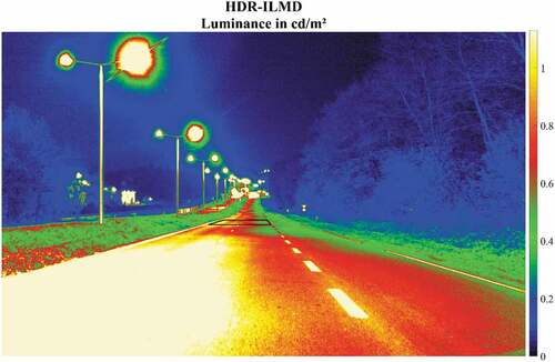
The design of road lighting installations is performed according to the specifications of CIE documents and relevant standards (ANSI/IESNA, 2000; CEN 2015; CIE 2019). To calculate luminance-based quality criteria, a rectangular grid of the relevant area has to be defined. There are usually three transversal points and a minimum of ten longitudinal points per traffic lane, i.e. typically 60 points for two lanes (Fig. 1). This standard methodology is efficient, very pragmatic for on-site punctual measurements and does not need advanced calculation tools. For more than 60 years, manual measurements were conducted by luxmeters, then replaced by punctual luminance meters and recently by Imaging Luminance Measurement Devices (ILMD’s). Nowadays in road lighting design, ILMD’s are able to produce experimental luminance maps like the one in Fig. 2. Their angular resolution can be much finer than that of the human eye (Buschmann et al. 2017; Greffier et al. 2019; Rossi et al. 2017). These on-site images are often compared with calculations obtained by common lighting calculation software (Radiance, Dialux, Relux) that still use the standard grid.

Fig. 1. Standard grid definition.

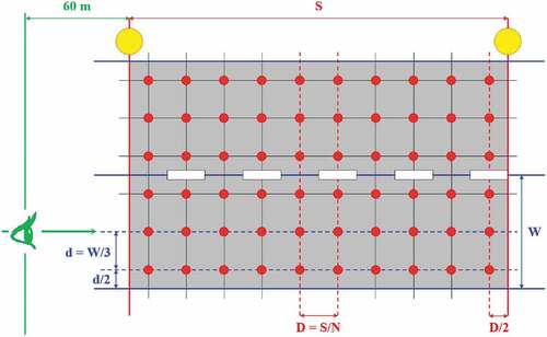
Fig. 2. Luminance measurement map from the standard observer’s perspective.

Discrepancies are often observed between simulations and experimental measurements regarding the quality criteria (average luminance, overall and longitudinal uniformities) and luminance distributions. These deviations may be due to various factors:

• uncertainties on light sources distribution and power,

• the use of a standard r-table in calculations instead of a measured r-table,

• planarity defaults,

• uncertainty of the luminance-measuring device,

• methodology of exploitation of the experimental luminance measurement.

In this paper, we will address this last possible source of discrepancy. Having a common exploitation of ILMD is a first step, available to all and easy to implement.

On the one hand, the camera provides a perspective image of the measured area, which has a trapezoidal shape. On the other hand, the calculations are carried out on a rectangular grid defined by the CIE. To match the ILMD experimental results and the calculations with the standard CIE 6 × 10 grid, several methodologies are possible, like:

1. Stretching the trapezoidal shape to transform it in a rectangular one. Then, the grid points are calculated by a rectangular shape, or

2. Projecting the grid points in the ILMD trapezoidal shape.

The method a. involves transforming the imaged field from a trapezoidal shape to a rectangular one (Buschmann et al. 2020). This mathematical transformation is called a rectification and requires interpolations that have an impact on the measurements (Boucher et al. 2021).

The method b. does not transform the measured field but needs to define the grid points according to the parameters as height, line of sight, pixel size, focal length. It is finally a way to take into account the observer’s perspective at the price of many geometrical calculations.

The final step, common for both methods, is to average luminances within areas of dimensions about 2’x20’ (arcminutes) centered on the grid points. These dimensions are a requirement of (CIE 2011) but its justification is related to (AFNOR 2006) for tunnel lighting that does not provide additional justification nor references. Whatever the method, the fine angular resolution of ILMD is lost because the luminance distribution is finally described by only 6 × 10 values.

In this paper, we expose a method of direct comparison between experimental luminance image and calculation. This method will not resolve the discrepancies often observed due to lack of knowledge of some parameters (real source power, exact source tilt, planarity default, road surface r-table, …). But our aim is to propose and diffuse a method that do not induce deviations due to the mathematical process. Therefore, in our approach, the measured luminance map is not transformed to match a calculation grid, but conversely adapts the calculation to the measurement.

The general principle is the following. Instead of the classic grid, a grid based on observer’s perspective and a given angular aperture is used.

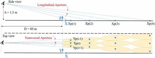
• The positions of the grid points are defined as the centers of ellipses projected from the observer’s position with given angular apertures in the longitudinal direction and in the transverse direction (Fig. 3). Angular apertures can be chosen to simulate the observer’s vision, then ellipses represent the retinal cells projection on the road surface. Whether they are known, apertures can fit the ILMD ones. For ILMD measurements, (CEN 2015) recommends an angular aperture in the range [1’, 2’].

  Fig. 3. Ellipses projection from observer’s eye.

  

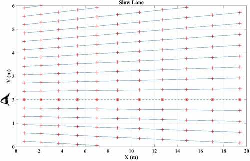
• Taking observer’s position as a reference, the first line of the grid is constructed by ellipses projection in front of the observer. It corresponds to the center of the driving lane. This first line (star markers in Fig. 4) is used to the longitudinal uniformity calculation as defined in standards.

  Fig. 4. Points coordinates within the grid in perspective (ApL = 2’, ApT = 20’).

  

• The whole grid is generated adding ellipses next to the first line according to the ellipses width. As the ellipses width increases with distance, the grid owns more ellipses at the beginning of the mesh than at the end, translating the perspective view.

The grid in perspective owns some hundreds of points describing more finely the luminance distribution than the classical grid. It adapts the calculation to the field of view and generates a trapezoidal grid more convenient to fit ILMD images. Moreover, the three classical road lighting criteria definitions are unchanged.

Our goal here is to describe in detail our approach and to give the corresponding code so that it becomes available to all. We also present results on calculations under several lighting situations and an example of comparison between measurement and calculation.

2. Perspective grid construction

In the following we describe step by step the construction of the grid. All the variables implied and the Matlab® code lines are explained. The entire code is available in Appendix A.

First we need to define some scene parameters: the road width, the spacing between two luminaires, the observer’s position and the apertures of ellipses. In this example, the axis origin states at 60 m from the observer (see Fig. 3) and angular apertures are fixed to 2’.

%variables definition Spacing = 20 ; % spacing between two luminaires in mWr = 6; % road width in mObs.X = -60 ; % longitudinal observer’s position in mObs.Y = [4 2] ; % transversal observer’s positions in mObs.Z = 1.5 ; % observer’s eye height in mApL = 2/60 ; % Longitudinal Aperture in degreeApT = 2/60 ; % Transversal Aperture in degree

First, we calculate the abscissas of ellipses’ centers. The first center abscissa Xp(1) is shifted from the 60 m line by a half of the longitudinal aperture. A bit of trigonometry leads to the following expression:

%abscissas of ellipses’ centresXp = Obs.Z/tand(atand(Obs.Z/abs(Obs.X))-1/2*ApL) ; % first centre abscissa

Then abscissas Xp(i) are calculated recursively with a decreasing projection angle substracting the longitudinal aperture each time. Results are stored in a vector Xp while the calculated center stands in the calculation area.

while Xp(end)<(Spacing + abs(Obs.X)) % abscissas into the calculation area Xp = [Xp ; Obs.Z/tand(atand(Obs.Z/Xp(end))-ApL)] ; end Xp = Xp(1:end-1) ;% delete the last value outside the area

Output vectors are instantiated. They correspond to centers’ coordinates for two separate observer’s positions, one in the center of the fast lane and the other in the center of the slow lane.

Xp_FL = [] ; % Abscissas of points for fast lane observer’s positionYp_FL = [] ; % Ordinates of points for fast lane observer’s positionXp_SL = [] ; % Abscissas of points for slow lane observer’s positionYp_SL = [] ; % Ordinates of points for slow lane observer’s position

Ordinates of ellipses’ centers can now be calculated for each abscissa. As they depend on observer’s transverse position, the procedure for the fast lane will be repeated for the slow lane (given in Appendix A). The first ordinate corresponds to the center of the given lane. A counter is also initialized to keep track of the number of centers on each side of the center of the lane. It will be used to construct a mask representing the grid seen by the observer.

%ordinates of ellipses’ centres for x = 1:length(Xp)% fast laneYp = Obs.Y(1) ;% first centre ordinatec1=-1;% count centres on the left side of the first centre% (seen from the observer)

Ordinates Yp(i) are calculated recursively from the first center adding the transversal aperture each time. They stand on the left side of the first center seen from the observer. Results are stored in a vector Yp in descending order while the calculated ordinate is inside the road width.

while Yp(1)<Wr % ordinates into the road widthYp = [Xp(x)*tand(atand(Yp(1)/Xp(x))+ApT) ; Yp] ;c1=c1+1;endYp = Yp(2:end) ;% delete last value outside the road width

Then ordinates Yp(i) corresponding to the right side of the first center are calculated by subtracting the transversal aperture each time.

c2=-1;% count centres on the right side of the first centre (seen from the observer)while Yp(end)>0 % ordinates into the road widthYp = [Yp ; Xp(x)*tand(atand(Yp(end)/Xp(x))-ApT)] ;c2=c2+1;endYp = Yp(1:end-1) ; % delete last value outside the road width

At this point, all ordinates have been calculated for each abscissa. They can be stored in the output vectors taking care of vectors dimensions and of the axis origin.

Xp_FL = [Xp_FL ; Xp(x)*ones(length(Yp),1)+Obs.X] ;Yp_FL = [Yp_FL ; Yp] ;

Besides the grid points coordinates used for further calculations, an image (in pixels) seen by the observer is also constructed. It will allow a direct comparison with experimental measurements. The image is initialized once the first row of centers is calculated. The image is defined as an array of dimensions: number of abscissas by number of ordinates at the first abscissa. As the number of ellipses decreases with distance by the perspective effect, the image will finally look like a trapezoid surrounded by zeros.

if x==1% image seen from observer’s position center_lane_FL=c1+1; % index of central rowMask_FL=zeros(length(Xp),length(Yp),‘logical’); % mask initialisationendMask_FL(length(Xp)-x+1,center_lane_FL-c1:center_lane_FL+c2)=1; %fill image at given indices

The same procedure is repeated for the slow lane observer’s position.

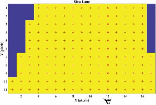
Calculations can now be done at (Xp_SL,Yp_SL) positions for an observer in slow lane and at (Xp_FL,Yp_FL) positions for an observer in fast lane. Figure 4 presents results of previous calculations for the slow lane observer’s position (with ApT = 20’ to be drawable). Star markers represent the line in front of the observer.

Mask_SL and Mask_FL matrices can be filled with calculated luminances to compare with ILMD images. Note that the longitunal and transverse aperture parameters, ApL and ApT, can be adjusted to exactly match the imaging system if needed. Figure 5 shows the image Mask_SL with ApL = 2’ and ApT = 20’ where (Xp_SL, Yp_SL) crosses are superimposed.

Fig. 5. Mask of the grid in perspective seen by the observer (ApL = 2’, ApT = 20’).

3. Calculations with the grid in perspective

To assess the impact of using the grid in perspective instead of the classical CIE one, simulations were conducted with both approach on 10 different lighting situations. The seven CIE situations proposed in (CIE 2019) with standard r-table R3 (CIE 2001) and three French experimental situations evaluated during the Lumiroute® experiment (Muzet et al. 2019) with LED or Metal Halide luminaires and experimental r-tables obtained on site with Coluroute device (Muzet et al. 2008). The parameters of the 10 lighting situations are given in Appendix B.

All calculations are made with Ecl_R, a lighting calculation engine developed by Cerema (Greffier et al. 2021).

For both approaches, the lighting quality criteria of (CEN 2016) were performed:

• The average luminance is calculated as the arithmetic mean of the luminances obtained at the grid points.

• The overall uniformity, Uo, is calculated as the ratio of the lowest luminance to the average luminance in the field of calculation.

• The longitudinal uniformity, Ul, is calculated as the ratio of the lowest to the highest luminance in the longitudinal direction along the center-line of each lane. The observer’s position should be in line with the row of calculation points.

All the results are presented in the Table 1. The deviations in percentage between the two grids are computed using (X_{perspective –} X_classical)/X_classical * 100, where X stands for average luminance and uniformities. As expected, the average luminance varies very little between the classical and perspective grids. Indeed, the average value is not very sensitive to the number of calculation points. The longitudinal uniformity is also not very sensitive to the grid change as about the same number of longitudinal points are used. On the other hand, the overall uniformity is always higher with the classical grid. The perspective grid containing a larger number of calculation points, the luminance distribution is analyzed more finely than with 60 points. This explains why the extreme values (min and max) are different and lead to lower overall uniformities. If angular apertures are chosen to simulate the vision, this overall uniformity seems more representative of the observer’s perception because it is closer to the eye angular resolution.

Table 1. Lighting quality criteria calculations with classical and perspective grid.

		Classical Grid		Grid in Perspective		Deviation
		fast lane	slow lane	fast lane	slow lane	fast lane	slow lane
Situation CIE 1	Laverage	0.26	0.26	0.25	0.25	−4%	−4%
	Uo	0.14	0.15	0.12	0.12	−16%	−19%
	Ul	0.56	0.64	0.55	0.64	−2%	1%
Situation CIE 2	Laverage	0.26	0.26	0.26	0.26	−2%	−2%
	Uo	0.32	0.35	0.25	0.26	−23%	−26%
	Ul	0.33	0.33	0.34	0.34	3%	1%
Situation CIE 3	Laverage	0.55	0.60	0.52	0.58	−5%	−4%
	Uo	0.52	0.54	0.5	0.51	−5%	−6%
	Ul	0.68	0.70	0.65	0.71	−3%	2%
Situation CIE 4	Laverage	0.88	0.87	0.87	0.83	−1%	−4%
	Uo	0.54	0.51	0.47	0.46	−13%	−10%
	Ul	0.53	0.53	0.53	0.53	0%	1%
Situation CIE 5	Laverage	0.44	0.41	0.42	0.39	−3%	−3%
	Uo	0.45	0.67	0.43	0.63	−5%	−6%
	Ul	0.79	0.75	0.79	0.74	0%	−2%
Situation CIE 6	Laverage	1.17	1.31	1.09	1.24	−7%	−5%
	Uo	0.49	0.49	0.47	0.46	−3%	−6%
	Ul	0.62	0.72	0.61	0.72	−1%	0%
Situation CIE 7	Laverage	0.53	0.58	0.53	0.58	−1%	0%
	Uo	0.45	0.46	0.41	0.41	−8%	−11%
	Ul	0.84	0.91	0.82	0.88	−2%	−3%
LUMIROUTE® 1	Laverage	0.89	0.95	0.88	0.94	−1%	0%
	Uo	0.56	0.57	0.49	0.48	−12%	−14%
	Ul	0.84	0.79	0.85	0.77	1%	−2%
LUMIROUTE® 2	Laverage	1.21	1.28	1.2	1.26	−1%	−1%
	Uo	0.61	0.62	0.54	0.54	−11%	−13%
	Ul	0.82	0.82	0.82	0.79	1%	−3%
LUMIROUTE® 4	Laverage	0.71	0.78	0.70	0.77	−1%	−1%
	Uo	0.66	0.66	0.58	0.56	−13%	−15%
	Ul	0.77	0.78	0.73	0.77	−4%	−1%

4. Measurement vs calculation

A comparison of simulated luminance and measurement with ILMD has been conducted on the test case LUMIROUTE® 4. Luminaires stand at a height of 9 m with a spacing of 29 m. The road width is 5.7 m. The road reflection characteristics have been measured by taking drill core samples and measuring the r-table in laboratory according to (CIE 2001). Road surface exhibits a Q0 = 0.066 and S1 = 1.10 and the corresponding r-table is used for the following ECL_R calculations.

Image luminance measurements were conducted using an HDR-ILMD (Boucher et al. 2017) based on four CMOS cameras to provide a wide range of luminance. The standard observer’s position according to (CIE 2019) was used and luminance maps were recorded with the above mentioned setup. The focal length of the imaging system is 12.5 mm and the pixel pitch of the sensor is 5.86 μm, thus the pixel angular aperture is 1.5’ (averaged over the whole sensor area) and the measurement field is imaged by 18 × 226 pixels (black trapeze in Fig. 2).

The method b. is first applied in averaging the luminance over 1.5’ × 20’ (i.e. 1 × 13 pixels) around each grid point. Figure 6 (left) presents results of method b. applied on the ILMD image. Figure 6 (right) presents result of calculation.

Fig. 6. Measured grid by method b. (left) and calculated grid (right) for the 60 CIE points.

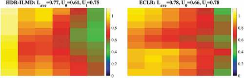
In this test case, for the classical 6 × 10 grid, the measured and calculated road lighting quality criteria are in very good agreement, with a difference of 1.3% for luminance and a maximum difference of 7.6% for overall uniformity. Since all the parameters (light sources, scene geometry, road surface and measured area) have been carefully measured, it explains why calculations are able to reproduce measurements. It should be noted that this level of knowledge is rarely achieved in operational conditions.

Applying the perspective method with angular apertures, ApT and ApL equal to 1.5’, the grid contains 215 points (ellipse centers) at 60 m in transverse direction, 148 points at 89 m and 19 points in longitudinal. Then the image dimension is 19 × 215 pixels with a trapezoidal luminance map surrounded by zeros (see Fig. 7). This dimension is near but not exactly the experimental image (18 × 226). So the measured image is resized to fit exactly the calculation. We have verified that there is no incidence on results (up to third digit). Figure 7 (left) presents the ILMD trapezoidal area of Fig. 2 resized to fit exactly the calculated grid size. Figure 7 (right) presents result of calculation with ApT and ApL equal to 1.5’.

Fig. 7. Measured grid (left) and calculated grid (right) using the grid in perspective.

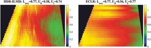
For the perspective method with a large number of measurement considered (3444 points), the measured and calculated road lighting quality criteria are also in very good agreement, with a maximum difference of 4%. One minor drawback of this method is illustrated in Fig.7 (left): it includes the central marking whereas it is not present in the CIE grid. Here, markings are imaged by 30 pixels representing less than 1% of the imaged area and their influence can be considered negligible. If it is not the case, markings should be removed.

Whatever the number of points considered, average luminance and longitudinal uniformity are not sensitive to the grid change. However the overall uniformity decreases with the perspective grid as the luminance distribution is much more finely described (but remains over the standard threshold of U0 ≥0.4).

We have shown with this example that the CIE lighting criteria are still consistent between calculation and measurement with the perspective method. Finally, there is no more need to project points in an image frame. Benefits of the perspective grid are to not induce errors due to a stretching of the measured data (to fit a rectangle from a trapeze) and to allow a direct comparison as the calculation fits exactly the measured image.

5. Conclusion

The comparison of luminance maps cannot be made directly between experiments and calculations: on the one hand, the camera provides a perspective image of the area to be measured, on the other hand, the calculations are carried out on a rectangular grid defined by the CIE. To avoid the drawbacks of a comparison between trapezoidal measurements and rectangular calculations, we propose to build a grid that takes the observer’s perspective into account by projecting ellipses of adjustable dimensions than can match human vision or imaging system angular aperture and allow direct comparison with images provided by an ILMD.

In this paper, we present both the methodology and a software implementation, providing the code in appendix.

To test the implementation, lighting quality criteria calculations have been carried out using the 60 points CIE grid and our approach for ten situations: seven CIE situations and three experimental ones. Whatever the methodology, the lighting standard criteria definitions remain unchanged and we have shown that the values of average luminance and longitudinal uniformity are equivalent. The luminance distribution is more finely described using more calculation points, thus calculated and measured overall uniformity tends to decrease but it is more representative of the driver’s perception. A trapezoidal mask is also generated and is used to fit ILMD images.

The example of the comparison between calculation and measurement shows the advantages of the perspective grid. Increasing the resolution could allow other quality criteria to be considered. For example, the standard deviation of the luminance distribution could be used to represent a more representative overall uniformity than the ratio of two values. Gradient calculations in the longitudinal and transverse directions could also become uniformity criteria in these dimensions. They might be more representative of visual comfort than the track axis alone. This work now needs to be consolidated by multiple comparisons between calculations and measurements to confirm the trends. We hope that researchers in the field will use this new grid to explore its potential.

Disclosure statement

No potential conflict of interest was reported by the authors.

Additional information

Funding

This work was supported by the Cerema “Tremplin Europe & International” under Grant Savaphor-2020.

APPENDICES Appendix A.

Grid calculation code

%variables definition

Spacing = 20 ; % spacing between two luminaires in m

Wr = 6; % road width in m

Obs.X = -60 ; % longitudinal observer’s position in m

Obs.Y = [4 2] ; % transversal observer’s positions in m

Obs.Z = 1.5 ; % observer’s eye height in m

ApL = 2/60 ; % Longitudinal Aperture in degree

ApT = 2/60 ; % Transversal Aperture in degree

%abscissas of ellipses’ centres

Xp = Obs.Z/tand(atand(Obs.Z/abs(Obs.X))-1/2*ApL) ;% first centre abscissa

while Xp(end)<(Spacing + abs(Obs.X)) % abscissas into the calculation area

Xp = [Xp ; Obs.Z/tand(atand(Obs.Z/Xp(end))-ApL)] ;

end

Xp = Xp(1:end-1) ;% delete the last value outside the area

Xp_FL = [] ; % Abscissas of points for fast lane observer’s position

Yp_FL = [] ; % Ordinates of points for fast lane observer’s position

Xp_SL = [] ; % Abscissas of points for slow lane observer’s position

Yp_SL = [] ; % Ordinates of points for slow lane observer’s position

%ordinates of ellipses’ centres

for x = 1:length(Xp)

% fast lane

Yp = Obs.Y(1) ;% first centre ordinate

c1=-1;% count centres on the left side of the first centre % (seen from the observer)

while Yp(1)<Wr % ordinates into the road width

Yp = [Xp(x)*tand(atand(Yp(1)/Xp(x))+ApT) ; Yp] ;

c1=c1+1;

end

Yp = Yp(2:end) ;% delete last value outside the road width

c2=-1;% count centres on the right side of the first centre % (seen from the observer)

while Yp(end)>0 % ordinates into the road width

Yp = [Yp ; Xp(x)*tand(atand(Yp(end)/Xp(x))-ApT)] ;

c2=c2+1;

end

Yp = Yp(1:end-1) ; % delete last value outside the road width

Xp_FL = [Xp_FL ; Xp(x)*ones(length(Yp),1)+Obs.X] ;

Yp_FL = [Yp_FL ; Yp] ;

if x==1

% image seen from observer’s position

center_lane_FL=c1+1; % index of central row

Mask_FL=zeros(length(Xp),length(Yp),’logical’); % mask initialisation

end

Mask_FL(length(Xp)-x+1,center_lane_FL-c1:center_lane_FL+c2)=1; %fill image at given indices

% slow lane

Yp = Obs.Y(2) ; % first centre ordinate

c3=-1;% count centres on the left side of the first centre % (seen from the observer)

while Yp(1)<Wr

Yp = [Xp(x)*tand(atand(Yp(1)/Xp(x))+ApT) ; Yp] ;

c3=c3+1;

end

Yp = Yp(2:end) ; % delete last value outside the road width

c4=-1;% count centres on the right side of the first centre % (seen from the observer)

while Yp(end)>0

Yp = [Yp ; Xp(x)*tand(atand(Yp(end)/Xp(x))-ApT)] ;

c4=c4+1;

end

Yp = Yp(1:end-1) ; % delete last value outside the road width

Xp_SL = [Xp_SL ; Xp(x)*ones(length(Yp),1)+Obs.X] ;% abscissas coord.

Yp_SL = [Yp_SL ; Yp] ;% ordinates coord.

if x==1

% image seen from observer’s position

center_lane_SL=c3+1; % index of central row

Mask_SL=zeros(length(Xp),length(Yp),’logical’); % mask initialisation

end

Mask_SL(length(Xp)-x+1,center_lane_SL-c3:center_lane_SL+c4)=1; %fill image at given indices

end

Appendix B.

CIE and LUMIROUTE® Situations

Situation CIE 1

Table

Luminaire	Source Type	Fluo compact
	Photometry	Sit1.xls
	Height	4 m
	Spacing	20 m
	Overhang	2 m
	Tilt	0°
	Power	24 W
	Flux	1 800 lm
	Arrangement	Single-sided Left
	Maintenance Factor	0.8
Road	Surface	Standard R3
	Width	10 m
	Lanes	2
Observer	Observation angle	1°

Situation CIE 2

Table

Luminaire	Source Type	Fluo compact
	Photometry	Sit2.xls
	Height	4 m
	Spacing	20 m
	Overhang	2 m
	Tilt	0°
	Power	24 W
	Flux	1 800 lm
	Arrangement	Staggered
	Maintenance Factor	0.8
Road	Surface	Standard R3
	Width	10 m
	Lanes	2
Observer	Observation angle	1°

Situation CIE 3

Table

Luminaire	Source Type	High-pressure Sodium
	Photometry	Sit3.xls
	Height	10 m
	Spacing	45 m
	Overhang	0 m
	Tilt	5°
	Power	100 W
	Flux	10 500 lm
	Arrangement	Single-sided Left
	Maintenance Factor	0.8
Road	Surface	Standard R3
	Width	7.5 m
	Lanes	2
Observer	Observation angle	1°

Situation CIE 4

Table

Luminaire	Source Type	High-pressure Sodium
	Photometry	Sit4.xls
	Height	8 m
	Spacing	35 m
	Overhang	0 m
	Tilt	5°
	Power	100 W
	Flux	10 500 lm
	Arrangement	Staggered
	Maintenance Factor	0.8
Road	Surface	Standard R3
	Width	7 m
	Lanes	2
Observer	Observation angle	1°

Situation CIE 5

Table

Luminaire	Source Type	High-pressure Sodium
	Photometry	Sit5.xls
	Height	12 m
	Spacing	54 m
	Overhang	0 m
	Tilt	5°
	Power	100 W
	Flux	10 500 lm
	Arrangement	Opposite
	Maintenance Factor	0.8
Road	Surface	Standard R3
	Width	10.5 m
	Lanes	3
Observer	Observation angle	1°

Situation CIE 6

Table

Luminaire	Source Type	High-pressure Sodium
	Photometry	Sit6.xls
	Height	18 m
	Spacing	75 m
	Overhang	−2.25 m
	Tilt	5°
	Power	250 W
	Flux	32 000 lm
	Arrangement	Central
	Maintenance Factor	0.8
Road	Surface	Standard R3
	Width	7 m
	Lanes	2
Observer	Observation angle	1°

Situation CIE 7

Table

Luminaire	Source Type	High-pressure Sodium
	Photometry	Sit7.xls
	Height	10 m
	Spacing	40 m
	Overhang	0 m
	Tilt	5°
	Power	90 W
	Flux	13 000 lm
	Arrangement	Single-sided Left
	Maintenance Factor	0.8
Road	Surface	Standard R3
	Width	8 m
	Lanes	2
Observer	Observation angle	1°

Situation LUMIROUTE® 1

Table

Luminaire	Source Type	LED
	Photometry	Lumiroute1.xls
	Height	9 m
	Spacing	30 m
	Overhang	−0.62 m
	Tilt	0°
	Power	50 W
	Flux	3 500 lm
	Arrangement	Central
	Maintenance Factor	1
Road	Surface	S1Lumi1P1BrT36
	Width	6.5 m
	Lanes	2
Observer	Observation angle	1°

Situation LUMIROUTE® 2

Table

Luminaire	Source Type	LED
	Photometry	Lumiroute2.xls
	Height	9 m
	Spacing	30 m
	Overhang	−0.62 m
	Tilt	0°
	Power	66 W
	Flux	4 600 lm
	Arrangement	Central
	Maintenance Factor	1
Road	Surface	S2Lumi2P1BrT36
	Width	6.5 m
	Lanes	2
Observer	Observation angle	1°

Situation LUMIROUTE® 4

Table

Luminaire	Source Type	Metallic iodide
	Photometry	Lumiroute3&4.xls
	Height	9 m
	Spacing	29 m
	Overhang	−1.42 m
	Tilt	5°
	Power	140 W
	Flux	6 950 lm
	Arrangement	Central
	Maintenance Factor	1
Road	Surface	S4TemoinP2BrT36
	Width	5.7 m
	Lanes	2
Observer	Observation angle	1°

References

- AFNOR. 2006. FD CEN/CR 14380—Éclairagisme—Éclairage des tunnels. Plaine Saint-Denis (France): Association française de normalisation.
- ANSI/IESNA. 2000. American national standard practice for roadway lighting. New-York (USA): Illuminating Engineering Society. RP-8-00.
- Boucher V, Buschmann S, Greffier F, Muzet V, Voelker S. 2021. Keeping the benefit of ILMD’s high resolution in measuring road lighting quality parameters. CIE 2021 Midterm Meeting and Conference. p. 431–41. doi:10.25039/x48.2021.OP55.
- Boucher V, Dumont E, Dronneau R, Fournela F, Greffier F. 2017. High dynamic range imaging Luminance measuring device (HDR-ILMD) and applications in motion. Proceedings of CIE 2017 Midterm Meetings and Conference on Smarter Lighting for Better Life; Jeju Island, Republic of Korea: International Commission on Illumination, CIE. p. 923–32. doi: 10.25039/x44.2017.
- Buschmann S, Steblau J, Voelker S. 2017. New image based measurement method of reflective properties of road surfaces. CIE 2017 Midterm Meetings and Conference on Smarter Lighting for Better Life. p. 284–93. doi:10.25039/x44.2017.OP39.
- Buschmann S, Völker S, Schumacher H. 2020. Steigerung der Energieeffizenz in der Straßenbeleuchtung durch Entwicklung und Evaluierung einer nutzflächenbezogenen Beleuchtung : schlussbericht StEffi. Technische Universität Berlin. doi:10.2314/KXP:1751371913.
- CEN. 2015. EN 13201-3:2015. Road lighting—Part 3 : calculation of performance. Brussels (Belgium): CEN.
- CEN. 2016. EN 13201-4:2016. Road lighting—Part 4 : methods of measuring lighting performance. Brussels (Belgium): CEN.
- CIE. 2001. CIE 144:2001—Road surface and road marking reflection characteristics. Vienna (Austria): International Commission on Illumination (CIE).
- CIE. 2011. CIE 194:2011—On site measurement of the photometric properties of road and tunnel lighting. Vienna (Austria): International Commission on Illumination (CIE).
- CIE. 2019. CIE 140:2019 road lighting calculations. 2nd ed. International Commission on Illumination (CIE). doi:10.25039/TR.140.2019.
- Greffier F, Charbonnier P, Tarel J-P, Boucher V, Fournela F. 2015. An automatic system for measuring road and tunnel lighting performance. Proceedings of 28th Quadrennial Session of the CIE, CIE 216, Manchester, UK. p. 1647–56.
- Greffier F, Muzet V, Boucher V, Fournela F, Dronneau R. 2019. Use of an imaging luminance measuring device to evaluate road lighting performance at different angles of observation. PROCEEDINGS OF the 29th Quadrennial Session of the CIE. p. 553–62. doi:10.25039/x46.2019.OP75.
- Greffier F, Muzet V, Boucher V, Fournela F, Lebouc L, Liandrat S. 2021. Influence of pavement heterogeneity and observation angle on lighting design : study with new metrics. Sustainability. 13(21):11789. doi:10.3390/su132111789.
- Muzet V, Greffier F, Nicolaï A, Taron A, Verny P. 2019. Evaluation of the performance of an optimized road surface/lighting combination. Light Res Technol. 51(4):576–591. doi:10.1177/1477153518808334.
- Muzet V, Paumier J-L, Guillard Y. 2008. COLUROUTE : a mobile gonio-reflectometer to characterize the road surface photometry. 2nd CIE Expert Symposium on « Advances in Photometry Abd Colorimetry », CIE x033. https://www.researchgate.net/publication/279258920_COLUROUTE_a_mobile_gonio-reflectometer_to_characterize_the_road_surface_photometry.
- Rossi G, Iacomussi P, Radis M. 2017. Metrological characterization of ILMD for smart lighting applications. Proceedings of CIE 2017 Midterm Meetings and Conference on Smarter Lighting for Better Life. p. 218‑27. doi:10.25039/x44.2017.OP31.