Experimental Validation of Radiance-Based Methods for Simulating Solar Penumbras and Pinhole Projections

ABSTRACT

The sun’s vast size creates two distinct shadow phenomena on Earth: solar penumbras and pinhole projections. These sunlight effects are particularly important in daylight perception research and exacting daylighting design. As such, a method to generate accurate and efficient lighting simulations of these sunlight effects is needed to facilitate research and design applications. The present study is the first to investigate the accuracy of three Radiance-based methods for generating solar penumbras and pinhole projections against real-world measurements using various semi-controlled scenarios. In addition, we examine the applicability of these methods in terms of simulation time and file size. These methods involve the use of Radiance’s direct jittering algorithm, utilizing solely Radiance’s stochastic calculation, and subdividing a Radiance sun into many small suns. The simulation results of solar penumbras and pinhole projections per method are compared to real-world measurement data and assessed on their applicability. The results show that employing a subdivided sun offers an accurate and efficient method for simulating scenes with solar penumbras and pinhole projections using Radiance.

KEYWORDS:

• Daylight
• lighting simulation
• penumbra
• Radiance

1. Introduction

1.1. Solar penumbras and pinhole projections

In daylighting design practice, direct sunlight is often simplified as a point source which, on Earth, is received as parallel rays (Baker et al. 1993; Trujillo 2014). In reality, the sun has an extensive luminous surface that radiates light in all directions. While simplifying sunlight to parallel rays might suffice when considering the general aspects of lighting design, it cannot represent two specific effects of sunlight on Earth: solar penumbras and pinhole projections. Both effects result from the sun’s angular size (0.532${ }^{\circ }$ (Buie et al. 2003)), as seen from Earth. When an opaque object casts a shadow, all sunlight will be blocked in the region behind the object, referred to as the umbra. Along the shadow’s edge, a part of the sun will be visible, creating a partially shaded region called the penumbra (Fig. 1a). The size of this penumbra depends on the distance between the opaque object and the surface on which the shadow is cast. If the opaque object has a very small opening (referred to as a pinhole), sun rays can only pass in a straight line (Fig. 1b). As a result, a conical beam of light appears, projecting an image of the sun (Minnaert and Seymour 1993), often referred to as a pinhole projection. This effect is commonly known as Camera Obscura and is well-established in photography (Hammond 1981).

Fig. 1. Solar penumbra (a) and pinhole projection (b) effects.

In certain daylighting research and design scenarios, considering solar penumbras and pinhole projections is particularly important, and therefore, using the simplification of parallel rays is problematic. Two such examples are studies related to building occupant responses to sunlight patterns and exacting daylighting design considering repetitive small-scale architectural elements. Recent studies in the lighting research domain have focused on understanding how the experience of a space and/or related physiological responses are influenced by simulated sky types (Rockcastle et al. 2017), sunlight fractal patterns (Abboushi et al. 2019), and sunlight patterns resulting from distinct façade geometries (Chamilothoriet al. 2019a, 2019b, 2022). For the evaluation of spatial qualities, the human perceptual system draws a lot of information from shadows (Dee and Santos 2011). Notably, some of the daylight openings in the simulated environments considered in these studies were relatively small, necessitating consideration of the influence of solar penumbras and pinhole projections. In the same vein, a growing number of studies focus on human responses to projected images of dappled light, i.e., sunlight filtered through leaves (Hill and Triantafyllidis 2023; Karaman-Madan et al. 2023; Sigura et al. 2022). Dappled light patterns exhibit a combination of solar penumbra and pinhole projection effects, and thus simulated scenes with such patterns would benefit from considering these effects. Additionally, these sunlight effects are important for specific daylighting design cases, such as meshes. A study by Trujillo (2014) suggests that in tropical climate regions, enclosures are often made using repeating small dimensioned architectural elements, which are prone to cast solar penumbras. Hence, the shade provided by daylight enclosures with small architectural elements primarily results from a large number of repeating penumbra regions (Fig. 1a), rather than the umbra region. Consequently, when designing and evaluating such elements for visual comfort, it may be necessary to consider solar penumbras. Whether in the context of investigating building occupant responses to sunlight patterns or exacting daylighting design, it is important that solar penumbras and pinhole projections can accurately be reproduced.

1.2. Simulating daylight with Radiance

In the realm of daylighting research and design, lighting simulations are often applied to assess lighting conditions. The physically-based lighting simulation software Radiance (Ward 1994) is an established tool for lighting research and design. Radiance has been validated against real-world measurements for predicting solar illuminances and luminance distributions in indoor environments using measured sky luminance patterns (Mardaljevic 1995, 2001), simplified overcast and clear skies (Galasiu and Atif 2002; Ng et al. 2001), or Perez et al. (1993) skies (Jones and Reinhart 2015, 2017; Reinhart and Andersen 2006; Reinhart and Breton 2009; Reinhart and Walkenhorst 2001). These validations typically focus on quantifying the average errors for various sky conditions and sun positions. Notably, these validations used typical indoor environments, in which solar penumbras and pinhole projections are assumed to only slightly impact the average errors of the overall scene lighting conditions. Hence, in assessing the accuracy of Radiance for simulating solar penumbras and pinhole projections, it is imperative to focus on pixel-level comparisons, including factors like penumbra lengths, rather than relying solely on averages. To the authors’ knowledge, no studies have conducted such pixel-level comparisons that specifically validated the accuracy of Radiance in simulating images of solar penumbras and pinhole projections against real-world measurements.

While Radiance has been validated for computing average illuminances and luminance distributions within a scene, its default mode for sunlight may not be suited to accurately simulate solar penumbras and pinhole projections. This limitation arises from the simplified approach to model and simulate direct sunlight in Radiance, employing a deterministic ray-tracing algorithm. In a Radiance scene, the sun is not modeled as a glowing sphere millions of kilometers away from the Earth. Instead, it is simplified to a direction and angular opening from which light enters a scene. The direction signifies the angle from the scene’s location on Earth to the sun, while the angular opening indicates the extent of the sun’s apparent size (solar disc). 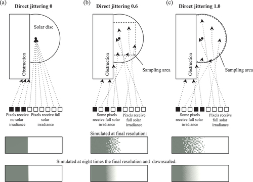The angular opening is often set at a constant of 0.533${ }^{\circ }$, which is an acceptable simplification since this angle fluctuates between 0.5399${ }^{\circ }$ (perihelion) and 0.5219${ }^{\circ }$ (aphelion), indicating a maximum difference of only four percent (Trujillo 2014). On the other hand, Radiance’s deterministic algorithm only uses a single ray to sample the sun, simplifying the sun to a point source neglecting its actual angular size (Fig. 2a).

Fig. 2. Radiance’s deterministic ray tracing algorithm without (a) and with direct jittering set to 0.6 (b) and 1.0 (c).

1.3. Existing methods to simulate solar penumbras and pinhole projections with Radiance

To simulate visually smooth penumbras and pinhole projections using Radiance’s simplified sun model and deterministic algorithm, (post) processing interventions are available. The general recommendation is to use the direct jittering algorithm (-dj) parameter, available in Radiance rpict (Ward 2023b), simulate the image at a higher resolution, and subsequently downscale the image during postprocessing (Ward et al. 2021). The direct jittering algorithm superimposes a square over a light source and randomly samples rays at specific positions within this square. The size of the square, relative to the light source’s dimensions, is controlled by setting direct jittering between 0.0 to 1.0. To simulate penumbras, a direct jittering value of 0.6 is typically recommended (Ward et al. 2021). Notably, since Radiance version 4.0, an exception is implemented for circular light sources such as the sun. In this case, when setting direct jittering to 1.0, rays are not sampled over a square but over a circle defined by a Philip Nowell map (Ward 2009). The direct jittering algorithm does not take into account the limited visibility of a light source due to any obstructions (Fig. 2b,c). Consequently, the shadow border will appear as a noisy pixel boundary, wherein some pixels receive the full solar irradiance while others receive none. Moreover, if the superimposed square is proportionally larger than the solar disc’s size (typically observed with direct jittering settings slightly below 1.0), rays may be aimed beside the solar disc, leading to no solar irradiance. The noisy pixel boundary can be transformed into a visually smooth penumbra by simulating an image at a higher resolution, and subsequently downscaling the image (Fig. 2). This technique is commonly known as supersampling anti-aliasing (Jiang et al. 2014).

Although, Radiance (post)processing interventions can generate solar penumbras and pinhole projections that appear visually accurate (Fig. 2), their accuracy and applicability are uncertain. In terms of accuracy, two notable limitations arise when simulating penumbras and pinhole projections using the direct jittering algorithm. First, simulated penumbras and pinhole projections rely on a random process rather than accurately determining the visible portion of the sun for a specific location. Second, the visually smooth penumbras are achieved by downscaling, a post-processing intervention that involves averaging luminances of multiple pixels into one. This process may not provide an accurate representation of reality. In terms of applicability, achieving smooth penumbras and pinhole projections with the direct jittering algorithm necessitates simulating images at an approximately eight times higher resolution, considerably impacting the simulation time and file size. A quick test shows that simulating at an eight times higher resolution takes approximately 64 times longer. This poses a challenge when using Radiance to simulate virtual reality (VR) environments, as done in recent studies (Chamilothori, Chinazzo, et al. 2019a; Fathy et al. 2023; Moscoso et al. 2021, 2022), since very high resolutions are required, even before considering simulating at an eightfold higher resolution. Therefore, more efficient methods for simulating solar penumbras and pinhole projections are needed.

1.4. Research aim

For daylight research and exacting daylighting design, accurate and efficient simulation of solar penumbras and pinhole projections holds importance. However, the accuracy and applicability of simulating these effects using existing Radiance methods are unclear. To address this, we present a validation of the existing Radiance approach (direct jittering and downscaling) and developed Radiance-based approaches that can accurately and efficiently simulate solar penumbras and pinhole projections.

2. Method

The applied method consists of three parts. First, three Radiance-based approaches to simulate solar penumbras and pinhole projections are presented. Second, we assess the validity of each of these approaches against real-world measurements. Third, we evaluate the applicability of the three approaches by examining simulation times and resulting file sizes using a reference case.

2.1. Three Radiance-based approaches to simulate solar penumbras and pinhole projections

To simulate solar penumbras and pinhole projections with Radiance, three approaches were considered: using direct jittering and downscaling, simulating the contribution of the sun through Radiance’s stochastic calculation, and subdividing the sun into many small suns. The approaches are discussed in the following sections and illustrated in Fig. 3. For each approach, the simulation parameters for Radiance rpict are given in Table 1.

Fig. 3. Three Radiance-based simulation approaches to generate solar penumbras and pinhole projections.

Table 1. Parameters used for simulations in Radiance rpict for each simulation approach.

Simulation approach	Deterministic algorithm parameters					Stochastic algorithm parameters
	-ps	-dj	-ds	-dt	-dc	-ab	-ar	-aa	-ad	-as	-lr	-lw
Direct jittering	1	0.6 & 1.0	0.1	0.05	0.5	2	64	0	256	0	7	0.001
Stochastic calculation	4	0	0.25	0.05	0.5	2	0	0	524,288	262,144	8	0.000003
Many suns	4	0	0.02	0	1	4	128	0.1	4096	2048	8	0.000003

2.1.1. Direct jittering and downscaling

Two values of direct jittering (-dj parameter) were investigated: 0.6 and 1.0. These direct jittering values were chosen since a value of 0.6 is typically recommended for simulating penumbras (Ward et al. 2021), while a value of 1.0 should theoretically provide accurate penumbras since rays are jittered over the complete angular size (disc) of the sun (Fig. 2c). Simulations were conducted at eight times the final resolution because after downscaling, no further reduction in image noise, particularly in penumbra smoothness, was observed when using higher resolutions. Simulation parameters were defined based on previous work (Stock 2003) and recommendations (Ward et al. 2021). Downscaling the resolution of the images was done using Radiance pfilt (Ward 2024) with a Gaussian filter set at a radius of 0.7 (Stock 2003). From here on, we refer to this method of simulating an image at an eightfold resolution with the direct jittering algorithm enabled, and subsequently downscaling the resulting image, as direct jittering, followed by the respective -dj parameter setting (i.e. 0.6 or 1.0).

2.1.2. Stochastic calculation

Radiance employs a stochastic (random) algorithm to simulate the contribution of reflected light or extended (i.e. large solid angle) light sources such as skylight. In this algorithm, at every sampling point in a scene, a large number of rays are sent out since light could arrive from any direction. Using this algorithm to stochastically sample the sun can theoretically provide more accurate penumbras (Ward et al. 2021) and pinhole projections, given that the complete angular size (of the solar disc) is sampled. However, this approach requires substantial computational resources, as approximately ${10}^5$ rays are needed for each pixel in a typical scene with both a sky and (visible) sun, to ensure that a single ray samples the sun (Mardaljevic 1995). The number of rays dispatched for each pixel is controlled by the number of ambient divisions (-ad parameter), which was hence set to a relatively high value of 524,288. Similarly, the number of ambient supersamples (-as parameter) determines the additional rays generated in areas with high variance, particularly the shadow border in this scenario. Therefore, this parameter was also set to a relatively high value of 262,144. Typically, irradiance caching is used to increase the speed of the stochastic calculation at the cost of introducing some minor error. Yet, for accurate simulation of direct sunlight using the stochastic algorithm, irradiance caching needs to be disabled by setting the ambient accuracy (-aa parameter) to zero. The number of ambient bounces (-ab parameter) was set to 2 to limit exceptional simulation times. The sun was stochastically sampled by defining it using Radiance’s glow material definition.

2.1.3. Many suns

A Radiance “standard” sun can be subdivided by filling its angular opening with many small openings, i.e. a lot of small sun descriptions. If the sun is subdivided in such a way, Radiance’s deterministic algorithm will only sample the visible suns, generating penumbras and pinhole projections. We developed a stencil method to transform a typical Radiance sun description to a description with a large number of small suns within the angular opening of a normal sun (de Vries 2024). In this method, an image of the sun is simulated with a camera position looking directly toward the sun. Depending on the dimensions of this image, the sun consists of a certain number of pixels. For every sun pixel, a direction vector is generated and used to create a new sun description with many small suns. A total of 632 small suns were used since through visual inspection of the outcomes across different subdivision ranges, no further improvement was observed when using more suns. Radiance’s selective source testing algorithm (controlled by the direct threshold, -dt parameter) and direct jittering were turned off to make sure that the contributions of all small suns were included.

2.2. Method: accuracy of the three simulation approaches

To validate the accuracy of solar penumbras and pinhole projections generated by the three simulation approaches (Fig. 3), the errors against real-world measurements were determined. In daylighting studies, an error of 20% is deemed typical for illuminance (sensor point) simulations (Jones and Reinhart 2015). Similarly, a study comparing mean illuminances in High Dynamic Range (HDR) images from real-world measurements and simulations using the Perez sky model also found errors within this range (Jones and Reinhart 2017). In this study, we maintain the same acceptable error threshold of 20%.

Building on existing methods for pixel-level comparisons of HDR images (Inanici 2005), we developed a novel method to investigate the accuracy of solar penumbras and pinhole projections in terms of dimensions. First, HDR images were captured under real-world conditions, depicting various semi-controlled solar penumbras and pinhole projections. Second, a simulation model was constructed of the same environment, with the same, although approximated, external (sky) conditions, and validated for predicting average luminances in the scene. Third, the three simulation approaches were employed to generate HDR images of the solar penumbras and pinhole projections, to allow pixel-level comparisons between the simulated and real-world measured HDR images. Lastly, the dimensions of the penumbras and pinhole projections in the measured and simulated HDR images were quantified and compared to determine the accuracy of the three simulation approaches. An overview of the applied method is shown in Fig. 4.

Fig. 4. Overview of the method to validate each of the three Radiance-based simulation approaches for generating solar penumbras and pinhole projections against real-world measurements.

2.2.1. Capturing real-world HDR images

To capture real-world solar penumbras and pinhole projections, an experimental setup consisting of an opaque plate with a small opening and a projection surface was created (Fig. 5). The plate was fitted onto a rail, allowing the distance between the plate and the projection surface to be changed, resulting in various penumbras and pinhole projections. Two plates measuring 120 by 120 mm were used, one with a circular opening of 2.31 mm in diameter, and the other with a square opening of 5 by 5 mm. The rail had a length of four meters and the projection surface, positioned perpendicular to the rail, was 840 by 600 mm and had a grid with 50 mm spacing. The opaque plates were slightly elevated above the rail, to allow placement of a luminance camera at the end of the rail, facing the projection surface.

Fig. 5. Measurement setup to capture various solar penumbras and pinhole projections.

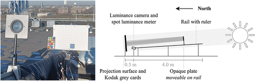
The setup was positioned on the roof of the Vertigo building at the Eindhoven University of Technology campus (Latitude: 51.44ºN, Longitude: 5.49ºE) at 58 meters from the ground to reduce interference by the surroundings. No structures of similar or greater height were within 200 meters south. Reflective objects on the roof were covered with black cloth. The setup faced true south and was slightly tilted at a fifteen degrees angle to approximate the solar altitude. The RGB reflectances of all materials of and near the setup were measured using a Konica Minolta Spectrophotometer CM-2600d (Table 2). A Digital Single-Lens Reflex (DSLR) camera (Canon EOS 60D with a Sigma 4.55 mm circular fisheye lens) was fixed at the northern end of the rail. This camera was set to take seven images (of 1202 by 1202 pixels) with differing exposures, which were combined to an HDR image, and will be referred to as a Luminance camera. Two gray Kodak cards were placed adjacent to the projection surface and a handheld spot luminance meter (Konica Minolta LS-150) was positioned at a slight angle relative to the projection surface. The plates were systematically moved over the rail, in increments of twenty centimeters, resulting in a total of eighteen positions. A total of thirty-six different solar penumbras and pinhole projections were captured using both plates. For each position, an HDR image was taken with the luminance camera, and the luminances of the two gray cards were measured using the handheld spot luminance meter. A weather station at the site measured the direct normal and diffuse horizontal irradiance every minute. All measurements were conducted on the 18th of January 2023 between 11:30 and 13:30 under clear sky conditions.

Table 2. Measured material properties (red, green, and blue reflectances) of objects of and near the experimental setup.

Surface	Red reflectance	Green reflectance	Blue reflectance
Projection surface	0.902	0.892	0.859
Projection surface grid	0.113	0.284	0.089
Metal plate	0.251	0.243	0.241
Wooden plate	0.449	0.261	0.154
Rail	0.043	0.043	0.044
Roof tile	0.069	0.055	0.045

The HDR images were processed by nullifying the exposure, cropping the borders, applying a fisheye and vignetting correction, and conducting a photometric adjustment based on the luminances measured on the Kodak gray cards, following the procedure described by Pierson et al. (2021). The average photometric adjustment was 0.86, with a standard deviation of 0.04. The sRGB values of the images were converted to luminances using equation 1 (Pierson et al. 2021).

(1) $\begin{array}{rl}& \mathit{L}=179\times \left(\mathit{R}\times 0.2126+\mathit{G}\times 0.7152\right.\\ & \left.+\mathit{B}\times 0.0722\right)\end{array}$(1)

2.2.2. Simulating HDR images

A dynamic model of the experimental setup was constructed in Rhino 7 with Grasshopper, allowing the plate to be modeled at multiple positions along the rail. Model attributes were based on the measured material properties (Table 2) and object dimensions (Fig. 5). A plane was modeled at 58 meters height to represent the roof. Moreover, a virtual camera, with the same lens type and position as the (real-world) luminance camera, was modeled. All materials were defined using Radiance’s plastic type, with the specularity and roughness parameters set to zero, assuming perfectly diffuse reflection. Radiance gendaylit (Delaunay et al. 2023) was used to create Perez-based sky descriptions from the weather station data.

2.2.2.1. Validation of the simulation model

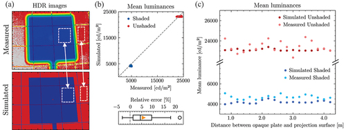
Before the simulation model can be used to investigate the accuracy of the three simulation approaches, the model must be validated in terms of predicting average luminances in HDR images, to make sure that no considerable modeling errors are present. Mean luminance values in the measured and simulated HDR images were compared for eighteen positions on the rail. Since two different opaque plates were used in the experiment, a total of thirty-six different simulations were conducted. The HDR images were simulated using Radiance rpict, without penumbras and pinhole projections, i.e. assuming a typical Radiance simulation. Simulation parameters as specified in Table 3 were used, based on recommended parameters for accurate simulations (Ward et al. 2021). The luminances of all pixels were extracted for a completely shaded (umbra) and unshaded area of the projection surface, as shown in Fig. 6a. For the measured HDR images, care was taken to avoid using areas exhibiting speckles with high luminance values, presumably stemming from specular reflections of sunlight on the projection surface. From each image, the mean luminance $L_a$ of the shaded and unshaded areas was computed. The resulting measurement and simulation points are clustered in Fig. 6b in two categorical groups. Next, the relative mean bias error ($\mathrm{MB}{\mathrm{E}}_{\mathrm{rel}}$) between the measured and simulated mean luminances of n images was computed:

Table 3. Radiance rpict parameters for validating the simulation model.

Deterministic algorithm parameters					Stochastic algorithm parameters							Resolution
-ps	-dj	-ds	-dt	-dc	-ab	-ar	-aa	-ad	-as	-lr	-lw	-x	-y
4	0	0.02	0	1	4	128	0.1	4096	2048	8	0.000003	4096	4096

Fig. 6. Validation of the simulation model for predicting mean luminances. (a) The used areas in the simulated and measured HDR images to compute the mean luminances. (b) Agreement between the thirty-six measured and simulated mean luminances. The line of equality is indicated by a dashed line. (c) The measured and simulated mean luminances for each position on the rail.

(2) $\begin{array}{rl}& \mathrm{MB}{\mathrm{E}}_{\mathrm{rel}}=100\mathrm{\%}\times \frac{1}{n}\\ & \sum _{\mathit{i}=1}^n\frac{{\mathit{L}}_{\mathit{a},\mathrm{measured},i}-L_{\mathit{a},\mathrm{simulated},i}}{L_{\mathit{a},\mathrm{measured},i}}\end{array}$(2)

Additionally, the relative root mean square error $\mathrm{RMS}{\mathrm{E}}_{\mathrm{rel}}$ was determined:

(3) $\mathrm{RMS}{\mathrm{E}}_{\mathrm{rel}}=100\mathrm{\%}\times \sqrt{\frac{1}{n}\sum _{\mathit{i}=1}^n{\left(\frac{{\mathit{L}}_{\mathit{a},\mathrm{measured},i}-L_{\mathit{a},\mathrm{simulated},i}}{L_{\mathit{a},\mathrm{measured},i}}\right)}^2}$(3)

Relative values are used because the unshaded areas had approximately five times higher mean luminance levels than the shaded areas but also to facilitate comparison between studies. The $\mathrm{MB}{\mathrm{E}}_{\mathrm{rel}}$ of the simulated luminances was 5.8%, the $\mathrm{RMS}{\mathrm{E}}_{\mathrm{rel}}$ 8.3%, and only eight out of thirty-six comparisons had an error larger than 10%. This error is well within the typical error margin of 20%, deeming the model adequate to investigate solar penumbras and pinhole projections.

The measured and simulated mean luminances for each position on the rail are shown in Fig. 6c. Each measurement, and corresponding simulation, was done under a certain sky condition and time of day. As a result, the presented luminances can be considered categorical variables, accounting for the observed slight fluctuations. In theory, moving the plate further away from the projection surface should result in a very small increase in luminance because the solid angle of the sky blocked by the plate is reduced. However, no significant trends were found in the presented luminances.

2.2.2.2. Simulating solar penumbras and pinhole projections

HDR images of the thirty-six different penumbras and pinhole projections were generated using the three simulation approaches and Radiance rpict. For the direct jittering approach, two values of direct jittering were used, resulting in a total of 144 unique HDR images. For each simulation approach, parameters as specified in Table 1 were used, and the image resolution was set to 4096 by 4096 pixels. All simulations were executed as single-core processes on a high-performance computing server (AMD EPYC 7452 (2.35 GHz) with 8 GB RAM/core) using bash scripts. The Radiance RGB values of the simulated HDR images were converted to luminances using equation 4 (Pierson et al. 2021).

(4) $\begin{array}{rl}& \mathit{L}=179\times (\mathit{R}\times 0.2651+\mathit{G}\times 0.6701\\ & +\mathit{B}\times 0.0648)\end{array}$(4)

2.2.3. Analysis of solar penumbras and pinhole projections

The accuracy of solar penumbras and pinhole projections generated by the three simulation approaches was investigated by visual and quantitative analyses. First, real-world and simulated HDR images of solar penumbras and pinhole projections were juxtaposed to facilitate visual comparisons of image noise and overall fidelity. Second, quantitative analyses were conducted to investigate the dimensions of the real-world and simulated penumbras and pinhole projections. All analyses were performed in Python 3.9.

2.2.3.1. Visual analyses

To compare the penumbras and the overall fidelity of the HDR images, all images were cropped to show only the region shaded by the opaque plate, converted into false-color representations, and juxtaposed. For visual comparisons of the pinhole projections’ dimensions, pixels corresponding to a 60 by 60 mm area on the projection surface, centered around the pinhole projection, were extracted from the HDR images. To be able to distinguish the pinhole projections, luminance normalization was employed since the projections only had small luminance differences compared to the background. This normalization consisted of applying a (linear) normalization factor to all pixel luminances to achieve an equal background luminance of the completely shaded parts (umbra).

2.2.3.2. Quantitative analysis of solar penumbra dimensions

To compute the length of a penumbra captured in an HDR image, luminance values were extracted along a line perpendicular to the shadow boundary (Fig. 7a). In the extracted luminance values, a relative dip is visible at the grid intersection points (for example at 40 pixels on the x-axis) since the reflectance of the grid is lower than the reflectance of the white projection surface (Table 2). The number of pixels per mm was computed by counting the number of pixels between the grid points, allowing conversion to a mm scale (Fig. 7b). Next, the penumbra length was extracted by identifying the length over which a substantial (consistent) change in luminance level is present. To minimize the impact of (real-world) measurement errors, i.e., fluctuations in the recorded luminance levels, curve fitting of a shadow function was applied (Fig. 7c). Shadow functions were developed in aerospace science to describe the solar penumbra cast by Earth into space but are deemed applicable to describe a solar penumbra on Earth. These functions represent the border of Earth’s shadow in space using a hyperbolic tangent (Escobal 1976; Hubaux et al. 2012). Based on these functions, we formulated an equation with luminance $\mathit{L}$ as the dependent variable and a hyperbolic tangent function with three unknown variables $\mathit{a}$, $\mathit{b}$, and $\mathit{c}$:

Fig. 7. Computing penumbra lengths from HDR images by extracting pixel luminances (a) and grid positions (b), fitting an equation (c), and taking the length corresponding to 90% of the luminance difference (d). The location of the line from which pixel luminances were extracted is indicated by a white line in panel (a).

(5) $\mathit{L}=\mathit{a}+\mathit{b}\times \mathit{tanh}(\mathit{c})$(5)

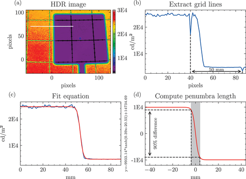
The unknown variables can be adjusted to curve fit the function to the (line) luminance data extracted from the HDR images. Curve fitting was performed using Python’s SciPy library (Virtanen et al. 2020).

From the curve-fitted function, the penumbra length cannot be simply determined by taking the difference between the absolute minimum and maximum because the hyperbolic tangent leads to flattening before reaching the extreme values. Instead, we defined the penumbra length as the length corresponding to 90% of the luminance difference between the minimum and the maximum of the curve-fitted equation (Fig. 7d). The penumbra lengths for the eighteen positions on the rail were extracted from the measured and simulated HDR images and plotted in one figure. For each simulation approach, the $\mathrm{MB}{\mathrm{E}}_{\mathrm{rel}}$ and $\mathrm{RMS}{\mathrm{E}}_{\mathrm{rel}}$ between the measured and simulated penumbra lengths of all distances between the plate and the projection surface were computed.

2.2.3.3. Quantitative analysis of solar pinhole projection dimensions

To quantify the pinhole projection diameters, the following steps were taken. The simulated and measured HDR images were cropped to only display the pinhole projections. Using Python’s OpenCV library (Bradski 2000), a Hough Circles transform, based on the Hough Gradient Method, was used to detect the boundaries of the pinhole projections. The Canny edge detection threshold was set to 80, and the accumulator threshold was set to 18. These values were found after trial and error to determine settings that consistently identified the pinhole projections. Identified pinhole projections were manually verified to correct any potential misidentifications due to the grid on the projection surface. If misidentification occurred, the respective image was excluded from the analysis. Utilizing the pixel-to-millimeter conversion (Fig. 7c), the pinhole projection diameter corresponding to each distance between the opaque plate and the projection surface was computed. For each simulation approach, the $\mathrm{MB}{\mathrm{E}}_{\mathrm{rel}}$ and $\mathrm{RMS}{\mathrm{E}}_{\mathrm{rel}}$ were calculated against the measured pinhole projection diameters.

2.3. Method: applicability of the three simulation approaches

The applicability of the three simulation approaches was evaluated through an analysis of simulation times and file sizes. A reference office model designed for comparative analyses of various façade and lighting solutions was used for this comparison (Reinhart et al. 2013). This office model includes a south-facing window and has a depth of more than three times the window head height. A virtual camera was positioned at the center of the office (-vp 2.0 5.0 1.8, -vh 80, and -vv 80), facing the window (-vd 0 –1 0 and -vu 0 0 1). The sun was positioned to cast sunlight in the room and the window blinds were removed from the model. Using the three simulation approaches, HDR images of 4096 by 4096 pixels (final resolution) were simulated using Radiance rpict, with parameters as specified in Table 1, using the same server as for the experimental images. For the direct jittering approach, only direct jittering 1.0 was used since no differences in simulation times and file sizes were expected when changing this parameter.

3. Results

The results section consists of two parts. First, we present the accuracy of the three simulation approaches for simulating solar penumbras and pinhole projections. Second, we present the applicability of these approaches in terms of simulation time and file size.

3.1. Results: accuracy of the three simulation approaches

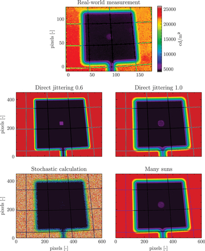
Thirty-six different solar penumbras and pinhole projections were measured and simulated, resulting in a total of 180 HDR images (36 measured and 144 simulated). A typical measurement, a plate with a circular opening at 1.6 m from the projection surface, and the corresponding simulations are shown in Fig. 8. No differences in image fidelity or noise were observed for the other distances between the opaque plate and the projection surface.

Fig. 8. Measured and simulated HDR images of an opaque plate with a circular opening at 1.6 m from the projection surface.

3.1.1. Measured and simulated solar penumbras

The penumbra lengths from measured and simulated HDR images, plotted against the distance between the opaque plate and the projection surface, are shown in Fig. 9. The $\mathrm{MB}{\mathrm{E}}_{\mathrm{rel}}$ and $\mathrm{RMS}{\mathrm{E}}_{\mathrm{rel}}$ of simulated penumbra lengths using each of the three approaches are given in Table 4. A positive $\mathrm{MB}{\mathrm{E}}_{\mathrm{rel}}$ indicates that the simulated penumbra length is overpredicted, while a negative error indicates underprediction compared to the real-world measurements. The $\mathrm{MB}{\mathrm{E}}_{\mathrm{rel}}$ of penumbras simulated using direct jittering 0.6 and 1.0 are 38.5% and −5.92%, indicating high underprediction and slight overprediction, respectively. Penumbras simulated using the stochastic calculation show a $\mathrm{MB}{\mathrm{E}}_{\mathrm{rel}}$ of −0.32%, suggesting, on average, a close match to the real-world measurements. However, for this approach, considerable fluctuations are present between measurements, as indicated by the $\mathrm{RMS}{\mathrm{E}}_{\mathrm{rel}}$ of 14.7%. These fluctuations may largely be attributed to image noise, as visible in Fig. 8. Penumbras simulated using many suns provided a close match to the real-world measurements, with only slight fluctuations ($\mathrm{MB}{\mathrm{E}}_{\mathrm{rel}}$: 0.72% and $\mathrm{RMS}{\mathrm{E}}_{\mathrm{rel}}$: 5.20%).

Fig. 9. Measured and simulated (using three simulation approaches) solar penumbra lengths across different distances between the opaque plate and the projection surface.

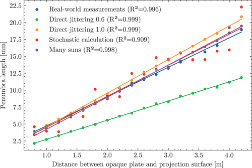
Table 4. Relative mean bias errors ($\mathrm{MB}{\mathrm{E}}_{\mathrm{rel}}$) and relative root mean square errors ($\mathrm{RMS}{\mathrm{E}}_{\mathrm{rel}}$) of penumbra length and pinhole projection diameter comparing simulations using three Radiance-based approaches against real-world measurements.

Simulation approach	Penumbra length		Pinhole projection diameter
	$\mathrm{MB}{\mathrm{E}}_{\mathrm{rel}}$	$\mathrm{RMS}{\mathrm{E}}_{\mathrm{rel}}$	$\mathrm{MB}{\mathrm{E}}_{\mathrm{rel}}$	$\mathrm{RMS}{\mathrm{E}}_{\mathrm{rel}}$
Direct jittering 0.6	38.5%	38.6%	–	–
Direct jittering 1.0	−5.92%	7.55%	−11.7%	13.9%
Stochastic calculation	−0.32%	14.7%	–	–
Many suns	0.72%	5.20%	−2.30%	8.45%

3.1.2. Measured and simulated solar pinhole projections

Measured and simulated solar pinhole projections, resulting from opaque plates with a circular or square pinhole, are given in Figs. 10 and 11. The top row indicates the real-world measurements, while the subsequent rows show the simulations using the three approaches. Both figures use the same restricted luminance range to distinguish the pinhole projections, but this leads to most pixels in the pinhole projections being saturated. Notably, in both figures, it is evident that simulations using direct jittering 0.6 produce square-shaped pinhole projections, aligning with expectations based on the sampling area (Fig. 2). Simulations using the stochastic calculation resulted in dispersed speckles of light within the circular area where the pinhole projections should be but did not create a coherent visible pinhole projection for either circular or square pinholes.

Fig. 10. Grey shaded images of real-world and simulated, using three approaches, solar pinhole projections. The pinhole projections result from an opaque plate with a circular pinhole (diameter 2.31 mm) at various distances from the projection surface.

Fig. 11. Grey shaded images of real-world and simulated, using three approaches, solar pinhole projections. The pinhole projections result from an opaque plate with a square pinhole (5 by 5 mm) at various distances from the projection surface.

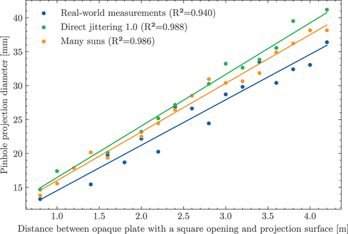
The diameters of measured and simulated pinhole projections resulting from an opaque plate with a square opening (5 by 5 mm) are shown in Fig. 12, and the corresponding $\mathrm{MB}{\mathrm{E}}_{\mathrm{rel}}$ and $\mathrm{RMS}{\mathrm{E}}_{\mathrm{rel}}$ are shown in Table 4. Only simulations using direct jittering 1.0 or many suns were included since using direct jittering 0.6 or the stochastic calculation did not provide clear circular pinhole projections, which are needed for the Hough Circles algorithm. Moreover, two out of eighteen measured and six out of thirty-six simulated pinhole projections were excluded from this analysis as the algorithm was unable to identify or misidentified the pinhole projection. Similar to the findings regarding penumbra lengths, simulations using direct jittering 1.0 tended to overpredict the pinhole projection diameters, with a $\mathrm{MB}{\mathrm{E}}_{\mathrm{rel}}$ of −11.7%. Using the many suns approach, the pinhole projection diameters closely matched the real-world measurements, although slightly underpredicting them, with a $\mathrm{MB}{\mathrm{E}}_{\mathrm{rel}}$ and $\mathrm{RMS}{\mathrm{E}}_{\mathrm{rel}}$ of −2.30 and 8.45%. The other opaque plate had a smaller opening (2.31 mm diameter), resulting in only slight luminance differences between the pinhole projections and the background. Combined with fluctuations in the background luminance, it was not possible to extract the pinhole projection diameters from the real-world measurements using this plate, and thus these are not included in the analysis.

Fig. 12. Measured and simulated (using two simulation approaches) solar pinhole projection diameters shown across different distances between the opaque plate with a square opening and the projection surface.

3.2. Results: applicability of the three simulation approaches

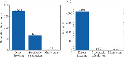
Using the reference office model (Reinhart et al. 2013), simulation times (Fig. 13a) and file sizes (Fig. 13b) of the three simulation approaches were computed. For these comparisons, HDR images of 4096 by 4096 pixels were simulated with parameters as specified in Table 1, as well as only one direct jittering value (1.0). Simulating an HDR image using many suns took 3.1 hours, which is approximately 21 times faster compared to using the stochastic calculation, and even 56 times faster than using direct jittering. The many suns approach offers a timeframe measured in hours, a stark contrast to the days required by the other two approaches. Images generated with the many suns or stochastic calculation approaches are similar in size, while the direct jittering approach requires the image to be generated at eight times the final resolution, creating a large (4194 MB) high-resolution file. After downscaling, the image simulated with direct jittering becomes comparable in size to the other approaches.

Fig. 13. Simulation times (a) and file sizes (b) for reference case simulations using the three Radiance-based approaches.

4. Discussion

In Radiance simulations, solar penumbras and pinhole projections, two effects of sunlight, are often not included due to a simplified sun model and deterministic algorithm. This study investigated the accuracy and applicability of different Radiance-based simulation approaches for generating these effects of sunlight. Three simulation approaches were applied: using direct jittering and downscaling, simulating the contribution of the sun through the stochastic calculation, and simulating many small suns. Accuracy was evaluated by calculating the errors of simulated solar penumbra lengths and pinhole projection diameters against real-world measurements. Applicability was assessed through simulations using a reference office model, recording simulation time and resulting file size. First, we discuss the accuracy and applicability of the simulation approaches, followed by the limitations of this study, and lastly the recommendations and outlook.

4.1. Discussion: accuracy of the three simulation approaches

In terms of accuracy, simulations using many suns or direct jittering 1.0 provided the best results. The many suns approach resulted in the lowest $\mathrm{RMS}{\mathrm{E}}_{\mathrm{rel}}$, at 5.20% for simulating penumbra lengths, and 8.45% for simulating pinhole projection diameters. In a similar range, the direct jittering 1.0 approach resulted in a $\mathrm{RMS}{\mathrm{E}}_{\mathrm{rel}}$, of 7.55% and 11.47% for simulating penumbra lengths and pinhole projection diameters, respectively. However, simulations with direct jittering 1.0 showed a consistent overprediction of the penumbra lengths ($\mathrm{MB}{\mathrm{E}}_{\mathrm{rel}}$: −5.92%) and pinhole projection diameters ($\mathrm{MB}{\mathrm{E}}_{\mathrm{rel}}$: −11.7%), while simulations with many suns did not consistently under or overpredict both effects. These overpredictions in simulations with direct jittering 1.0 likely stem from the eightfold downscaling of the image during postprocessing, needed to create a noise-free penumbra boundary (Fig. 2). In this process, multiple pixels are combined, resulting in smoother luminance transitions and hence a slight increase in penumbra length. It should be noted that in terms of image fidelity, some noise persisted in the pinhole projections even after eightfold downscaling (see Figs. 10 and 11). However, these outcomes show that using both the many suns or direct jittering 1.0 approaches, solar penumbras and pinhole projections can be simulated with a typical error well below 20%.

Using the stochastic calculation or direct jittering 0.6 approaches did not provide accurate results and did not allow quantification of the pinhole projection diameters due to a lack of coherent (circular) projections. Direct jittering 0.6, the generally recommended value (Ward et al. 2021), led to substantial underprediction of penumbra lengths ($\mathrm{MB}{\mathrm{E}}_{\mathrm{rel}}$: 38.54) and pinhole projection dimensions, as can be visually identified in Figs. 10 and 11. These results were anticipated, as rays were sampled over only a fraction of the sun’s area in this approach (Fig. 2). The square shape of the sampling area did not visibly affect the resulting penumbras but was evident in the pinhole projections. Using the stochastic calculation, with the tested parameters (Table 1), produced images with considerable noise, rendering this approach unsuitable for generating images of solar penumbras or pinhole projections with acceptable fidelity. Nonetheless, the mean penumbra lengths generated by simulations using the stochastic calculation have a very low $\mathrm{MB}{\mathrm{E}}_{\mathrm{rel}}$ at −0.32%, indicating that the entire sun’s size was sampled. However, the image noise caused substantial fluctuations ($\mathrm{RMS}{\mathrm{E}}_{\mathrm{rel}}$: 14.7%) in penumbra lengths of individual measurements (as visible in Fig. 9), dependent on which pixels were used to extract the luminance values (Fig. 7a). Only speckles of light were observed in the area where the pinhole projection should appear (see Figs. 10 and 11). This suggests that the number of randomly sampled rays at each pixel was insufficient to consistently reach the sun through the pinhole. Enhancing simulation parameters, particularly the -ad and -as parameters, has the potential to generate images with reduced noise and more coherent pinhole projections. However, it is worth noting that the images generated in this study with the stochastic calculation, based on a simple scene with minimal geometry, required approximately twelve days to simulate. Further increases in simulation parameters are likely to lead to considerably longer simulation times, particularly for scenes with more complex geometry, making this option impractical.

To summarize, these findings demonstrate that employing either the many suns or direct jittering 1.0 approaches allow accurate simulations of solar penumbras and pinhole projections, maintaining an error well below 20%. While the accuracy of penumbras simulated through the stochastic calculation was within this error range, this approach could not provide sufficiently noise-free images to be used for visualizations. The direct jittering 0.6 approach considerably underestimated penumbra lengths and, along with the stochastic calculation approach, did not provide coherent pinhole projections.

4.2. Discussion: applicability of the three simulation approaches

The applicability, i.e. simulation times and files sizes, of the aforementioned simulation approaches was compared by conducting simulations using a reference office model, with simulation parameters as specified in Table 1.

Generally, approaches that are based on tracing a large number of rays often lead to extensive simulation times, making them less favorable due to their reliance on substantial computational resources. Simulating an HDR image (4096 by 4096 pixels) of the reference model using many suns took 3.1 hours – a substantial improvement, being 21 and 56 times faster compared to using the stochastic calculation and direct jittering, respectively. However, this prompts the question, what is considered an acceptable simulation timeframe? Typically, durations extending to hours are deemed reasonable for most simulation purposes, while durations extending across multiple days become considerably less practical. Directly comparing simulation times reported by previous studies is challenging, as they are greatly influenced by model complexity, simulation parameters, and the type of computing system used. As an example, we consider previous studies that used Radiance to generate VR environments, simulating images at similar resolutions to the current study. These simulations did not have solar penumbras and pinhole projections, since all considered studies turned direct jittering off and did not apply any of the (other) discussed approaches. Simulating images for a study investigating various spaces with differing geometric complexities took between 12 to 48 hours per image (Rockcastle et al. 2017). For a simpler scene, albeit at a slightly lower resolution, the average simulation time was around 2.7 hours per image (Chamilothori et al. 2019a, 2019b). In this context, the 3.1 hours needed for simulating a typical scene using the many suns approach is deemed reasonable.

If needed, the simulation speed of the many suns approach can be improved by independently running Radiance’s deterministic and stochastic algorithms. The deterministic algorithm generates direct sunlight in a scene, including solar penumbras and pinhole projections, and thus relies on the many suns. Given that the many suns provide approximately the same irradiance in the scene as a normal (single) sun, the stochastic algorithm, responsible for computing reflected light contributions, can effectively run on just one (normal) sun, simplifying the calculation. In addition, a further speed improvement can be achieved by lowering the resolution of the simulation parameters or the number of suns, but requires careful evaluation of the impact on the resulting penumbras and pinhole projections.

Regarding the file size of the resulting simulated image, the need for (temporary) storage space is limited when using the many suns or the stochastic calculation approaches, as images can be simulated at the final resolution, or at two to four times the resolution for anti-aliasing purposes (Jiang et al. 2014). In the reference simulation case of this study, images produced using these approaches typically range between 12 and 16 MB. In contrast, direct jittering necessitates simulating images at an eightfold resolution, requiring 64 times more pixels and thus leading to considerably larger file sizes. In the reference case, this amounted to a file size of 4194 MB, requiring approximately 260 times more storage space compared to the other two approaches. Despite modern computing systems generally handling these file sizes well, issues might arise during file transfers between systems. Yet, the eightfold downscaling of images simulated with direct jittering considerably reduces the file sizes, making them comparable to those simulated with the other two approaches. This process can typically be performed on the same computing system where the initial images were simulated, effectively mitigating this potential issue.

It is also worth considering the ease of use of every simulation approach. Direct jittering is the most straightforward approach, as no modifications to a typical Radiance sun description are required. To use the stochastic calculation approach, the required modification is still fairly simple, i.e. only a single line needs to be changed in the Radiance sun description. This approach can also be implemented using Radiance rcontrib Ward (2023a), which automatically disables the ambient cache. However, it requires a more complex simulation setup, i.e. a definition of the view rays to create the image and a list of the sun and sky modifiers, unlike our approach based on rpict. Although generating many suns demands more extensive modifications to a Radiance sun description, it can be automated using a Python script available on GitHub (de Vries 2024), offering a viable option for implementation.

In short, the many suns approach stands out as the most practical in terms of simulation speed, providing an acceptable timeframe of hours. In contrast, both the direct jittering and the stochastic calculation approaches take considerably longer to simulate, extending to days. The resulting image file sizes of all approaches are, at least after post-processing, sufficiently small to be readily managed by modern computing systems. While the many suns approach is slightly more complex to implement than the stochastic calculation and direct jittering approaches, automation options are available.

4.3. Limitations of the study

Lighting simulation validations that combine real-world measurements and simulation models inherently introduce some uncertainties from measurement imprecision and modeling simplifications. Real-world measurement inaccuracies can result from measurement errors of the equipment (Pierson et al. 2021), changing sky conditions, and unforeseen reflections (Jones and Reinhart 2017). The simulation model used in the present study simplifies the geometry and the surroundings, as well as the sky luminance distribution by using a Perez sky model, introducing simulation errors (Ochoa et al. 2012). Although the simulation model validation revealed a $\mathrm{RMS}{\mathrm{E}}_{\mathrm{rel}}$ of only 8.3% for predicting average luminances of the shaded and unshaded projection surface, it is assumed that this error has some impact on the reported errors for the simulation approaches for generating solar penumbras and pinhole projections.

The image resolution (1202 by 1202 pixels) of the luminance camera used in the present study was limited, especially when considering the size of the pinhole projections in the images. For measurements using the opaque plate with a small circular opening, the limited number of pixels making up the pinhole projection (typically just 100), coupled with a low luminance difference and background noise (as evident in the real-world measurements in Fig. 10), made it impossible to extract the pinhole diameters using the Hough Circles algorithm. Moreover, for measurements using the plate with the larger square opening, the smallest pinhole projections typically consisted of just 200 pixels, which might have introduced some error. This may explain to some extent the larger $\mathrm{RMS}{\mathrm{E}}_{\mathrm{rel}}$ for the pinhole projection diameters compared to the penumbra lengths (Table 4). Still, the juxtaposed pinhole projections of real-world and simulated images in Figs. 10 and 11 show that they appear quite similar.

For any Radiance simulation, the chosen parameters will have a profound impact on the accuracy of the resulting image and the applicability of the simulation approach. In this study, parameters were derived from available literature and through guided experimentation. The selected parameters were chosen on the assumption that further increases, meaning a more complex and prolonged calculation, would not substantially impact image accuracy. In retrospect, the accuracy of the stochastic calculation approach is expected to improve by enhancing the parameter settings. Presently, images generated through this approach have considerable image noise, resulting in fluctuations in the extracted luminances. Increasing the parameters is anticipated to reduce image noise and subsequently enhance accuracy. Nevertheless, this would considerably prolong simulation times, making it impractical for routine use cases. Regarding applicability, simulation times could be expedited with lower resolution parameters, albeit potentially compromising accuracy. Nonetheless, we expect that even with lower parameters, the many suns approach will consistently offer the highest accuracy coupled with the highest simulation speeds, relative to the other approaches.

4.4. Recommendations and outlook

For daylighting research and design scenarios where accurate solar penumbras and pinhole projections are important, we recommend conducting Radiance simulations using the many suns approach. Especially for VR studies investigating the perception of natural lighting conditions, where high-resolution simulated images are needed, the many suns approach allows for more accurate solar penumbras and pinhole projections as well as a considerable increase in simulation speed compared to the direct jittering approach. However, for scenarios where only low-resolution images are required, the direct jittering approach can be considered since it is readily integrated in Radiance, albeit producing images with a slightly lower accuracy and in a longer simulation time.

The primary focus of this study was to investigate the accuracy of simulation approaches for generating images depicting solar penumbras and pinhole projections. Another envisaged application for these simulation approaches involves assessing the shading potential of enclosures composed of repetitive small architectural elements, e.g. meshes. In such assessments, the many suns approach is likely to provide more accurate luminances at a high spatial resolution, compared to using the direct jittering approach or simply not simulating penumbras. For visual comfort metrics that are sensitive to small areas of high luminance, such as the daylight glare probability (DGP) Wienold et al. (2019), this may have a significant impact. In practice, complex (repetitive) architectural elements are often modeled using bidirectional scattering distribution functions (BSDFs). With recent advances in the adequacy of (measurement-based) BSDFs for processing direct sunlight Ward et al. (2021); Wang et al. (2022), combining BSDFs with the many suns approach may be a viable option for glare evaluations that require a high spatial resolution. For these scenarios involving complex architectural elements, it may be necessary to assess the accuracy of Radiance’s ambient calculation, given that the present study focused on accurately simulating effects of direct sunlight.

Currently, integrating the many suns approach into Radiance requires a custom-made sun description. The underlying principle of the many suns approach involves subdividing the sun into smaller suns that are sampled individually. Introducing an option to subdivide a sun within Radiance would streamline the utilization of the many suns method in typical Radiance simulations. Furthermore, implementing this feature exclusively for the deterministic algorithm could achieve the aforementioned further speed improvement without needing to run separate simulations for Radiance’s deterministic and stochastic algorithms.

5. Conclusion

To facilitate daylight research and design that takes into account solar penumbras and pinhole projections, improved lighting simulation methods are needed that can accurately reproduce these effects. This study investigated the accuracy and applicability of simulating these effects using three Radiance-based methods. As a novelty, the accuracy was evaluated by calculating the errors of various simulated solar penumbra lengths and pinhole projection diameters against real-world measurements. The applicability, in terms of simulation speed and file size, was assessed through simulations using a reference office model. The method with the highest accuracy was subdividing a Radiance sun description into 632 small suns, with a root mean square error of 5.20% for penumbra lengths, and 8.45% for pinhole projection diameters. Using direct jittering over the full solar disc and an eightfold reduction of the image resolution provided only slightly larger errors (7.55% and 13.9%) but required 172.5 hours to simulate a typical scene, approximately a 56 times increase compared to the 3.1 hours needed for the subdivided sun. Lastly, relying solely on Radiance’s stochastic algorithm required 65.1 hours to simulate but could not provide visually noise-free images. Overall, the findings of this study show that subdividing a Radiance sun into many small suns is a practical and accurate method to incorporate solar penumbras and pinhole projections in Radiance simulations.

Acknowledgments

The authors would like to thank Prof. John Mardaljevic for his contributions in developing the Radiance simulation approaches and feedback on this manuscript and Dr. Adrie de Vries and Signify for their feedback and support on the project.

Disclosure statement

No potential conflict of interest was reported by the author(s).

Additional information

Funding

Sietse de Vries received funding from Intellight+, an Eindhoven Engine project.

References

- Abboushi B, Elzeyadi I, Taylor R, Sereno M. 2019. Fractals in architecture: the visual interest, preference, and mood response to projected fractal light patterns in interior spaces. J Environ Psychol. 61:57–70. doi: 10.1016/j.jenvp.2018.12.005.
- Baker NV, Fanchiotti A, Steemers K. 1993. Daylighting in architecture: a European reference book. 1st ed. Londen (UK): Routledge. p. 8.2.
- Bradski G. 2000. The opencv library. Dr Dobb’s J Software Tools. 25:120–125.
- Buie D, Monger AG, Dey CJ. 2003. Sunshape distributions for terrestrial solar simulations. Sol Energy. 74(2):113–122. doi:10.1016/S0038-092X(03)00125-7.
- Chamilothori K, Chinazzo G, Rodrigues J, Dan-Glauser ES, Wienold J, Andersen M. 2019a. Subjective and physiological responses to fac¸ade and sunlight pattern geometry in virtual reality. Build Environ. 150:144–155. doi: 10.1016/j.buildenv.2019.01.009.
- Chamilothori K, Wienold J, Andersen M. 2019b. Adequacy of immersive virtual reality for the perception of daylit spaces: comparison of real and virtual environments. LEUKOS. 15(2–3):203–226. doi: 10.1080/15502724.2017.1404918.
- Chamilothori K, Wienold J, Moscoso C, Matusiak B, Andersen M. 2022. Subjective and physiological responses towards daylit spaces with contemporary façade patterns in virtual reality: influence of sky type, space function, and latitude. J Environ Psychol. 82:101839. doi: 10.1016/j.jenvp.2022.101839.
- de Vries SW. 2024. Radynvr-genmanysuns: V1.0. doi: 10.5281/zenodo.11394339.
- Dee HM, Santos PE. 2011. The perception and content of cast shadows: an interdisciplinary review. Spat Cogn Comput. 11(3):226–253. doi:10.1080/13875868.2011.565396.
- Delaunay J, Wienold J, Sprenger W. 2023. Gendaylit. https://floyd.lbl.gov/radiance/man_html/gendaylit.1.html.
- Escobal PR. 1976. Methods of orbit determination. 2nd ed. Malabar (FL): Krieger Publishing Company.
- Fathy F, Mansour Y, Sabry H, Refat M, Wagdy A. 2023. Virtual reality and machine learning for predicting visual attention in a daylit exhibition space: a proof of concept. Ain Shams Eng J. 14(6):102098. doi: 10.1016/j.asej.2022.102098.
- Galasiu AD, Atif MR. 2002. Applicability of daylighting computer modeling in real case studies: comparison between measured and simulated daylight availability and lighting consumption. Build Environ. 37(4):363–377. doi: 10.1016/S0360-1323(01)00042-7.
- Hammond JH. 1981. The camera obscura, a chronicle. 1st ed. Bristol (UK): Adam Hilger Ltd.
- Hill AJ, Triantafyllidis G. 2023. Evaluation of emotions induced by biophilic lighting patterns using eeg and qualitative methods. In: Proceedings of the 30th Session of the CIE. Vol. 1. Ljubljana (Slovenia): CIE.
- Hubaux C, Lemaître A, Delsate N, Carletti T. 2012. Symplectic integration of space debris motion considering several earth’s shadowing models. Adv Space Res. 49(10):1472–1486. doi: 10.1016/j.asr.2012.02.009.
- Inanici M. 2005. Per-pixel lighting data analysis. Report No: lBNL-58659. Berkley: Ernest Orlando Lawrence Berkley National Laboratory. doi: 10.2172/891345.
- Jiang X, Sheng B, Lin WY, Lu W, Ma LZ. 2014. Image anti-aliasing techniques for internet visual media processing: a review. J Zhejiang Univ Sci C. 15(9):717–728. doi: 10.1631/jzus.C1400100.
- Jones NL, Reinhart CF. 2015. Validation of gpu lighting simulation in naturally and artificially lit spaces. In: Mathur J, and Garg V, editors. Proceedings of Building Simulation 2015: 14th Conference of IBPSA; Hyderabat (India): IBPSA. p. 1229–1236. doi: 10.26868/25222708.2015.2461.
- Jones NL, Reinhart CF. 2017. Experimental validation of ray tracing as a means of image-based visual discomfort prediction. Build Environ. 113:131–150. doi: 10.1016/j.buildenv.2016.08.023.
- Karaman-Madan Ö, Linders IK, Chamilothori K, de Kort YAW. 2023. Effects of dynamic light patterns with natural and non-natural temporal composition on reported stress recovery, fascination, and association with nature. In: The 30th Quadrennial Session of the CIE (CIE 2023); Ljubljana, Slovenia.
- Mardaljevic J. 1995. Validation of a lighting simulation program under real sky conditions. Lighting Res Technol. 27(4):181–188. doi: 10.1177/14771535950270040701.
- Mardaljevic J. 2001. The bre-idmp dataset: a new benchmark for the validation of illuminance prediction techniques. Lighting Res Technol. 33(2):117–134. doi: 10.1177/136578280103300209.
- Minnaert MGJ, Seymour L. 1993. Light and color in the outdoors. New York (USA): Springer New York. p. 417.
- Moscoso C, Chamilothori K, Wienold J, Andersen M, Matusiak B. 2021. Window size effects on subjective impressions of daylit spaces: indoor studies at high latitudes using virtual reality. LEUKOS. 17(3):242–264. doi: 10.1080/15502724.2020.1726183.
- Moscoso C, Chamilothori K, Wienold J, Andersen M, Matusiak B. 2022. Regional differences in the perception of daylit scenes across Europe using virtual reality. part i: effects of window size. LEUKOS. 18(3):294–315. doi: 10.1080/15502724.2020.1854779.
- Ng EY, Poh LK, Wei W, Nagakura T. 2001. Advanced lighting simulation in architectural design in the tropics. Autom Constr. 10(3):365–379. doi: 10.1016/S0926-5805(00)00053-4.
- Ochoa CE, Aries MBC, Hensen JLM. 2012. State of the art in lighting simulation for building science: a literature review. J Build Perform Simul. 5(4):209–233. doi: 10.1080/19401493.2011.558211.
- Perez R, Seals R, Michalsky J. 1993. All-weather model for sky luminance distribution—preliminary configuration and validation. Sol Energy. 50(3):235–245. doi: 10.1016/0038-092X(93)90017-I.
- Pierson C, Cauwerts C, Bodart M, Wienold J. 2021. Tutorial: luminance maps for daylighting studies from high dynamic range photography. LEUKOS. 17(2):140–169. doi: 10.1080/15502724.2019.1684319.
- Reinhart C, Breton P. 2009. Experimental validation of Autodesk® 3ds max® design 2009 and daysim 3.0. LEUKOS. 6(1):7–35. doi: 10.1582/LEUKOS.2009.06.01001.
- Reinhart CF, Andersen M. 2006. Development and validation of a radiance model for a translucent panel. Energ Buildings. 38(7):890–904. Special Issue on Daylighting Buildings. doi: 10.1016/j.enbuild.2006.03.006.
- Reinhart CF, Jakubiec JA, Ibarra D. 2013. Definition of a reference office for standardized evaluations of dynamic façade and lighting technologies. In: Proceedings of Building Simulation 2013: 13th Conference of IBPSA; Chambéry, France. p. 3645–3652. doi: 10.26868/25222708.2013.1029.
- Reinhart CF, Walkenhorst O. 2001. Validation of dynamic radiance-based daylight simulations for a test office with external blinds. Energ Buildings. 33(7):683–697. doi: 10.1016/S0378-7788(01)00058-5.
- Rockcastle S, Amundadottir ML, Andersen M. 2017. Contrast measures for predicting perceptual effects of daylight in architectural renderings. Lighting Res Technol. 49(7):882–903. doi: 10.1177/1477153516644292.
- Sigura V, Hansen EK, Clausen H. 2022. Designing natural atmosphere in office environment through daylight responsive dynamic lighting. In: IOP Conference Series: earth and Environmental Science. Vol. 1099. Copenhangen (Denmark): Institute of Physics. doi: 10.1088/1755-1315/1099/1/012029.
- Stock MJ. 2003. Radiance ambient and penumbra test v2.0. http://markjstock.org/radmisc/aa0_ps1_test/final.html.
- Trujillo JHS. 2014. Calculation of the shadow-penumbra relation and its application on efficient architectural design. Sol Energy. 110:139–150. doi:10.1016/j.solener.2014.08.043.
- Virtanen P, Gommers R, Oliphant TE, Haberland M, Reddy T, Cournapeau D, Burovski E, Peterson P, Weckesser W, Bright J, et al. 2020. Scipy 1.0: fundamental algorithms for scientific computing in python. Nat Methods. 17(3):261–272.doi:10.1038/s41592-019-0686-2.
- Wang T, Lee ES, Ward G, Yu T. 2022. Field validation of data-driven bsdf and peak extraction models for light-scattering fabric shades. Energy Build. 262:112002. doi: 10.1016/j.enbuild.2022.112002.
- Ward G. 1994. The radiance lighting simulation and rendering system. In: 21st Annual Conference on Computer Graphics and Interactive Techniques; NY (USA). p. 459–472.
- Ward G. 2009; Radiance 4.0 improvements.
- Ward G. 2023a. Rcontrib. https://floyd.lbl.gov/radiance/man_html/rcontrib.1.html.
- Ward G. 2023b. Rpict. https://floyd.lbl.gov/radiance/man_html/rpict.1.html.
- Ward G. 2024. Pfilt. https://radsite.lbl.gov/radiance/man_html/pfilt.1.html.
- Ward G, Shakespeare R, Ehrlich C, Mardaljevic J, Philips E, Apian-Bennewitz P. 2021. Rendering with radiance the art and science of lighting visualization. Vol. 1. Tacoma (WA): Randolph M. Fritz.g
- Ward G, Wang T, Geisler-Moroder D, Lee ES, Grobe LO, Wienold J, Jonsson JC. 2021. Modeling specular transmission of complex fenestration systems with data-driven bsdfs. Build Environ. 196:107774. doi: 10.1016/j.buildenv.2021.107774.
- Wienold J, Iwata T, Sarey Khanie M, Erell E, Kaftan E, Rodriguez RG, Yamin Garreton JA, Tzempelikos T, Konstantzos I, Christoffersen J, et al. 2019. Cross-validation and robustness of daylight glare metrics. Lighting Res Technol. 51(7):983–1013. doi: 10.1177/1477153519826003.