Including Dynamic Viewing Behavior in Determining Vertical Eye-Level Light: Does it Matter for Office Design?

ABSTRACT

When considering non-image-forming (NIF) light effects on people, knowing the light vertically at eye-level is necessary. However, people are dynamic in their behavior and constantly change their posture and viewing direction. This means that light measured vertically toward a constant direction might differ from the actual light that reaches people’s eyes. If the difference is large, occupant behavior might need to be included in lighting design measurements and simulations predicting the potential of NIF light effects. This paper presents an experiment on the difference between the actual dynamic eye-level light of office workers while seated at a desk (dynamic condition) and light measured statically toward a computer screen (static condition). Eye-level light conditions in relation to NIF effects were quantified using the melanopic Equivalent Daylight Illuminance (mEDI) and the relative alerting response (r_D). Measured dynamic mEDI was 4% to 10% larger than the static one. Analysis of r_D was not possible due to saturation of the response. The dominant face orientation was toward the computer screen, with a deviation in the horizontal and vertical direction within 15 degrees from the center. The results show that measuring and simulating personal light conditions of office workers statically toward a computer screen might be a small underestimation of actual eye-level light, but the relevance of this underestimation in lighting design practice is not evident.

KEYWORDS:

• Head rotation
• indoor lighting
• lighting simulation
• non-visual
• ocular light

1. Introduction

Light affects humans through the non-image-forming (NIF) system in multiple ways. The NIF responses include the regulation of the circadian system, the suppression of melatonin production, and acute alertness (Vetter et al. 2021). These responses have different spectral, spatial and temporal sensitivity to light than the known visual responses (Houser et al. 2021; Khademagha et al. 2016).

Since it is the eye that mediates the response of humans to light, lighting conditions at eye-level are important when considering the NIF effects of light. This means that measuring light on a horizontal plane – as is still common in lighting design standards focusing on visual performance – is not sufficient, but it needs to be supplemented by vertically measured light at eye-level (Altenberg Vaz and Inanici 2020; Knoop et al. 2019; Konis 2019; Spitschan et al. 2019).

Design recommendations for vertically measured light quantities have started to be developed (Brown et al. 2022) and it is possible that future lighting design standards will incorporate them. For such recommendations to be applied in practice, assumptions about the light falling onto a person’s eyes are needed. For offices, a common method to determine this amount of light is to measure it with or simulate it for a sensor in the vertical plane directed toward a computer screen (Abboushi and Safranek 2022; Brennan and Collins 2018; Potocnik and Kosir 2020; Zeng et al. 2021). In reality, people are dynamic in their natural behavior, change their posture and shift their viewing direction. Therefore the light exposure predicted by a static view assumption might differ significantly from the actual individual’s dynamic light exposure.

There are a handful of studies that investigated the difference between light measured vertically in a static direction and light measured following the dynamic behavior of an office occupant. van Duijnhoven et al. (2019) found that considering the changing view direction of office workers would result in approximately 5% increase in luminous exposure compared to a static direction toward the screen. In their study, the light distribution was not measured directly in the office environment that the participants worked in, but in a mock-up office. An important limitation is that their findings are based on observations of only six participants, making it difficult to draw strong conclusions. Sarey Khanie et al. (2017) found a significant difference between vertical illuminance measured statically toward a computer and gaze-driven (dynamic) vertical illuminance. They found that the dynamic illuminance was larger than the static one for tasks that required more thinking, but smaller for tasks that required reading from a computer. Specifically, for thinking tasks and vertical illuminance ranges that are less likely to cause glare (less than 3500 lx), they found that the mean dynamic illuminance was almost double the static illuminance. This is likely caused by participants looking more toward the window during tasks that require more creative thinking. However, the latter experiment was based on short term observation of participants (< 15 minutes) conducting predefined tasks. On the other hand, in a field study, Adamsson et al. (2019) found that mean wrist-measured dynamic illuminance of office workers was smaller than mean static vertical illuminance, but the difference was not significant in the majority of cases that they tested. The dynamic behavior investigated in their study was the change of position of office workers, but not the change in face orientation. A limitation of their study is that static and dynamic illuminances were not measured simultaneously. Given that large variations in daylight may be observed within a short period of time, their results might be biased. The wrist-worn sensors that they used might be another limitation, since light received on the wrist might not correspond to light at eye-level (Aarts et al. 2017).

To address the limitations of the previous studies, we have conducted an semi-controlled laboratory experiment that investigated if the assumption of a static view direction toward a computer screen is a good enough predictor of eye-level light that is received by a person naturally changing their face orientation while working. To test this, eye-level light was measured simultaneously on 1) a static face direction toward a computer screen and 2) a real, dynamic face direction of an office user working on self-chosen tasks in a mock-up office over an entire workday. The first will be called static condition and the second dynamic condition for the rest of this paper. Large differences between simultaneous static and dynamic conditions might indicate that the changing face orientation of office workers is a factor that is worth considering in office lighting design. The following hypothesis is formulated:

H1:

There is a significant and relevant difference between simultaneously measured static and dynamic light conditions in an office environment occupied by one user.

2. Method

A measurement-based method and a simulation-based method were used in this study. Both methods have certain limitations, so the combination of the two was necessary to obtain reliable results. If both methods point toward the same conclusion, this conclusion can be considered more robust. For the measurement-based method, wearable light sensors were employed to measure the static and dynamic light conditions. This method is simple, as it only requires the measurement of light. However, accurate wearable light sensors are rare (see Aarts et al. [2017] for a review of the quality of various sensors). Hence, small differences between the static and dynamic conditions may be the result of measurement inaccuracy of the wearable sensor.

For the simulation-based method, actual measured face orientation data were mapped in a lighting simulation model. This method overcomes the limitations of the wearable sensors, but it is sensitive to error in the measurement of face orientation. Moreover, there is a simulation error compared to real light conditions (Pierson et al. 2022). This simulation error though is similar for both the static and dynamic condition, which thus still allows comparison of the two.

This section describes, first, the light metrics that were used to quantify eye-level light conditions relevant for NIF effects. Next, the experimental space, participants and protocol of the study are presented. Furthermore, the face orientation tracking is described in detail, and finally, relevant details of the measurement-based and simulation-based methods are given.

2.1. Light metrics

The metrics that were used to quantify eye-level light conditions in relation to NIF effects were the melanopic Equivalent Daylight Illuminance (mEDI) (CIE 2018) and the relative alerting response (r_D) of the non-visual direct response (nvR_D) model (Amundadottir 2016). In this paper, the mEDI and r_D corresponding to the static condition will be referred to as static mEDI and static r_D, whereas those corresponding to the dynamic condition will be referred to as dynamic mEDI and dynamic r_D.

The mEDI is one of the five α-opic metrics that were introduced by the International Commission on Illumination (CIE) to quantify the effect of light on the five ocular photoreceptors (S-, M-, L- cones, rods and intrinsically photosensitive retinal ganglion cells (ipRGCs)). This metric has been shown to be a good indicator of various NIF light responses (Brown 2020) and is the basis of recent recommendations for indoor light exposure to support physiology, sleep, and wakefulness (Brown et al. 2022).

The nvR_D model uses a time series of light stimuli as input in order to predict an alerting response. The input light stimuli are “effective irradiance,” which is spectral irradiance weighted by the sensitivity of a photoreceptor. If the relevant photoreceptor is the ipRGC, effective irradiance is equivalent to melanopic irradiance (defined by the CIE [2018]), only with a different normalization. It has a linear relationship with mEDI (effective irradiance ≈ 0.00469 × mEDI). Effective irradiance is processed through functions that account for the temporal integration of the retina, the non-linear light-alertness relationship, the light history and the adaptation to a continuous light stimulus. The output of the model is a predicted alerting response (r_D) from 0 (no response) to 1 (saturated response). This metric has been shown to have a moderate correlation with measured daytime alertness under realistic conditions (Soto Magan 2021).

2.2. Space

The study took place during June and July 2022. Two identical mock-up offices were used, located in the Building Physics and Services laboratory of Eindhoven University of Technology (latitude: 51.4 °). The participant was seated in the first office (room A – dynamic condition) and measuring equipment was placed in the second (room B – static condition) (Figs. 1 and 2).

Fig. 1. Schematic representation of the two identical experimental rooms. Room A is the room where the participant was seated (dynamic condition) and room B is the room where the static condition measurements took place. The dotted squares display the positions of the luminaires in the ceiling. A-1 is the position where the dynamic light condition was measured (attached on the participant). B-1 is the position where the static light condition was measured (facing the computer screen). Additional light measuring equipment was placed at position B-2 (facing the window) to be used as a reference.

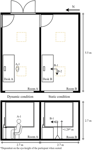
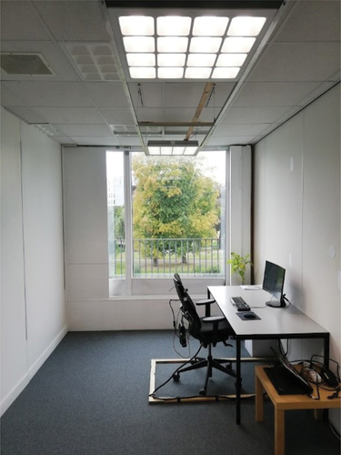
Fig. 2. Photograph of experimental room where the participant was located (room A).

Both rooms were 2.7 m x 5.5 m in size, 2.7 m in height and had a west-facing window of 1.7 m x 1.95 m with manually controlled blinds. The window provided view to the university campus. The view quality met the highest recommendation level according to EN17037 (CEN 2018) from the position of the participant. The blinds could be lowered by the experimenter, if the participant indicated that they perceived glare. The condition of the blinds was continuously logged to validate that the participants did not adjust them themselves.

Electric lighting was provided by two electric lighting fixtures (PHILIPS RC464B LED80S/TWH, CCT of 4500 K, suspended 0.3 m from the ceiling) in each room and was kept constant during the experiment. The average horizontal illuminance in the room due to electric light (without daylight) measured 0.8 m from the floor was 840 lx and the vertical illuminance 1.2 m from the floor at positions A-1 and B-1 was 230 lx. The mEDI due to electric lighting (without daylight) at the same vertical positions was 170 lx. The mean room temperature throughout the experiment was 23°C (st.d. = 1.5°C).

There was a desk in each room perpendicular to the window and a chair located 1.40 m from the window. The participant was facing north to avoid direct sunlight on their eyes. On each desk there was a computer screen (Samsung C24F390FHUXEN, 32.6 cm height, 54.8 cm width), a keyboard and a mouse. The computer screens in rooms A and B had the same brightness and the content of the screen used by the participant in room A was duplicated to the screen in room B. The screen luminance varied throughout the experiment as the participants used their computer (between 3 cd/m² for a fully black screen and 290 cd/m² for a fully white screen). A camera was placed on top of the screen facing the participant. The video from the camera was used to track face orientation (see section 2.5.1).

The movement of the participant’s chair had restrictions to ensure that the reference devices’ location matched the participant’s location. This restriction allowed participants to only slightly slide the chair forward or backward in order to stand up and sit again. At the start of the experiment, the participant adjusted the chair to their height. The height of the computer display was also adjusted, so that the line of sight of the participant fell between the middle and the top of the display when seated up straight. In room B, the height of the measuring equipment at positions B-1 and B-2 and the height of the computer screen were adjusted accordingly.

2.3. Participants

25 participants (13 female and 12 male) were recruited, through convenience sampling. All participants were students or employees of the Eindhoven University of Technology. Participants were included if, during an ordinary workday, they conducted work while seated at a desk and had a schedule from approximately 09:00 to 17:00. The age range was between 22 and 47 years (mean = 27.8, st.d. = 5.3). Their midpoint of sleep, corrected for sleep debt, (MSF_sc) was 4:15 ± 0:56 (hours: minutes), measured through the ultra-short version of the Munich Chronotype Questionnaire, µMCTQ (Ghotbi et al. 2020). The mean sleep quality score of the participants measured with the Groningen Sleep Quality Scale (Jafarian et al. 2008) was 4.2 ± 3.5 out of 14, indicating a good to average night of sleep before the experiment.

2.4. Protocol

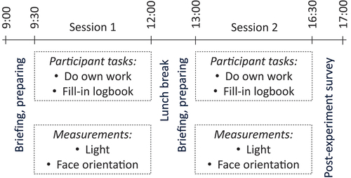
The participants were asked to bring their laptops or other (non-light emitting) equipment necessary to work while seated at a desk. The session started approximately at 8:30 in the morning with the participant entering room A and getting a brief introduction to the protocol of the study. The participants were not informed that their face orientation was investigated, to avoid biasing their behavior. They used the computer screen, keyboard, and mouse on desk A to connect to their laptop. The laptop was then placed underneath the desk. The use of smartphones in the experiment room was not allowed.

At 09:00, experiment session 1 (morning) started and the participant was asked to conduct their own work while seated at the desk and to keep track of their breaks in a logbook. A lunch break was scheduled from 12:00 to 12:45. During this break, the participants were allowed to leave the laboratory. After the lunch break the participants returned to the laboratory and started session 2 (afternoon) at 13:00. During session 2 the participants continued their own work, while still keeping track of their breaks in the logbook. Session 2 ended at 16:30 and was followed by a brief survey. The survey included questions about their experience with the experimental room, the presence of distractions, light perception and presence of glare. Since the experience of glare has been shown to affect viewing behavior (Sarey Khanie et al. 2017), a button connected to a logger was also placed on the desk in front of the participant, with which the participant could indicate the experience of glare. Glare was likely to be experienced on clear days toward the end of the experiment, due to direct sunlight shining onto the computer screen. The experimental data for the rest of the session after the glare indication were removed from analysis. During sessions 1 and 2, the participants were instructed to take breaks as needed inside or outside the laboratory, but report the time of break in the logbook. The protocol is displayed in Fig. 3. Approval for the study was obtained prior to the experiment by the Ethical Review Board of Eindhoven University of Technology (reference: ERB2022BE21).

Fig. 3. Experiment protocol.

2.5. Face orientation behavior

A person’s viewing direction consists of movements of the body, face and eyes (Sarey Khanie et al. 2017). For the purpose of this study only the first two components (movement of body and face) were included, due to difficulty of defining a valid field of view (FoV) that includes rotated eyes within the head. A person’s FoV is restricted by the eyelids, but as the eye rotates within the head the restriction changes (He et al. 2022; Zauner et al. 2023). This was not taken into account in this study. This sub-section describes how face orientation data were measured, corrected, cleaned and analyzed.

2.5.1. Measuring face orientation

The participants’ face orientation was tracked using the OpenFace 2.2.0 software (Baltrusaitis et al. 2016) that utilizes a video of the participant’s face captured with a webcam (logitech HD Webcam C615) on top of the computer screen in front of them. The software detects the face and identifies vertical face orientation (i.e., pitch or rotation of the head upwards or downwards) and horizontal face rotation (i.e., yaw or rotation of the head to the left or to the right). This software was used instead of wearable head-tracker to avoid overloading the participants’ head with equipment that could cause discomfort and restrict natural movement.

The FeatureExtraction program of the OpenFace software was used to get the face orientation of the participant. The accuracy of the face orientation tracking depends on the specification of the focal length and optical center coordinates of the camera. These camera parameters were calculated for the webcam using the OpenCV software (Bradski 2000).

2.5.2. Face orientation measurement correction

OpenFace has reported mean errors of 3.1 and 3.5 degrees in the calculation of horizontal and vertical face orientation angles respectively (Baltrusaitis et al. 2016). We performed our own validation of this by asking the participants to rotate their head horizontally to align their nose with marks on the wall indicating known angles. The mean difference of the OpenFace reported and the “real” horizontal face rotations was 8 degrees (st.d. = 6). This difference was larger for larger face rotation angles, with a linear relationship. Thus, the horizontal face rotation was corrected by a calibration factor, which was calculated by dividing the “real” angles with the OpenFace reported angles (1.22, average for all participants). The standard deviation over the participants was small (0.06), which allowed to use an average calibration factor.

2.5.3. Face orientation data cleaning

The face orientation data were cleaned before the analysis based on a few criteria. Data that corresponded to when participants had breaks (e.g., lunch break) were removed (13% of the collected face orientation data). The breaks were identified based on what participants reported at their logbooks.

Additionally, data that corresponded to when the blinds were closed were removed (2% of the collected face orientation data). Note that blinds were generally kept open, except if the participant requested to close them due to direct sunlight on their screen (this happened for part of two afternoons). During the experiment the blinds were lowered in both rooms A and B simultaneously, but it was decided to remove the data that corresponded to closed blinds due to uncertainty of how the change in view-out content would influence how much the participants looked toward outside. Since there were not enough data with lowered blinds, this influence could not be assessed.

Data during times when the participant experienced glare and pressed the glare button were also removed from the time that the button was pressed until the end of the experimental session (7% of the collected face orientation data). Specifically, 11 participants pressed the button in the afternoon after 15:00 when the direct sunlight was present and two participants pressed the button before 15:00. During one of the experiment days, the logger that recorded the glare button action failed. For that specific day, we checked the survey response of the participant to identify the occurrence of glare. The participant reported that glare was not experienced and therefore the data were kept. Finally, data were removed based on low confidence reported by OpenFace (11% of the collected face orientation data). Reported confidence more than 0.85 was considered reliable. Low confidence was generally reported when the participant’s face was not clearly visible. After applying the above data cleaning criteria, 67% of the OpenFace data were kept for analysis.

2.5.4. Data analysis of face orientation

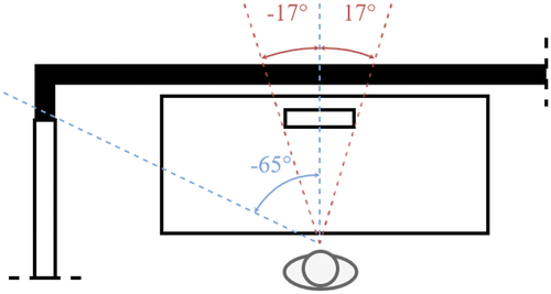
The distribution of face orientation was visualized for all participants combined in a 2D histogram with a bin size of 5 degrees. Mean, median and standard deviation of horizontal and vertical face rotation were computed. Since looking toward the window is expected to have the largest influence on the amount of light measured at eye-level, the mean, median and standard deviation of the duration of a face orientation toward the windows was computed. The duration of a face orientation toward positions with higher luminance (e.g., the window) is relevant in order to find out what light measurement interval is needed to capture the effect of face orientation. The participants’ face was directed toward the window when the horizontal face rotation was less than −65 degrees (negative values of face rotation are toward the direction of the window, Fig. 4). Data analysis was performed in python 3.8.

Fig. 4. Horizontal face rotation angles from the central view to the window and to the sides of the computer screen.

2.6. Measurement-based method

For the measurement-based method, the static and dynamic spectral irradiance were measured synchronously. Both mEDI and r_D were calculated from spectral irradiance data. This section describes the static and dynamic light measurements, additional light measurements in the space that were conducted to provide an overview of the experimental conditions, the light data correction, cleaning and analysis. The analysis is presented separately for the mEDI and the r_D data. Finally, an exploration of averaging data over larger intervals is presented.

2.6.1. Measuring static and dynamic light conditions

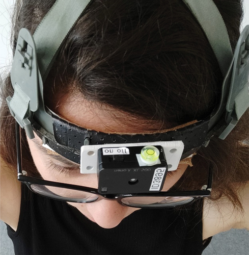
Spectral irradiance was measured with wearable spectrometers (NanoLambda BLE XL-500) attached to the participant’s head in room A (position A-1 in Fig. 1, dynamic condition) and toward the computer screen (positions B-1 in Fig. 1, static condition). Spectral irradiance was measured in the range from 390 to 760 nm with a step size of 5 nm. For position A-1, the spectrometer was attached to a helmet base that the participant was wearing on their head (Fig. 5).

Fig. 5. Wearable spectrometer placed on participant’s head.

During their breaks the participants placed the helmet with the spectrometer in a closed box. For position B-1 it was placed on a tripod whose height was adjusted in the morning of each day to the participants eye-level height. All measurements of spectral irradiance were collected with an interval of 2 seconds.

2.6.2. Additional light measurements

An additional fiber optics spectrometer (Ocean Optics USB4000) was placed in room B vertically toward the window (position B-2) on the tripod and collected data with an interval of 1 minute to be used as a reference. Two Raspberry Pi computers with an attached 180-degree fish-eye lens (Kruisselbrink et al. 2017) were placed at positions B-1 and B-2 and collected high dynamic range (HDR) images with an interval of 5 minutes. These images were collected to allow visual inspection of the experimental conditions if needed and to provide the luminance distribution.

2.6.3. Light measurement corrections

Two correction factors are applied to the light data: (i) a linear correction factor to both the static and dynamic conditions, and (ii) a room correction factor to the dynamic light condition.

2.6.3.1. Linear calibration of spectrometers

The two wearable NanoLambda spectrometers that were used to measure static and dynamic spectral irradiance were calibrated against a Konica Minolta CL500A spectrometer in an Ulbricht sphere with an incandescent light source in the mEDI range of 0 to 2500 lx. The mEDI was calculated from the spectral irradiance measurements. The melanopic linear calibration factors were calculated by dividing the mEDI from the Konica Minolta with the one from the wearable spectrometers (1.20 and 1.21 for the spectrometer used for the static and dynamic condition respectively, average over the range of measurements). The standard deviation over the range of measurements was small (0.01 and 0.02 for the spectrometer used for the static and dynamic condition spectrometer respectively), which allowed to use the average calibration factor per wearable spectrometer. The same calibration factors were applied to the effective irradiance input for the nvR_D model, since it has a linear relationship with mEDI (see subsection 2.1).

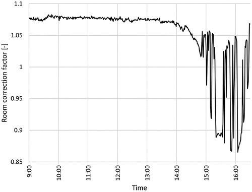
2.6.3.2. Room correction calibration

The two rooms (room A and B) inevitably slightly differ from each other. These differences were corrected by calculating a room correction factor. For this, baseline measurements were taken for one day without any participants present, with an interval of one minute (09:00–16:30 at 29 July 2022, which had a mix of clear, intermediate and overcast conditions). The electric lighting was set to the same levels that were used during the experimental sessions. The two wearable spectrometers were placed on tripods 1.2 m above the floor at positions A-1 and B-1, toward the computer screens. The room correction factor was calculated by dividing the mEDI at position B-1 with the mEDI at position A-1, after correcting both measurements with the previously described linear calibration factor.

The room correction factor was not constant throughout the day (as shown in Fig. 6). Large variation was observed at the end of the day when direct sunlight entered the room and reached the wearable spectrometers at large angles of incidence (from the side). The reason for this might be the poor directional response index of the wearable spectrometers (f₂ = 4.1% for mEDI, class C according to DIN [2016], calculation procedure described by Aarts et al. [2017]). To overcome this limitation of the equipment, we took the median of the correction factors measured throughout the day (1.07) instead of the mean which was skewed by the low values measured at the end of the day. It is expected that since data were removed after participants indicated that they experienced glare (which happened under clear sky conditions at the end of the experimental day) this limitation was mitigated to some extent.

Fig. 6. Factor indicating the difference in mEDI between the two rooms used in the experiment. Large variation is observed at the end of the day due to direct sunlight entering both rooms and the relatively poor directional response of the wearable spectrometers.

2.6.4. Light data cleaning

The data from the wearable spectrometers were cleaned before the analysis. As soon as one of the wearable spectrometers was saturated, data were removed from both the static and dynamic dataset (13% of the collected light data). The threshold for saturation was not constant because the data were collected with a variable integration time (i.e., the device automatically set the integration time based on the light level). Data were also removed during participants’ breaks (10% of the collected light data), usage of blinds (2% of the collected light data) and experience of glare (6% of the collected light data), similarly to what is described in subsection 2.5.3. After applying the above data cleaning criteria, 69% of the data collected by the wearable spectrometers were kept for analysis.

2.6.5. Data analysis of static and dynamic mEDI

To compare the static and the dynamic quantities we followed methods that are typically used for the comparison of simulated with measured quantities, which include visual analyses and hypothesis testing (Pierson et al. 2022). As previously mentioned, mEDI observations were collected every 2 seconds. The absolute difference for each observation (AD_i, 1), relative difference for each observation (RD_i, 2) and root mean square error for all N observations (RMSE, 3) between the mEDI of the static condition (mEDI_s,i) and mEDI of the dynamic condition (mEDI_d,i) were calculated. AD_i and RD_i provide information about the magnitude and direction of the difference, while RMSE is a measure of how concentrated the data are around the line of best fit.

Moreover, the relationship between the static and dynamic data was visually inspected through a scatter plot where each data point is color-coded by the horizontal face rotation (averaged within the 2-second interval that corresponds to the mEDI measurement). The color-coding allows for a visual inspection of how the face orientation affects the dynamic mEDI measurements. Since the mEDI and face orientation data needed to be synchronized to be plotted together, an additional 8% of the cleaned mEDI data and 2% of the cleaned face orientation data needed to be removed for this part of the analysis. The Pearson r between the mEDI_s,i and mEDI_d,i was calculated, to investigate the correlation between the two conditions. A certain degree of correlation is expected, since both conditions are affected similarly by the variations of daylight, but the correlation strength can indicate whether the effect of face orientation is large.

(1) $\mathit{A}{D}_i=\mathit{mED}{I}_{\mathit{s},\mathit{i}}-\mathit{mED}{I}_{\mathit{d},\mathit{i}}$(1)

(2) $\mathit{R}{D}_{\mathit{i}}=100\ast \left(\frac{\mathit{mED}{\mathit{I}}_{\mathit{s},\mathit{i}}-\mathit{mED}{I}_{\mathit{d},\mathit{i}}}{\mathit{mED}{I}_{\mathit{d},\mathit{i}}}\right)$(2)

(3) $\mathit{RMSE}=100\ast \sqrt{\left(\frac{1}{N}\right)\sum _{\mathit{i}=1}^N{(\frac{\mathit{mED}{\mathit{I}}_{\mathit{s},\mathit{i}}-\mathit{mED}{I}_{\mathit{d},\mathit{i}}}{\mathit{mED}{I}_{\mathit{d},\mathit{i}}})}^2}$(3)

Hypothesis testing was performed to test whether static and dynamic mEDI were significantly different from each other. However, since data were collected every 2 seconds, the resulting dataset had a very large number of observations (more than 200.000). This is bound to result to a very small p-value, without this being meaningful. For this reason, the averaged per participant mEDI for the static and dynamic condition were tested instead. A two-sided paired sample t-test was performed, since the assumption of normality was not violated (Shapiro-Wilk p = .79).

Since differences between participants might cancel each other out when using a simple t-test, it was further investigated whether the participant had a strong influence on the relationship between static and dynamic mEDI. To test this, a linear mixed model (LMM) was created with random slope for the effect of participant and was compared to a null linear model where participant was not included. The LMM was fitted using maximum likelihood estimation and the mEDI data were log-transformed to achieve model convergence (LMM formula in R notation: log₁₀ (mEDI_d) ~ log₁₀ (mEDI_s)+ (1 + log₁₀ (mEDI_s) | participant)). The significance of the random effect of participant was tested with a likelihood ratio test comparing the full LMM and null model. Visual inspection of the residuals did not reveal any discernible pattern and examination of the residual histogram indicated a distribution that appeared to be fairly normal.

All data analysis was performed in python 3.8, except the LMM analysis which was conducted in R 4.2.1 with the lme4 library (Bates et al. 2015).

2.6.6. Data analysis of static and dynamic r_D

The r_D was calculated using the Grasshopper plugin Lark 2.0 (Gkaintatzi-Masouti et al. 2022). Input to the model was the time series of spectral irradiance measured with the wearable spectrometers. The spectral irradiance was averaged over a 6-minute interval in order to be comparable with previous research that used the same model (Amundadottir 2016; Pierson et al. 2021, 2022). Effective irradiance was calculated from spectral irradiance and was processed by the functions of the model, using the Lark 2.0 Non-Visual Direct Response component. In this calculation, irradiance was used as a continuous time series of values, even though there were missing timesteps due to data cleaning (described in section 2.6.4). In addition, any light exposure prior to the start of the experiment was not considered.

The analysis of r_D was planned to follow similar steps as the analysis of mEDI. However, the results showed that this was not possible due to saturation of most responses. Therefore, only the distribution of static and dynamic r_D is presented.

2.6.7. Data averaging over larger intervals

Data from the spectrometers were collected with an interval of 2 seconds. Small measurement intervals are preferred for accurate light dosimetry (Hartmeyer et al. 2022). However, they might be impractical for daylight simulation applications due to the increase in simulation time, data load and lack of meteorological data with similar temporal resolution. Therefore averaging over larger periods was explored, using: 1) 1-minute intervals, which are often used in light dosimetry studies (Hartmeyer et al. 2022), 2) 6-minutes intervals, which are often used as input for the nvR_D model (Amundadottir 2016; Pierson et al. 2022), 3) 1-hour intervals, which are typical for annual simulations since meteorological data are usually available with this interval (Walkenhorst et al. 2002), 4) 8-hours intervals, as such averaging over the entire day for each participant. The RMSE and mean and standard deviation of the relative difference (RD_i) in mEDI were calculated for each of these intervals.

Averaging over the interval was preferred over taking its median since the former included differences caused by brief bright light episodes (e.g., a person momentarily looking toward the window). The rational for this is that studies that applied light pulses showed that even brief light episodes may initiate NIF responses (Joyce et al. 2022; Scheuermaier et al. 2010). Note that these studies typically use regular light pulses (i.e., constant duration of brief bright light followed by constant duration of darkness) in contrast to the irregular light pattern that one would obtain by occasionally looking toward the window. Nevertheless, taking an average over the interval can be seen as a worst-case scenario for the differences between static and dynamic light quantities (i.e., identifying the largest possible differences between the two conditions).

2.7. Simulation-based method

Since the limitations of the wearable light sensors might bias the difference found between the static and dynamic conditions, we implemented a second method using simulations. The mEDI for the static and dynamic conditions were simulated and compared. The measured face orientation data were used to simulate mEDI for the dynamic condition. This sub-section describes the process for simulating static and dynamic light conditions, the setup of the simulation model and the validation of the simulation model (i.e., comparison with measured light data).

2.7.1. Simulating static and dynamic light conditions

The simulation was performed for the days and time that the experiment took place (25 days in June-July 2022) for every minute in which face orientation data were available. Meteorological data collected at the location of the experiment were used to simulate static and dynamic mEDI in a virtual room identical to the experimental room (room B in Fig. 1).

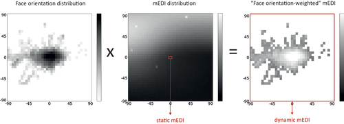
The mEDI for the static condition was simulated per minute for direction B-1 (always toward the computer screen, which is visually shown in Fig. 7). The mEDI for the dynamic condition was computed by combining the simulated light data for each minute with the face orientation data of the corresponding minute. The process of simulating the dynamic mEDI is graphically displayed in Fig. 8 and the steps are the following:

• The static view direction was rotated around the horizontal and vertical axes with a step of 5 degrees to create a matrix of directions (i.e., 37 different directions horizontally and vertically between −90 ° and + 90 ° with the static view as central direction). This matrix represents all possible face orientation directions of a participant with a sufficiently fine resolution (i.e., in total 37 × 37 = 1369 directions).

• For each direction, mEDI was simulated per minute.

• These mEDI values for each direction were multiplied with the fraction of time that the participant oriented their face toward that specific direction during the specific minute. This resulted in a “face orientation-weighted” mEDI for each direction.

• The dynamic mEDI was calculated as the sum of all these face orientation-weighted values per minute.

Fig. 7. Fish-eye view of the experimental room from the perspective of the camera measuring the static condition (direction B-1 in Fig. 1).

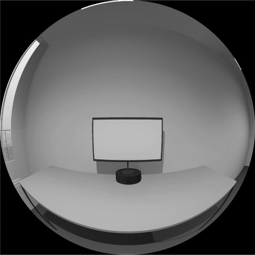
Fig. 8. Schematic process of simulating static and dynamic mEDI. The left image displays an example face orientation distribution during a minute and the middle image displays an example simulated mEDI distribution towards all possible face orientation directions for the corresponding minute. The two distributions are multiplied to produce a “face orientation-weighted” mEDI. Dynamic mEDI is calculated by adding up the “face orientation-weighted” mEDI matrix.

The mean absolute difference (AD_i, 1), mean relative difference (RD_i, 2) and root mean square error (RMSE, 3) between the simulated static and dynamic mEDI were calculated.

The simulation was performed using the Grasshopper plugins Lark 2.0 and Honeybee legacy 0.0.66 (Roudsari and Pak 2013) and the Radiance 5.4a simulation engine (Ward and Shakespeare 1998) (see Table 1 for the simulation parameters). Lark 2.0 was used to perform Climate Based Daylight Modelling (CBDM) with an increased spectral resolution. The model of the experimental room was created with Rhinoceros 3D (Robert McNeel & Associates 2023).

Table 1. Radiance simulation parameters.

Parameter	Value
ambient bounces (ab)	6
ambient divisions (ad)	10000
limit weight (lw)	0.0001

2.7.2. Simulation model setup

The necessary properties to create the simulation model are: 1) the spectral reflectance or transmittance of materials, 2) the direct normal irradiance (DNI) and diffuse horizontal irradiance (DHI) measured outside at an unobstructed point during the time of the experiment, 3) the luminous intensity distribution (through an ies file) and spectral power distribution (SPD) of the electric light and 4) the luminance emitted by the computer screen.

The surface reflectances were measured with the reflectance spectrometer (Konica Minolta CM-2600d, 10 nm spectral resolution) with and without specular reflections. Three to five measurements were taken and averaged for each surface. The specularity of each surface was calculated as the average percentage of specular reflections. The roughness of each surface was estimated visually according to recommended practice (Jakubiec 2021, 2022). The external ground surface was assumed to be green grass and its reflectance was taken from an online database (Jakubiec 2021). The obstructing trees were modeled with simplified geometry, as spectrally uniform translucent objects (Radiance material of type trans) with a transmittance of 0.2 and reflectance of 0.1 (Helliwell 2012). The glazing transmittance was measured with two spectrometers (Konica Minolta CL500-A, 1 nm spectral resolution) by taking paired measurements inside and outside of the window and dividing them. Measurements at different spots of the glazing were taken and averaged.

DNI and DHI were recorded every minute with a pyranometer (EKO MS-802/402 with a shadowball assembly MB-12-1), located on the roof of the Building Physics and Services laboratory of Eindhoven University of Technology. The sky spectral irradiance was measured using a fiber optics spectrometer located outside at an unobstructed point (EKO MS-711, 1 nm spectral resolution). It was averaged throughout all experimental days to be used as input to the simulation, since Lark cannot account for minutely variations in the spectral content of skylight. This was considered a reasonable simplification, based on findings from Pierson et al. (2022) that indicated that using constant sky spectrum was reasonably accurate in simulating mEDI in a room with neutral color surfaces for the location of Eindhoven.

The ies photometric file of the electric lighting fixtures was provided by the manufacturer. Since the luminaires were dimmed during the experiment, a dimming factor was applied in order to best match the measured vertical illuminance at positions B-1 and B-2. The SPD of the luminaires was measured directly under them with a spectrometer (Konica Minolta CL500-A).

The computer screen was modeled with a spectrally uniform and diffuse material of type glow. During the experiment, the screen luminance varied based on use. Since it was impractical to account for this variation in the simulation, a constant luminance of 150 cd/m² was used. This value was decided by randomly picking ten HDR images collected throughout the experiment at position B-1, obtaining the screen luminance for each and averaging them to a round value. Since the screen has only a minor contribution to the total vertical mEDI compared to the daylight and electric light in the room, this simplification is not expected to have a major influence on the result. The mean eye-level height of all participants (1.29 m) and the mean height of the computer screen above the desk (base of computer 7 cm above desk) was used for the simulation. The actual values varied among participants, but with small deviations (st.d. = 4 cm for the eye-level and st.d. = 2 cm for the computer base height).

2.7.3. Validation of the simulation model

The simulation model was compared with illuminances continuously measured vertically by the two spectrometers at positions B-1 and B-2. The mean relative error of the simulations against the measurements was −1% (1% for position B-1 and −4% for position B-2) and the RMSE was 47% (40% for position B-1 and 54% for position B-2). Although typically the relative error and RMSE are expected to be below 20%, previous research suggests that RMSE can be higher for vertical illuminance when simulating it through CBDM methods (similar to the simulation method used in this paper). Quek and Jakubiec (2021) have found an RMSE of 46% when comparing measurements and CBDM simulations of vertical illuminance in the field. In the current study, the higher RMSE was expected, since a few simplified assumptions were made for the simulation (the computer screen luminance has been modeled as constant, the mean eye-level height of all the participants and mean height of computer screen was used for the simulation). Since the mean relative error was low, the simulation model was considered good enough to be used for the analysis.

3. Results

This section presents the resulting face orientation distribution, followed by the results of the measurement-based and the simulation-based methods.

3.1. Face orientation results

Figure 9 displays the distribution of face orientation aggregated over all participants. The participants mostly oriented their face toward their computer screen (52% of the face orientations were concentrated in the central area within the black border of Fig. 9 and 86% within the area including an additional 8 degree error margin). The mean vertical face rotation was −2 degrees (median = −2, st.d. = 9). The mean horizontal face rotation was −3 degrees (median = −3, st.d. = 12).

Fig. 9. Face orientation distribution of all participants as a 2d histogram and boxplots of horizontal and vertical face rotation. Negative horizontal face rotation is towards the window. Negative vertical face rotation is downwards. The black dotted line indicates the location of the computer screen. The whiskers of the boxplots extend to 1.5 times the interquartile range. The red circle in the boxplots indicates the mean.

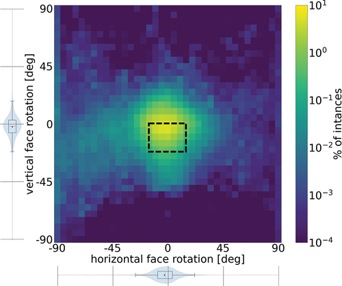
The mean duration of a face orientation toward the window was 4 seconds (median = 1, st.d. = 10). This short duration indicates that eye-level light data need to be measured with a small measurement interval in order to capture the effect of face orientation changes.

3.2. Measurement-based results

3.2.1. Results for mEDI

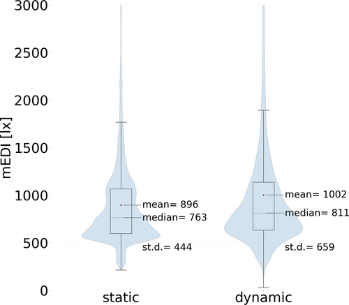
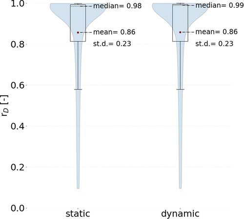
The distributions of both static and dynamic mEDI are presented in Fig. 10. The data with the 2-second measurement interval are presented, since the analysis of face orientation showed that duration of a face orientation toward the window tends to be short. The dynamic condition has a larger mean and median mEDI, as well as a larger standard deviation.

Fig. 10. Boxplots of measured static and dynamic mEDI (data collected with a 2-second sampling rate). The whiskers extend to 1.5 times the interquartile range. The red circle indicates the mean.

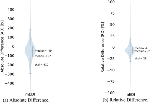
The distribution of absolute and relative difference in mEDI is displayed in Fig. 11a,b. The mean absolute and relative difference between the static and the dynamic mEDI is −107 lx and −4% respectively and the RMSE is 30%.

Fig. 11. Difference between measured static and the dynamic mEDI (data collected with a 2-second sampling rate). Negative values mean that the dynamic mEDI is larger than the static. The RMSE is 30%. The whiskers extend to 1.5 times the interquartile range. The red circle indicates the mean.

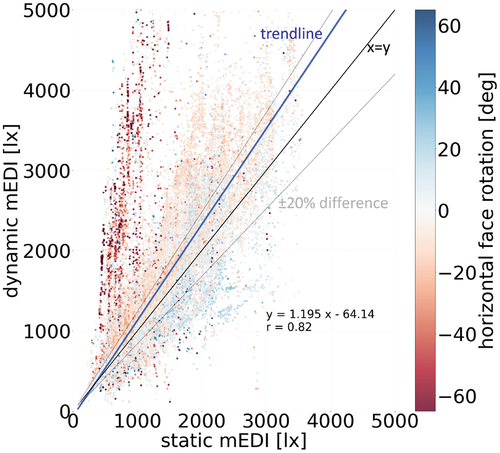
Figure 12 shows the scatter plot of the static and dynamic mEDI color-coded by the horizontal face rotation, including lines indicating a ± 20% relative difference (gray lines in the figure). 84% of the data are contained within the ± 20% lines, 10% of the data are above the top 20% line (which, as the mostly red color indicates, correspond mostly to participants facing toward the direction of the window) and 5% of the data are below the bottom 20% line (which, as the mostly blue color indicates, correspond to participants facing away from the window or part of the red-color data might correspond to facing downwards). The Pearson r is 0.82, indicating a strong correlation between the two conditions.

Fig. 12. Scatter plot of measured static versus dynamic mEDI (data collected with a 2-second sampling rate) color-coded by the horizontal head rotation (data averaged within 2 seconds). The static mEDI range is 210-3560 lx and the dynamic mEDI range is 30-11710 lx, but the plot is cropped to improve readability. The blue line is the trendline between the two (formula indicated on the figure). The thick black line is the x = y line and the grey lines are the ±20% relative difference limits.

The difference between the averaged per participant static and dynamic mEDI is statistically significant (two-tailed paired-sample t-test, t(24) = −5.62, p < 0.001). The LMM analysis including the effect of participant shows that a large fraction of the variance is explained by the random intercept (84% of the variance) and the random slope (10% of the variance) across participants. The likelihood ratio test results reveal a statistically significant difference between the full model and the null model (χ²(3) = 37055, p < 0.001), indicating that the inclusion of the random effect of participant improves the model fit. The model parameters of the full LMM are presented in Table 2.

Table 2. Model parameters of the full LMM.

Groups	Name	Variance	St.d.
Random effects:
Participant	(Intercept)	0.142	0.377
	log10 (mEDIs)	0.018	0.133
Residual		0.009	0.095
	Estimate	St. error	t value
Fixed effects:
(Intercept)	−0.104	0.076	−1.38
log10 (mEDIs)	1.047	0.027	39.36

3.2.2. Results for r_D

The distributions of both the static and dynamic r_D are presented in Fig. 13. The data averaged over 6 minutes are presented, since this is how this model is commonly used in literature. For both conditions most values are close to 1, which indicates that the response was saturated. The median values are close to 1 and more than 75% of the data are above 0.8. In subsection 4.2 we discuss possible explanations for this. This saturation means that further analysis of the r_D results is not meaningful.

Fig. 13. Boxplots of r_D for the static and dynamic condition (data averaged over 6-minute intervals). The whiskers extend to 1.5 times the interquartile range. The red circle indicates the mean.

3.2.3. Data averaging over larger intervals

Since the duration of face orientations toward the window was short, small measurement intervals are more relevant. Yet, they may be impractical. Here we present the results of how averaging over larger measurement intervals affects RMSE and RD_i (Fig. 14). Mean AD_i naturally remains constant (−107 lx).

Fig. 14. Relative difference (RD_i) between the measured static and dynamic mEDI (mean and standard deviation) and RMSE in relation to the measurement interval.

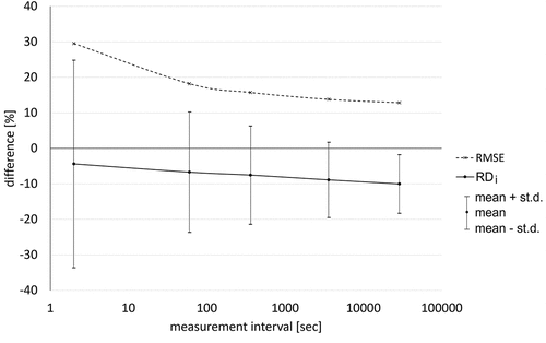
Averaging over intervals of 2 seconds, 1 minute, 6 minutes, 1 hour and 8 hours result in mean RD_i of −4%, −7%, −8%, −9% and −10% and RMSE of 30%, 18%, 16%, 14% and 13% respectively. Since RMSE is a measure of “noise” in the data, it naturally decreases as data are averaged over larger intervals (as does the standard deviation of RD_i). For intervals of 1 minute or more, both mean RD_i and RMSE are within a 20% limit. For intervals of 1 hour or more the RMSE saturates at approximately 13%.

3.3. Simulation-based results

The mean simulated mEDI for all face orientation directions is displayed in Fig. 15 and the distribution of simulated mEDI for the static and dynamic condition is displayed in Fig. 16. The mean simulated mEDI in the dynamic condition is 1013 lx, which is similar to the mean measured value (1002 lx, difference of 1%, see Fig. 10). The mean simulated mEDI in the static condition is 939 lx, which is also similar to the measured value (896 lx, difference of 5%, see Fig. 10). The mean AD_i in mEDI between the simulated static and dynamic condition is −74 lx (median = −40, st.d. = 175), whereas the mean RD_i is −6% (median = −5, st.d. = 13) and the RMSE is 15%.

Fig. 15. Simulated mean mEDI for all possible face orientations.

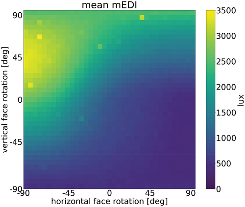
Fig. 16. Boxplots of simulated mEDI for the static and dynamic condition (data simulated per minute). The whiskers extend to 1.5 times the interquartile range. The red circle indicates the mean.

4. Discussion

This section discusses first the interpretation of the differences found between static and dynamic mEDI in order to put them in context. Next, the possible reasons for the saturation of the r_D results are discussed and finally the limitations of the study are presented.

4.1. Interpretation of mEDI results

The results showed a strong correlation between the static and the dynamic mEDI (Pearson r = 0.82), based on the recommendations of Ferguson (2009). The dynamic mEDI was larger than the static, but the difference between the two conditions was small (−107 lx or −4% according to the 2-second measured data, −74 lx or −6% according to the simulation per participant). This result is similar to the result of van Duijnhoven et al. (2019) that found that the dynamic luminous exposure was approximately 5% larger than the static. Although small, the difference between the static and dynamic mEDI averaged per participant is statistically significant, indicating that it is present on average.

The RMSE between static and dynamic mEDI for the 2-second data was 30% which is above the 20% limit that is generally considered acceptable (Mardaljevic 1995; Pierson et al. 2022). Yet, the comparison of the simulation model with measured vertical illuminance had a considerably larger RMSE (47%), which is in agreement with previous literature. Quek and Jakubiec (2021) argue that such deviations are acceptable as long as logarithmic differences are relatively small, since human vision is logarithmic (Reinhart and Andersen 2006). In their study they found that RMSE of vertical illuminance after applying a logarithmic transformation to their light data decreased to 7%, from 46% without the log-transformation. If a log10-transformation is applied to the 2-second mEDI data of the present study, the RMSE decreases to 3%. Based on the meta-analysis of Brown (2020), it seems that the relationship between mEDI and NIF effects is logarithmic, and therefore a log-transformation might be reasonable.

Moreover, averaging mEDI over larger intervals showed that RMSE (for the data without the logarithmic transformation) drops below the 20% limit for intervals of 1 minute or more. Recording intervals of less than 1 minute might be useful for light dosimetry studies. Other studies showed that intervals of 3 minutes or more cause loss in accuracy (Hartmeyer et al. 2022). It is unclear whether the smaller recording intervals can better predict NIF responses, but since bright light pulses might lead to NIF responses (Joyce et al. 2022; Scheuermaier et al. 2010) it could be relevant to record data with small intervals.

On the other hand, simulating light quantities for lighting design purposes with such small intervals is challenging. Weather data are typically available with an hourly resolution and even pyranometers rarely record data with a resolution of lower than 1 minute. Even if weather data were available, an annual simulation with a 2 second interval would result to 15.768.000 data points per simulated direction (in contrast to 8.760 data points from an hourly annual simulation). This large number of data would need to be aggregated in some way in order to create meaningful metrics for designers. This means that, while data collected with a 2-second interval are valuable for research purposes, they are unlikely to be used in lighting design simulations.

4.2. Interpretation of r_D results

Further analysis of the r_D results was not possible. The reason for this was that high light levels in the experiment room led to saturation of the model. The high light levels were a result of the mostly unobstructed view, the position of the participants near the window and the time of the year when the experiment was conducted. The measured light levels, although unusual for older buildings where there was less attention to daylight, might not be exceptional for modern office buildings. Yet, for positions further away from a window or for spaces with smaller daylight openings, our results might not be representative.

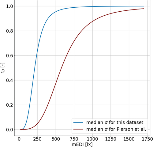
Figure 17 shows that at approximately 500 lx mEDI the alerting response becomes saturated. This was somewhat surprising, as a previous study that investigated the relationship between mEDI and r_D found that the response was saturated at 1500 lx mEDI (Pierson et al. 2022). As mentioned, the r_D calculation uses as input a time series of effective irradiance. The effective irradiance is smoothened by a simple moving average filter (SMA) to remove noise in the data. Then, it is parsed to a sigmoid function that converts it to alerting response using a half-saturation constant (σ) that is calculated for each timestep based on previous light history. Higher light history increases the σ, because if the NIF system is already adapted to high light levels it needs more light to have a response. In the study of Pierson et al. (2022) there are higher σ values compared to the present study due to differences in the previous light history. They report mEDI in a range of ~ 0–15.000 lx whereas in the present study most data are within ~ 100–4.000 lx. It is likely that, due to their generally higher light levels, more light is needed to initiate an alerting response (Fig. 18).

Fig. 17. Scatterplot of dynamic mEDI and dynamic r_D.

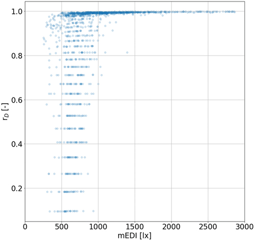
Fig. 18. Median intensity-response functions for the present dataset and the dataset collected by Pierson et al. (2022). A smooth time series of mEDI was inserted to the model to demonstrate the relationship between mEDI and r_D without the effect of the SMA filter.

The small difference between the static and the dynamic r_D might also be driven by the smoothing of the input effective irradiance data (by the SMA filter) and by the logarithmic transformation that this model applies which minimize the absolute differences in effective irradiance.

4.3. Limitations

In this study, we used in parallel a measurement-based method and a simulation-based method, that both have certain limitations. Therefore the combination of the two was necessary to obtain reliable results. Both methods point toward the same conclusion, but since small differences are found the limitations of the methods cannot be disregarded.

Since the static and dynamic conditions were measured in two different rooms, a room correction factor was applied to account for the small differences between the two (see subsection 2.6.3). As already mentioned, this correction factor might have been influenced by the accuracy of the wearable spectrometers. Given the small resulting difference between static and dynamic condition, this room difference might be important.

Face orientation was measured, which includes the movement of body and face, while eye movements were not considered. It is possible that eye movements might show larger deviations (e.g., people might quickly shift their eyes toward the window without rotating their head) and therefore the face orientation distribution is an underestimation of gaze distribution. However, measuring eye-centered light quantities presents practical difficulties. They cannot be measured by a wearable light sensor. They could potentially be simulated or measured with a combination of an eye-tracker and HDR images, as was done by Sarey Khanie et al. (2017), but defining a visual field that includes a rotated eye-in-head is difficult. Future studies could incorporate recently proposed dynamic FoV models that account for shifts in eye rotation (He et al. 2022).

Including the binocular FoV in the measurements and simulations might have been relevant, since it defines angles where light would never reach the eye. We conducted a further investigation to determine the influence of this limitation to the conclusions. Specifically, mEDI was simulated with and without a FoV restriction (based on Guth [1958]) for a direction facing the computer screen and one facing the window at eye-level height. In order to have a representative condition, daylight, electric light and light from the computer screen were included in the simulation and a point-in-time was selected where the mEDI toward the screen was similar to the mean static mEDI. This investigation showed that the FoV restriction reduced mEDI by approximately 20% for both directions (22% toward the computer screen and 19% toward the window). This shows that the FoV restriction has a large impact to the absolute mEDI that reaches the eye, which is in accordance with previous literature (Zauner et al. 2023). However, since the impact was similar to both directions the relative differences are not very large, which indicates that the comparison between static and dynamic mEDI would not likely lead to a different conclusion if a FoV restriction had been included.

The camera-based face-tracking method that was used has some limitations. As mentioned, a mean difference of 8 degrees between reference horizontal angles and the horizontal angles reported by OpenFace was found. A correction factor was applied based on this. However, part of the difference might be due to the difficulty of participants to align their head with the targets rather than OpenFace inaccuracy. The vertical rotation angles could not be corrected because visual inspection of the videos showed that participants were often aligning their eyes and not their head with the targets. Therefore, there was no reliable reference vertical rotation angle. Moreover, since the face detection is based on video recorded by a camera in front of the participant, it was not possible when the participants moved out of the FoV of the camera (e.g., when they bent their head too low). When that happened, a low detection confidence would be reported by OpenFace and the data would be removed (see 2.5.3). As mentioned, 11% of the face orientation data were removed due to low confidence. If we assume that a large proportion of these low confidence data happened when participants bent their head low on the desk (e.g., in order to write on paper), this might mean that the vertical face rotation was overestimated.

In addition, it is expected that most of the participants typically worked in an open-plan office, since they were recruited among students and employees of the university which consists mostly of this type of offices. It is likely that having a private office to work for a day led them to choose tasks that require more concentration, which is possibly related to facing more toward the computer screen. This means that the resulting face orientation distribution might be an underestimation of their natural face orientation behavior. Generally, in an open-plan office setup the situation might differ due to interactions with other people. These interactions were eliminated in the current experiment but it would be useful to explore their effect in a future experiment.

Previous research has indicated that luminance distribution can affect where people face (Sarey Khanie et al. 2017; Vincent et al. 2009). In this study, this was not explicitly investigated, but a valid question would be whether people face more toward the window when it is brighter, and therefore a more pleasant view, or less to avoid glare. As already mentioned, glare was eliminated from the measured data and is therefore unlikely to have had an effect. But since the effect of window luminance on face orientation might be of interest, we conducted an additional investigation. Specifically, we compared vertical illuminance toward the window when a participant was facing the window with vertical illuminance toward the same direction at all other times during the experiment. Only very small differences in vertical illuminance were observed (mean vertical illuminance with face orientation to window = 3811 lx, median = 3503 lx, while mean vertical illuminance without face orientation to window = 3880 lx, median = 3478 lx). Based on this, it seems that there might have been reasons other than luminance that led people to face the window, for example need for restoration or people walking outside. This could be further investigated in a future study.

5. Conclusion

This paper presented the results of a semi-controlled laboratory experiment that investigated the difference between the actual dynamic eye-level light conditions of office workers and the light conditions measured statically toward a computer screen. The participants were free to perform their typical office tasks, while their face orientation and dynamic eye-level light was tracked. A measurement-based and a simulation-based method were used in parallel.

The measurement-based method showed that the dynamic mEDI was 4% to 10% larger than the static, depending on the measurement interval. This difference was statistically significant for data averaged per participant. A similar difference was found through the simulation-based method (dynamic mEDI 6% larger than static). The correlation coefficient between static and dynamic mEDI was strong (0.82) and for 84% of the data the difference between the two quantities was within a 20% limit. Differences in relative alerting response (r_D) could not be investigated, since most responses for both the static and dynamic condition were saturated due to generally high light levels in the experimental room.

The dominant face orientation of the participants was toward the computer screen, where 52% of the face orientations were concentrated (which was 86% if an additional 8 degree margin is included). The mean vertical face rotation was −2 degrees (downwards) and the mean horizontal face rotation was −3 degrees (toward the window). The mean ±standard deviation of the horizontal and vertical face rotations were within 15 degrees from the center.

The results show that measuring and simulating personal light conditions of office workers statically toward a computer screen might be an underestimation of their actual eye-level light conditions, although this underestimation is relatively small. Considering that there are uncertainties in both measurements and simulations that could explain the resulting difference, it seems that including dynamic face orientation in office lighting design is not a priority. Since this study was performed in a single-user office with few distractions, a follow-up study in an open-plan office is useful in order to obtain more ecologically valid results.

Acknowledgments

The authors would like to thank Sietse de Vries for conducting a pilot experiment that helped refine the methodology of the current one and for sharing his figures.

Disclosure statement

No potential conflict of interest was reported by the author(s).

Data availability statement

The data that support the findings of this study are available online and can be accessed here: https://doi.org/10.5281/zenodo.11483059.

Additional information

Funding

This work was supported by the European Training Network LIGHTCAP under the Marie Skłodowska- Curie actions framework H2020-MSCA-ITN-2019 [grant number 860613].

References

- Aarts MPJ, van Duijnhoven J, Aries MBC, Rosemann ALP. 2017. Performance of personally worn dosimeters to study non-image forming effects of light: assessment methods. Build Environ. 117:60–72.
- Abboushi B, Safranek S. 2022 Jul 18–21. Determining critical points to control electric lighting to meet circadian lighting requirements and minimize energy use. Proceedings of Annual Modeling and Simulation Conference (ANNSIM); San Diego (CA), USA. p. 559–568.
- Adamsson M, Laike T, Morita T. 2019. Comparison of static and ambulatory measurements of illuminance and spectral composition that can be used for assessing light exposure in real working environments. LEUKOS - J Illuminating Eng Soc North Am. 15(2–3):181–194.
- Altenberg Vaz N, Inanici M. 2020. Syncing with the sky: Daylight-driven circadian lighting design. LEUKOS - J Illuminating Eng Soc Of North Am. 17(3):291–309. doi: 10.1080/15502724.2020.1785310.
- Amundadottir ML. 2016. Light-driven model for identifying indicators of non-visual health potential in the built environment [ Doctoral dissertation]. Lausanne (Switzerland): Ecole Polytechnique Federale de Lausanne.
- Baltrusaitis T, Robinson P, Morency LP. 2016 Mar 7–10. OpenFace: an open source facial behavior analysis toolkit. Proceedings of IEEE Winter Conference on Applications of Computer Vision; Lake Placid (NY), USA. p. 1–10.
- Bates D, Machler M, Bolker B, Walker S. 2015. Fitting linear mixed-effects models using lme4. J Stat Softw. 67(1):1–48.
- Bradski G. 2000. The OpenCV library. Dr Dobb’s J Software Tools. 120:120–125.
- Brennan MT, Collins AR. 2018 Sep 26–28. Outcome-based design for circadian lighting: an integrated approach to simulation & metrics. Proceedings of ASHRAE and IBPSA-USA Building Simulation Conference; Chicago (IL), USA. p. 141–148.
- Brown TM. 2020. Melanopic illuminance defines the magnitude of human circadian light responses under a wide range of conditions. J Pineal Res. 69(1):e12655.
- Brown TM, Brainard GC, Cajochen C, Czeisler CA, Hanifin JP, Lockley SW, Lucas RJ, Münch M, O’Hagan JB, Peirson SN, et al. 2022. Recommendations for daytime, evening, and nighttime indoor light exposure to best support physiology, sleep, and wakefulness in healthy adults. PLOS Biol. 20(3):e3001571.
- [CEN] European Committee for Standardization. 2018. Daylight in buildings (EN 17037:2018). Brussels (Belgium): CEN.
- [CIE] International Commission on Illumination. 2018. System for metrology of optical radiation for ipRGC-influenced responses to light (CIE S 026/E:2018). Vienna (Austria): CIE.
- [DIN] Deutsches Institut für Normung. 2016. Photometry-Part 7: classification of illuminance meters and luminance meters (DIN 5032-7:2016-06). Berlin (Germany): DIN.
- Ferguson CJ. 2009. An effect size primer: a guide for clinicians and researchers. Prof Psychol Res Pr. 40(5):532–538.
- Ghotbi N, Pilz LK, Winnebeck EC, Vetter C, Zerbini G, Lenssen D, Frighetto G, Salamanca M, Costa R, Montagnese S, et al. 2020. The µMCTQ: an ultra-short version of the Munich Chronotype questionnaire. J Biol Rhythms. 35(1):98–110.
- Gkaintatzi-Masouti M, Pierson C, van Duijnhoven J, Andersen M, Aarts MPJ. 2022. A simulation tool for building and lighting design considering ipRGC-influenced light responses. Web Of Conf. 362:01001. doi: 10.1051/e3sconf/202236201001.
- Guth SK. 1958. Light and comfort. Ind Med Surg. 27(11):570–574.
- Hartmeyer SL, Webler FS, Andersen M. 2022. Towards a framework for light- dosimetry studies: methodological considerations. Lighting Res Technol. 55(4–5):337–399. doi: 10.1177/14771535221103258.
- He S, Li H, Yan Y, Cai H. 2022. Capturing luminous flux entering human eyes with a camera, Part 1: fundamentals. LEUKOS - J Illum Eng Soc North Am. 1–19. doi: 10.1080/15502724.2022.2147942.
- Helliwell R. 2012. Site layout planning for daylight and sunlight: a guide to good practice. Arboric J. 34(1):52–54. doi: 10.1080/03071375.2012.692505.
- Houser K, Boyce PR, Zeitzer JM, Herf M. 2021. Human-centric lighting: myth, magic or metaphor? Lighting Res Technol. 53(2):97–118.
- Jafarian S, Gorouhi F, Taghva A, Lotfi J. 2008. High-altitude sleep disturbance: results of the Groningen sleep quality questionnaire survey. Sleep Med. 9(4):446–449.
- Jakubiec JA. 2021. Spectral materials database. [accessed 2023 Nov 30]. http://spectraldb.com/about.html.
- Jakubiec JA. 2022. Data-driven selection of typical opaque material reflectances for lighting simulation. LEUKOS - J Illum Eng Soc Of North Am. 19(2):176–189. doi: 10.1080/15502724.2022.2100788.
- Joyce DS, Spitschan M, Zeitzer JM. 2022. Optimizing light flash sequence duration to shift human circadian phase. Biology. 11(12):1807.
- Khademagha P, Aries MBC, Rosemann ALP, van Loenen EJ. 2016. Implementing non-image-forming effects of light in the built environment: a review on what we need. Build Environ. 108:263–272.
- Knoop M, Broszio K, Diakite A, Liedtke C, Niedling M, Rothert I, Rudawski F, Weber N. 2019. Methods to describe and measure lighting conditions in experiments on non-image-forming aspects. LEUKOS - J Illum Eng Soc Of North Am. 15(2–3):163–179.
- Konis K. 2019. A circadian design assist tool to evaluate daylight access in buildings for human biological lighting needs. Sol Energy. 191:449–458.
- Kruisselbrink T, Aries M, Rosemann ALP. 2017. A practical device for measuring the luminance distribution. Int J Of Sustainable Lighting. 19(1):75–90. doi: 10.26607/ijsl.v19i1.76.
- Mardaljevic J. 1995. Validation of a lighting simulation program under real sky conditions. Lighting Res Technol. 27(4):181–188.
- Pierson C, Aarts MPJ, Andersen M. 2022. Validation of spectral simulation tools in the context of ipRGC-influenced light responses of building occupants. J Build Perform Simul. 16(2):179–197. doi: 10.1080/19401493.2022.2125582.
- Pierson C, Soto Magan VE, Aarts MPJ, Andersen M. 2021. A conceptual simulation workflow to guide design decisions regarding the effects of daylight on occupants’ alertness. J Phys Conf Ser. 2042(1):012116. doi: 10.1088/1742-6596/2042/1/012116.
- Potocnik J, Kosir M. 2020. Influence of commercial glazing and wall colours on the resulting non-visual daylight conditions of an office. Build Environ. 171:106627.
- Quek G, Jakubiec JA. 2021. Calibration and validation of climate-based daylighting models based on one-time field measurements: office buildings in the tropics. LEUKOS - J Illuminating Eng Soc Of North Am. 17(1):75–90.
- Reinhart CF, Andersen M. 2006. Development and validation of a radiance model for a translucent panel. Energ Buildings. 38(7):890–904.
- Robert McNeel & Associates. 2023. Rhinoceros 3D. [accessed 2023 Nov 30]. https://www.rhino3d.com/.
- Roudsari MS, Pak M. 2013 Aug 15–28. Ladybug: A parametric environmental plugin for grasshop- per to help designers create an environmentally-conscious design. Proceedings of 13th Conference of the International Building Performance Simulation Association; Chambery (France). p. 3128–3135.
- Sarey Khanie M, Stoll J, Einhauser W, Wienold J, Andersen M. 2017. Gaze and discomfort glare, part 1: development of a gaze-driven photometry. Lighting Res Technol. 49(7):845–865.
- Scheuermaier K, Laffan AM, Duffy JF. 2010. Light exposure patterns in healthy older and young adults. J Biol Rhythms. 25(2):113–122.
- Soto Magan VE. 2021. Alertness in work environments - on the role of indoor daylight exposure [ Doctoral dissertation]. Lausanne (Switzerland): ecole Polytechnique Federale de Lausanne.
- Spitschan M, Stefani O, Blattner P, Gronfier C, Lockley S, Lucas R. 2019. How to report light exposure in human chronobiology and sleep research experiments. Clocks & Sleep. 1(3):280–289.
- van Duijnhoven J, Aarts MPJ, Kort HSM. 2019. The importance of including position and viewing direction when measuring and assessing the lighting conditions of office workers. Work. 64(4):877–895.
- Vetter C, Pattison PM, Houser K, Herf M, Phillips AJK, Wright KP, Skene DJ, Brainard GC, Boivin DB, Glickman G. 2021. A review of human physiological responses to light: implications for the development of integrative lighting solutions. LEUKOS - J Illuminating Eng Soc Of North Am. 18(3):387–414. doi: 10.1080/15502724.2021.1872383.
- Vincent BT, Baddeley R, Correani A, Troscianko T, Leonards U. 2009. Do we look at lights? Using mixture modelling to distinguish between low- and high-level factors in natural image viewing. Vis cogn. 17(6–7):856–879.
- Walkenhorst O, Luther J, Reinhart C, Timmer J. 2002. Dynamic annual daylight simulations based on one-hour and one-minute means of irradiance data. Sol Energy. 72(5):385–395.
- Ward G, Shakespeare R. 1998. Rendering with Radiance: the art and science of lighting visualization. San Fransisco (USA): morgan Kaufmann Publishers, Inc.
- Zauner J, Broszio K, Bieske K. 2023. Influence of the human field of view on visual and non-visual quantities in indoor environments. Clocks & Sleep. 5(3):476–498.
- Zeng Y, Sun H, Lin B. 2021. Optimized lighting energy consumption for non-visual effects: a case study in office spaces based on field test and simulation. Build Environ. 205:108238.