Measuring autophagosome flux

ABSTRACT

Macroautophagy/autophagy is a proteolytic pathway that is involved in both bulk degradation of cytoplasmic proteins as well as in selective degradation of cytoplasmic organelles. Autophagic flux is often defined as a measure of autophagic degradation activity, and many techniques exist to assess autophagic flux. Although these techniques have generated invaluable information about the autophagic system, the quest continues for developing methods that not only enhance sensitivity and provide a means of quantification, but also accurately reflect the dynamic character of the pathway. Based on the theoretical framework of metabolic control analysis, where the autophagosome flux is the quantitative description of the rate a flow along a pathway, here we treat the autophagy system as a multi-step pathway. We describe a single-cell fluorescence live-cell imaging-based approach that allows the autophagosome flux to be accurately measured. This method characterizes autophagy in terms of its complete autophagosome and autolysosome pool size, the autophagosome flux, J, and the transition time, τ, for autophagosomes and autolysosomes at steady state. This approach provides a sensitive quantitative method to measure autophagosome flux, pool sizes and transition time in cells and tissues of clinical relevance.

Abbreviations: ATG5/APG5, autophagy-related 5; GFP, green fluorescent protein; LAMP1, lysosomal-associated membrane protein 1; MAP1LC3/LC3, microtubule-associated protein 1 light chain 3; J, flux; MEF, mouse embryonic fibroblast; MTOR, mechanistic target of rapamycin kinase; nA, number of autophagosomes; nAL, number of autolysosomes; nL, number of lysosomes; p-MTOR, phosphorylated mechanistic target of rapamycin kinase; RFP, red fluorescent protein; siRNA, small interfering RNA; τ, transition time; TEM, transmission electron microscopy.

KEYWORDS:

• Autophagosome flux
• autophagy
• fluorescence microscopy
• steady-state
• transition time

Introduction

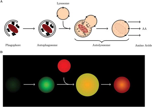
Autophagy (from Greek auto, ”self” and phagein, ”to eat”) is an evolutionary conserved highly dynamic and flexible process that involves both the bulk degradation of cytoplasmic proteins as well as the selective degradation of cytoplasmic organelles [1]. Autophagy plays an essential role in maintaining cellular integrity by preventing the buildup of potentially toxic or damaging proteins and organelles. It involves the sequestration of cytoplasmic materials in a vesicle known as an autophagosome, and the concomitant delivery thereof into lysosomes for the degradation and recycling of the digested goods (Figure 1(a)). Over the last decade our understanding of the autophagy machinery, especially the mammalian system, has greatly advanced. We know that this degradative pathway serves as a means to revitalize the intercellular protein pool, to remove deleterious proteins and organelles, and to contribute to the function of the innate immune response [2]. Therefore it is not surprising that deterioration in the degradative capacity of autophagy has profound implications for cell metabolism and proteostasis. This is most evident in, for example, neurodegeneration where there is a gradual loss in autophagic degradation function accompanied with the build-up of toxic protein aggregates and the subsequent death of neuronal cells [2]. It is the dual role of autophagy, both in cell protection and disease progression, that has led to growing interest in the assessment of the complete system and its dynamics.

Figure 1. The process of macroautophagy. (a) Schematic representation of the autophagic process, and (b) cartoon illustration of the fluorescence signal of a cell expressing GFP-LC3B and stained with LysoTracker Red.

Autophagic flux is generally defined as a measure of the autophagic system’s degradation activity [3]. Although a number of approaches are currently used to assess autophagic flux, many have inherent shortcomings. Western blot analysis, for example, allows for the indirect assessment of the number of autophagosomes based on the abundance of MAP1LC3/LC3-II protein in the presence and absence of a fusion inhibitor such as bafilomycin A1 (BAF), from which one can infer whether or not autophagic flux has increased, or decreased. The major challenge when using western blot analysis in this context is the fact that it does not measure a rate [4]. Furthermore, western blot analysis is also plagued with technical challenges such as high variability and difficulty in accurately assessing small changes in LC3-II levels. Transmission electron microscopy (TEM), considered as the gold standard in many autophagy research applications, has the advantage of allowing a direct assessment of autophagosomes in cells. However, unless TEM tomography is performed in combination with morphometrics it only allows for the partial analysis of the autophagosome pool size [5]. TEM also requires cells to be fixed, which prevents the assessment of autophagosomes over time, a requirement for determining autophagic flux. Fluorescence microscopy can be used for both live cell imaging and optical sectioning through the whole cell to measure the complete autophagosome pool in a single cell over time. If such an assessment is not performed over time with appropriate fusion inhibitors, it cannot describe autophagic flux, because there is no time dimension that allows for the expression of a rate.

There have been a few techniques that have been successfully implemented to infer whether or not there is autophagic flux. These include the use of the mCherry-LC3 transgenic mouse model [6] and photo-activatable fluorescent probes [7]. The greatest hurdle faced by current techniques is that they are less suitable for the measurement of autophagic flux as a rate. In order to accurately measure the autophagic flux (or, more accurately, the autophagosome flux) the assessment of the complete autophagosomal pool size over time is required to calculate flux from the dynamic changes in pool size in the presence and absence a autophagosome and lysosome fusion inhibitor. We have previously described an approach of defining and measuring autophagosome flux, where we treat the autophagic process as a multistep pathway with each individual step characterized by a particular rate [8]. Based on the metabolic control analysis approach, we have reserved the term flux (J) for the steady-state rate of flow along a metabolic pathway. It is possible to measure the flux of a pathway by completely inhibiting one of the steps in the pathway at steady state, when all individual rates are equal, and from the initial rate of increase in substrate of the inhibited step to calculate the flux, J, as well as the transition time, τ. We made the distinction between the autophagosome flux, i.e., the rate of flow along the vesicular pathway, and the flux of substrate clearance, indicating the rate of cargo degradation within the vesicular system. Here we present a detailed protocol to measure autophagosome flux. This approach relies on the dynamic assessment of the number of autophagosomes (nA), autolysosomes (nAL) and lysosomes (nL) over time in a single cell.

The protocol described here makes use of cells that stably express green fluorescent protein tagged to LC3 (GFP-LC3), which makes autophagosomes visible as green puncta because LC3 is a structural component of autophagosomes. The addition of a LysoTracker Red fluorescent probe allows the visualization of acidic vesicles, lysosomes, as red puncta. The co-localization of green and red fluorescence signal indicates the presence of autolysosomes, because GFP is not immediately degraded when autophagosomes fuse with lysosomes. Initially autolysosomes fluoresce yellow and slowly transition to red emitted light as the GFP is being degraded (Figure 1). The protocol here described will include instructions how to quantify the complete autophagosome (nA), autolysosome (nAL) and lysosome (nL) pool size in a single cell over time using a micropattern approach, to determine (i) whether or not the autophagic system is in steady state, (ii) to measure the steady-state variables and, (iii) to determine the autophagosome flux, J, as well as the transition time τ. In the discussion section we will compare the here describe method with those described previously and comment on the autophagic variables derived from our approach as well as their potential use. Finally, we provide an example data set generated in a candidate cell type using the protocol described and characterize basal as well as rapamycin-induced autophagy in terms of its steady-state variables and autophagosome flux.

Materials

Cell culture

1. Mouse embryonic fibroblast (MEF) cells stably expressing GFP-LC3B protein.

2. Dulbecco modified Eagle medium (DMEM) (Life Technologies, 41–965-039) supplemented with 10% fetal bovine serum (Biochrom, S-0615) and penicillin-streptomycin (Life Technologies, 15–140-122).

3. General tissue culture apparatus used to culture and maintain cells.

Microscopy

Microscopy

1. CYTOO micro-patterned slides with large fibronectin disc shapes (CYTOO, 10–003-10).

2. CYTOO life chamber dish (CYTOO, 30–010).

3. Olympus IX81 wide-field microscope (Hamburg, Germany) suited for live cell imaging that is equipped with an automated z-stack and stage control.

Software

1. Cell R.

2. ImageJ (http://rsbweb.nih.gov/ij/download.html) with modified WatershedCounting3D plug-in [9].

Chemicals

1. Bafilomycin A1 (BAF) (LKT Laboratories Inc., B-0025).

2. Rapamycin (Sigma-Aldrich, R-0395).

3. LysoTracker Red (Thermo Fisher, L-7528).

4. LysoTracker Blue (Thermo Fisher, L-7525).

5. Lipofectamine 3000 transfection kit (Thermo Fisher, L-300–0008).

6. Atg5/Apg5 FlexiTube siRNA (Qiagen, SI-0263–3946)

Methods

In brief, cells were cultured and prepared for live cell imaging, and intracellular autophagosomal, autolysosomal and lysosomal pool sizes were assessed over time. Following the complete inhibition of fusion between autophagosomes and lysosomes, the autophagosome flux was determined.

Preparations

Preparation of cells for microscopy

1. Seed the cells in a flask containing culture media and incubate in a humidified atmosphere in the presence of 5% CO2 at 37◦C. Once the cells have reached 80% confluency, proceed to harvest cells by trypsinisation, seed the cells into a new flask and incubate so that the cells can reach their log growth phase. Note: at this point cells can be transfected with fluorescence tags, such as GFP-Lc3b and RFP-Lamp1, or with Atg5 siRNA, as a negative control. Lipofectamine 3000 was used to silence Atg5 with Atg5/Apg5 FlexiTube siRNA.

2. When the culture has reached 80% confluence, harvest cells by trypsinisation and seed the cells into the CYTOO chamber dish containing the micropatterned slide with culture media (see note 2 in the notes section for detailed information about the micro-patterned slides).

3. Leave the cells to settle and attach for 30 min and rinse with culture media until all remaining cells are washed off from the non-fibronectin patterned areas of the slide.

4. Refresh culture media containing 75 nM LysoTracker Red. Leave cells to equilibrate for 2 h and then use for microscopy.

Live cell imaging set-up

1. Calibrate the stage control of the fluorescent microscope stage.

2. Maintain the culture chamber environment of the microscope stage at 37◦C with 5% CO2 in a humidified atmosphere.

3. Using the experimental planner, usually part of the microscope imaging software, set up the imaging protocol.

   1. Focus on a single cell with x100 oil immersion objective using a weak trans-illumination (white light) setting.

   2. Use the live streaming function (live camera) to display the cell on the screen as the image would be captured. Switch to fluorescence using the filter and illumination control panel, set the excitation filter to 492 nm (for green channel) with an appropriate emission filter (UBG or GFP). Tune the light intensity and exposure so that an optimal signal/noise ratio is achieved, while minimizing phototoxicity (see note 5 in notes section).

   3. Repeat the above step for the red fluorescence channel by setting the excitation filter to 572 nm with an appropriate emission filter (e.g. UBG triple bandpass).

   4. Set the experimental planner for z-stack imaging so that there is multiple channel (red and green) acquisition per z-plane. Set the light intensity and exposure time to the values determined in the previous 2 steps in the experimental planner to provide optimal signal/noise ratio when executing the acquisition protocol. Note: The z- stack plane parameters (the position of the top and bottom plane) will not be defined here, because it will be set individually for each cell prior to image acquisition.

4. Find candidate cells and record their x,y positions using the microscope stage control panel. This can be done by either trans-illumination or fluorescence; it is important to use the lowest intensity possible to avoid photo-bleaching of fluorochromes.

5. Allow the cells to equilibrate for 1 h (because the previous steps expose cells to high energy light and can lead to a stress response if exposed for a longer period of time).

6. Using the stage control panel move to the first (or desired) cell.

7. Use the live streaming function (live camera) to display the cell on the screen as it would be captured, and determine the bottom plane of the cell (the lowest z plane point) and set it as the plane at which the first image will be captured in the z-stack series. Then move the focal plane to the highest point of the cell where autophagosomal, autolysosomal and lysosomal structures are still observed and set it as the top plane (the highest z-plane image frame) for the image stack to be acquired. Set the step width between frames to 500 nm and the software will automatically set the number of image frames between the top and bottom plane to achieve an increment of 500 nm between image frames.

8. Execute the experimental protocol to acquire the z-stack image.

9. Using the stage control in step 6 navigate to the next cell, and image as described in step 7 and 8. Continue until all cells have been imaged. A minimum number of 10 to 30 cells is recommended to achieve sufficient statistical power (see note 9 in notes section).

Image analysis

1. Process image stacks using 3D deconvolution.

2. Adjust contrast and color brightness (if necessary) to improve signal/noise ratio. Be sure to maintain pixel values within the measurable range.

3. Display image stack (with both green and red channels) as a maximum intensity projection and, using the “click count” function, count the only the green puncta (autophagosomes), and then the red puncta (lysosomes).

4. Export processed image stack consisting only of the green or red channel as a tiff file.

5. Open tiff image using ImageJ.

6. Run WatershedCounting3D using parameters that allow optimal discrimination of signal/background and record the puncta count for the respective channels.

7. Calculate the autolysosomal value by subtracting the autophagosomal value, obtained in step 3, from the total puncta count determined using the green channel image stack. Note: this value should be similar to the number of total red puncta minus the lysosomal count.

Measuring autophagosome flux at the single-cell level

Determine the concentration of fusion inhibitor required for the complete inhibition of autophagosome and lysosome fusion

1. Prepare cells and set up the imaging protocol as described in section 4.1.1 and 4.1.2 (steps 1 to 5).

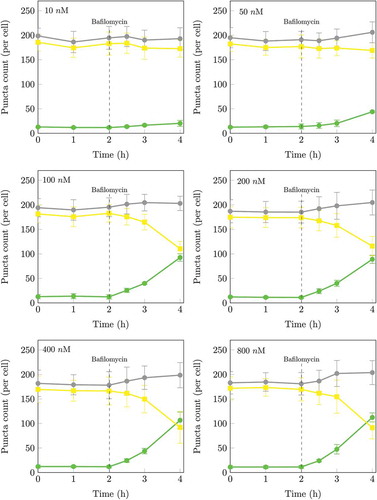
2. Verify that the autophagic system is in a steady state. Image cells every hour as described in section 4.1.2 steps 6 and 9, and quantify the number of autophagosomes (nA), autolysosomes (nAL) and lysosomes (nL) per cell per as described in section 4.1.3 over a period of time for at least 3 time points under control conditions without the presence of fusion inhibitors or drugs. When nA remains constant over time, it signifies that the system is in a steady state in which the rate of autophagosome synthesis equals the rate of autophagosome degradation. If nA changes over time the autophagic system is in a transition state; continue to monitor nA until it remains constant. Figure 2 shows that the nA and nAL per cell remains constant over time (0 to 2 h) under basal conditions indicating that the autophagic system is in steady state. Note: there will be minor variations in nA over time at steady state as the system does exhibit stochastic behavior; use the average nA to determine whether the system is in steady state.

3. Next treat cells with a series of increasing concentrations of Bafilomycin A1 (BAF). Acquire images (section 4.1.2, steps 6 to 9) and quantify (section 4.1.3) nA and nAL with a minimum of 3 to 5 time points following inhibition at 30-min intervals.

4. The concentration of fusion inhibitor required for the complete inhibition of fusion is reached when there is no further increase in the initial rate of autophagosome (nA) accumulation per cell with increasing fusion inhibitor concentration. Figure 2 shows the effect of saturating concentrations of BAF on the rate of autophagosome accumulation. Note, incomplete fusion inhibition will result in a residual autophagosome flux, which jeopardizes subsequent accurate flux assessment.

5. Because this experiment is performed under basal conditions, the basal autophagosome flux, Jbasal, is the initial slope of the progress curve of the autophagosomes at the point of inhibition of fusion. Note: The concentration of fusion inhibitor required for the complete inhibition of autophagosome and lysosome fusion should be performed for each cell type and cell line.

Figure 2. Time series of autophagosomal (nA) and autolysosomal (nAL) pool size at the basal state of the autophagic system and after treatment at 2 h with 10, 50, 100, 200, 400 nM or 800 nM BAF. The initial rates of increase were 6.7 ± 2.1 autophagosomes/h/cell at 10 nM, 9.7 ± 3.3 autophagosomes/h/cell at 50 nM, 25.8 ± 4.1 autophagosomes/h/cell at 100 nM, 24.8 ± 4.9 autophagosomes/h/cell at 200 nM, 25.4 ± 3.8 autophagosomes/h/cell at 400 nM, 24.0 ± 2.2 autophagosomes/h/cell at 800 nM. The initial rate of increase in nA after BAF treatment had therefore already reached a maximum at 100 nM. Autophagosomes (•), autolysosomes (•) and total puncta (•). (n = 5.).

Measuring autophagosome flux at a single-cell level

1. Prepare cells and set up the imaging protocol as described in section 4.1.1 and 4.1.2 (steps 1 to 3).

2. Verify that the autophagic system is in steady state under basal conditions as described in section 4.2.1 step 2.

3. (Optional step for measuring the basal autophagosome flux, Jbasal) Only once the autophagic system is confirmed to be in steady state, proceed by completely inhibiting the fusion of autophagosomes and lysosomes using the BAF concentration determined in section 4.2.1. Acquire images (section 4.1.2, steps 6 to 9) and quantify (section 4.1.3) the autophagic entities (nA, nAL and nL) of 2 time points 30 min apart, following the inhibition. Good experience exists in generating the progress curve using data points at 30, 60 and 120 min post-inhibition. Note: acquisitions at later time points should be avoided, to minimize feedback-derived autophagy flux changes.

4. Next treat cells with 25 nM rapamycin (or desired autophagy inducing or modulating drug) and quantify the autophagic entities (nA, nAL and nL) over time. Note: Autophagy modulators upstream are best assessed in this manner, whereas drugs that de-acidify lysosomes are less suitable to be assessed in this manner.

5. Verify that a new autophagic steady state has been established as described in section 4.2.1 step 2, indicated as an increase in nA that remains constant in time (Figure 3(b), 4–6(h)).

6. Only once the autophagic system has achieved a steady state then can the induced autophagosome flux be measured. Treat cells which were previously treated with the autophagy modulating drug with the concentration of BAF determined in section 4.2.1 to completely inhibit the fusion of autophagosomes and lysosomes. Acquire images (section 4.1.2, steps 6 to 9) and quantify (section 4.1.3) nA, nAL and nL for a minimum of 2 time points following inhibition 30 min apart.

7. Calculate the induced autophagosome flux, Jinduced, from the initial slope of the increase in nA at the point of inhibition of fusion. Note: To measure the basal autophagosome flux, Jbasal,follow steps 1 to 3, and to measure the induced autophagosome flux, Jinduced,perform steps 1 to 7, excluding step 3.

Figure 3. The change over time in autophagosomes (•), autolysosomes (•), lysosomes (•) and total green and yellow puncta (•). (a) Pool sizes of the 3 autophagic intermediates under basal conditions (0 to 2 h) and after inhibition of fusion with 400 nM BAF at 2 h; (b) Enhanced autophagy after 25 nM rapamycin treatment at 2 h and after inhibition of fusion with 400 nM BAF at 6 h; (C) Control: pool sizes of the 3 autophagic intermediates under basal conditions (0 to 8 h). From the initial slope of accumulation of autophagosomes the autophagosome flux was calculated for Jbasal as 25.4 autophagosomes/h/cell and Jinduced as 105.4 autophagosomes/h/cell. Representative images are shown in Supplementary Figs. S1, S2 and S3. (n = 10.).

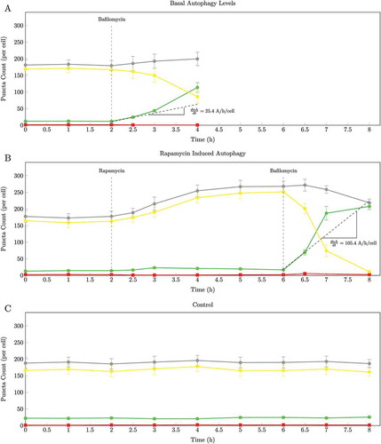
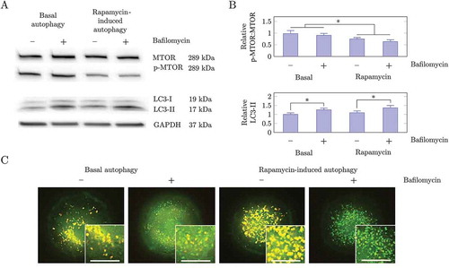
Figure 4. Methods used to assess autophagic activity. (a) Western blot analysis of MTOR, p-MTOR and LC3A/B-II under basal and rapamycin-induced conditions in the presence and absence of the fusion inhibitor BAF. Treatment with 25 nM rapamycin decreased the level of phosphorylation of MTOR, indicating that MTOR was inhibited by rapamycin. Treatment with 25 nM rapamycin caused a greater relative increase in LC3A/B-II after 2 h BAF treatment as compared to basal conditions, indicating that autophagic flux had increased by factor of 2.15. (b) Quantification of western blot analysis of the ratio of p-MTOR:MTOR and LC3A/B-II relative to basal conditions. (C) Fluorescence microscopy analysis of MEF GFP-LC3B cells with 75 nM LysoTracker Red. Cells treated with 25 nM rapamycin showed a small increase in the number of autophagosomes whereas autolysosomes increased significantly. Following BAF treatment there was an increase in autophagosomes and a decrease in autolysosomes. Fluorescence micrographs were acquired in multiple z-planes to quantify the complete autophagosome, autolysosome and lysosome pool size. Images shown here are projections of the z-stack images. Scale bar: 20 µm.

Autophagic variables

The method above describes how to measure the autophagosome flux (Jbasal or Jinduced) as well as the autophagic entities (nA, nAL and nL). In addition to autophagosome flux, other autophagic variables can be derived that are of importance and that characterize the cellular system. One such variable is the transition time, τ, i.e., the ratio of n/J; τ indicates the turnover time of the respective pool at steady state, in other words the time required for the cell to clear the pool of the autophagic vesicles in question. Another useful variable is the cytoplasmic volume consumption rate, Jvol, which describes the relationship between autophagosome flux and autophagosome volume at steady state. This is important, because both autophagosome size and autophagosome flux contribute to the total cargo turnover. The autophagosome and autolysosome volume can be calculated using the radius of the puncta of the respective autophagic vesicles based on the assumption that they are all spherical in nature. The table below summarizes the functional variables of basal and rapamycin-induced autophagy that have been measured for MEF cells through the method described above.

Notes

1. Fluorescent tags. Here we describe a protocol using the MEF cell line that stably expresses GFP-LC3B, which allows the visualization of autophagosomes as green puncta, over time in a single cell. The fusion of autophagosomes with lysosomes results in the formation of autolysosomes that contain lumenal GFP-LC3-II, which is then degraded alongside the autophagic cargo. GFP-LC3-II residing on the outer membrane of the autolysosomes is cleaved from the vesicle and recycled [1]. The acidic lumen of autolysosomes results in the denaturation of GFP and the subsequent loss in fluorescent signal. We observed that GFP signal is not immediately quenched upon fusion of autophagosomes and lysosomes. Therefore, GFP may be regarded as an autophagosome marker, with its absence or its quenching indicating beginning degradation of cargo. LysoTracker Red, an acidotrophic fluorescent marker, allows for the identification of lysosomes, and more importantly, the colocalisation with the GFP fluorescent signal identifying autolysosomes (Figure 1(b)). Once the autophagic cargo is degraded, amino acids are released into the cytoplasm and the autolysosome is recycled contributing to the lysosome pool.

It is important to note that even minor deviations in LysoTracker Red concentrations can affect the fluorescence signal adversely. We observed that concentrations below 75 nM resulted in the rapid dissipation of the fluorescence following BAF treatment, because it results in the de-acidification of lysosomes and autolysosomes, and the concomitant dispersal of the fluorescent dye. At 75 nM, however, the concentration of the fluorescent probe is high enough (and well tolerated) that following BAF treatment the fluorescent emission signal remains sufficient in the vesicle after 1 h of BAF to quantify autolysosomes and lysosomes and to determine the autophagosome flux accurately. Similar results are achieved when using lysosomal membrane tags, such as RFP-LAMP1, in the place of LysoTracker Red probe (Fig. S5). Because the initial slope of the progress curve is the most accurate representation of the autophagosome flux, the short exposure to BAF is sufficient to allow pool size quantification before the signal dissipates. There are many alternative fluorescence tags and dyes commercially available that can be used to distinguish between autophagosomes and autolysosomes. One such fluorescent tag is the tandem GFP-mCherry-LC3 construct, which, depending on the lumenal pH of the vesicle micro-environment, will emit a fluorescence signal either in yellow, indicating autophagosomes, or red, indicating autolysosomes and lysosomes (because autolysosomes are recycled to lysosomes). Fig. S5 shows the autophagosome flux analysis using 2 separate constructs, GFP-LC3B and RFP-LAMP1, to assess autophagosomes, autolysosomes and lysosomes as green, yellow (the colocalization of the green and the red) and red puncta.

1. Slides. In order to improve the statistical power and to compensate for intercellular morphological effects over long periods of time, especially when working with actively proliferating cells such as MEFs, we recommend using FN1 (fibronectin 1) micropatterned slides to temporarily immobilize the cell and to enhance data accuracy. This approach will allow for better control of cell shape, thereby reducing variability, while allowing each cell to be treated as an experimental unit.

2. Software and microscopy. Our protocol to measure autophagosome flux relies on the accurate assessment of autophagosomes and autolysosomes in a single cell over time. Processing image stacks prior to analysis in order to maximally enhance fluorescence signal and minimize background noise improves the accuracy of the autophagosome and autolysosome count.

We used the Olympus IX81 Cell R imaging software to deconvolute image stacks in 3D to enhance the fluorescence signal and improve the puncta analysis. The image brightness and contrast was adjusted to further improve signal/background ratio – although in most cases deconvolution alone was sufficient. Images acquired via laser scanning microscopy techniques would not require deconvolution because the confocality reduces out of focus signal. However, we found that confocal image acquisition takes considerably more time compared to a widefield-based acquisition, which in turn affects accuracy, in particular when vesicular movement impacts on the colocalization signal. Counting of green (autophagosome), yellow (autolysosome) and red (lysosome) puncta can be done in 2D (with a maximum z projection) or in 3D. Automated counting software, such as WatershedCounting3D [9], which is an open source automated counting plug-in for ImageJ [10], can be used to count puncta rapidly and objectively in 3D. We made use of a modified version of WatershedCounting3D that allowed us to analyze multiple images in a high-throughput manner with results being exported as a text file, which was then further processed using Python programming to obtain average and standard deviation of the number puncta per analyzed time point. There are various commercially available software solutions that may be used to count puncta as well as open source counting software such as the ImageJ “particle count/analysis” function. One can also use a manual “touch count” function by manually mouse clicking on the puncta of interest using a projected image stack. The ability to detect the number of autophagosomes, autolysosomes and lysosomes can vary depending on the software used to analyze images that could potentially result variation in data.

1. Quantification of the complete autophagosomal and autolysosomal pool size. In order to accurately quantify autophagosome flux, a precise measurement of the complete intracellular autophagosome and autolysosome pool size is required. It is important when setting up the acquisition protocol that the acquisition time is minimized to avoid autophagosome movement during the acquisition process. One can also improve the autophagosome, autolysosome and lysosome count by making use of higher numerical aperture objectives. Here, the signal/noise ratio of fluorescence signal is further improved, with subsequent deconvolving of images and by adjusting color thresholds. The automated counting software can then be used to rapidly and objectively count puncta via an open source ImageJ plug-in based on a modified Watershed algorithm. The search parameter for the image-based analysis requires optimization.

1. Verifying steady state. This is a crucial step in the process of measuring the autophagosome flux. When the number of autophagosomes per cell stays constant over time, the system is in a steady state. The establishment of a steady state can potentially take a long period of time. For instance, when using drugs that influence the degree of acetylation that can affect autophagic activity, we recommend 2 strategies: (i) to increase the intervals at which the autophagosomal pool size is measured (e.g., every 3 h), or (ii) to measure nA with an hourly interval (3 time points) and, if the autophagic system is not at steady state, to leave the cells for a further 12 h and then assess whether a steady state has established. There are various factors besides stochasticity that should be taken into account when determining steady state. Autophagy is modulated by nutrient availability, energy status and cell density, all of which can affect the autophagosome flux; these factors must therefore be carefully controlled, especially over prolonged periods of image acquisition.

2. Complete inhibition of autophagosome and lysosome fusion. The goal is to determine the concentration of a fusion inhibitor required to completely inhibit the fusion between autophagosomes and lysosomes prior to the execution of the flux experiment. We used BAF; alternatively any vacuolar-type H+-ATPase such as leupeptin or chloroquine may likely be used. Note that following the treatment with a fusion inhibitor it is better to use small time intervals for measurements because it will more accurately reflect the initial slope of the progress curve, and hence the autophagosome flux. It is crucial to determine the concentration of fusion inhibitors required to completely block the fusion between autophagosomes and lysosomes, because a residual flux can persist through the system which may mask the real flux. Furthermore, it is important to establish the necessary concentration required for complete fusion inhibition for each cell type and fusion inhibitor.

3. Measuring autophagosome flux. The autophagosome flux, J, is the initial slope of the progress curve at the point of inhibition of fusion. The initial increase in autophagosome number following inhibition should be carefully monitored for at least 2 h in small time intervals. The smaller the time interval, the more accurate the autophagosome flux can be calculated. We recommend however not to use too small-time intervals, because excessive exposure to high intensity light/laser during image acquisition can lead to phototoxicity. When calculating the autophagosome flux from the slope do not use large time points such as hours postinhibition as they would lead to an unreliable flux due to other factors such as feedback mechanisms.

4. Reliability of data. Various steps can be taken to ensure high reliability and robustness of the data. The first step is monitoring the sum of the green and yellow puncta following the BAF treatment (the gray lines in Figures 2 and 3). In theory the sum of the green and yellow puncta should remain constant following BAF treatment (for a brief period) because the rate of autophagosome synthesis is equal to the rate of autolysosome degradation. This is characterised by an autophagosome pool size that increases at the same rate as the autolysosome pool decreases, the sum of the 2 pools remaining constant. This scenario would only be stable for a few minutes after inhibition. Comparing the sum of the 2 before and after the inhibition at steady state allows one to check the reliability of the count. A significant difference would suggest that there is a residual flux masking the true autophagosome flux. The second step is to monitor in parallel a control condition over time without the presence of any inducers and inhibitors; this serves as a control for potential external factors that may influence the data. A constant number of autophagosomes (nA) over time would indicate a stable control condition (Figure 3(c)) Additionally, knockdown or knockout models can be used as a negative control. Here, a transient ATG5 knockdown model was used (Fig. S6). ATG5 together with ATG12 forms the ATG12–ATG5 complex, which conjugates with ATG16L1 to form a multimeric complex playing an essential role in autophagosome formation. The ATG12–ATG5-ATG16L1 complex participates in the lipidation process of LC3 to form LC3-II, and acts as a scaffolding protein during autophagosome formation [1]. The reduction of ATG5 protein levels thereby limits autophagosome formation.

5. Statistics and Practical Considerations. Autophagy activity can vary significantly between cell types, but also within a cell population. The variation in autophagic activity can arise from several factors such as cell cycle, nutrient availability, phototoxicity, local pH or ionic strength. Hence, a high degree of technical control is required to control for a stable microenvironment. The above mentioned notes describe several steps that can be taken to reduce inter-cellular variably and to enhance technical control of the microenvironment. Micro-patterning, as employed here, can be a valuable tool to standardize cells as an experimental unit through controlling their shape and mobility. Furthermore, performing autophagosome flux analysis on cells that are synchronized, will further decrease intercell variability. In particular, when micropatterning is coupled to modified high-throughput image acquisition [11], variation will be minimized tremendously and statistical power maximized. It will however be crucial to perform z-stack image acquisition with a high NA objective, in order to capture the complete autophagosome pool. Such optics are usually available as water immersion objectives in high-throughput imaging systems. Moreover, we suggest using a large number of cells for statistical analysis. The sample size required depends on the cell type and the inherently observed variability. This protocol is highly applicable, especially for cell types that adhere well, so ensuring optimal morphometric analysis, and can also be implemented using primary isolated cells from, for example, transgenic GFP-LC3 model systems such as mice [12], zebrafish [13], Drosophila [14] or C. elegans [15]. If prepatterned commercially available dishes are utilized instead of self-fabricated masks and culture plates, significant time can be saved, and flux data generated within approximately 8 h. Moreover, when using these for acquisition in a high-throughput imaging platform, technical skills required can further be reduced, due to the degree of automation and autofocus functionalities. The autophagosome flux of individual cells can be used for statistical analysis of a treatment group; mean, standard deviation and standard error of the mean, as well as one-way ANOVA analysis with Bonferroni post-test can be used to determine significant changes in autophagosome flux between treatment groups.

5. Discussion

Measuring autophagic activity

The accurate assessment of the autophagic flux has been a challenge. We have previously proposed the approach of metabolic control analysis to study autophagy [8], but there was still a need for a standardized tool for measuring autophagosome flux and the pool sizes of autophagosomes, autolysosomes and lysosomes. Here we describe a protocol for measuring these autophagic variables (J, nA, nAL and nL) and their derivatives (τA, τAL, Jvol and Jmem).

Western blot analysis is commonly used to assess autophagosome turnover by measuring LC3-II abundance before and after inhibiting the fusion of autophagosomes and lysosomes [16]. From the relative increase in LC3-II abundance, one can infer whether autophagic flux has increased, decreased or remained unchanged. Figure 4(a) illustrates how western blot analysis is used to assess autophagic flux. Although this method is a powerful technique to assess autophagic activity, it is not highly sensitive and also does not measure flux as a rate of flow through the whole pathway (Fig. S4).

Microscopy techniques can directly measure the number of autophagosomes in cells and tissues. TEM is considered the gold standard in many autophagy research applications due to its ability to produce high-resolution images for the identification and morphological analysis of autophagic vesicles. However, unless TEM tomography or serial block-face EM is performed to capture an entire cell volume, EM yields only a partial vesicle pool size, which renders this method more suitable for high-resolution morphological assessments. Measuring the autophagosome flux requires the dynamic assessment of the entire autophagosome pool over time, making TEM unsuitable because it does not allow for time-lapse analysis. In fact, TEM analysis of a similar sample resulted in less accurate data, compared to fluorescence microscopy derived results (Fig. S4).

The protocol described here demonstrates that fluorescence microscopy allows whole cells to be optically sectioned, so that complete pools sizes can be measured. It allows LC3-positive structures in living cells and tissues to be visualized over time [17,18]. Measuring the autophagosome flux in fact requires the dynamic assessment of autophagosomes over time in the presence and absence of a fusion inhibitor. Although fluorescence-based methods have been used to assess whether or not autophagic activity is occurring, e.g., by using a mCherry-LC3 transgenic mouse model and by measuring the surface area of the fluorescence signal before and after administration of fusion inhibitors [6], the calculation of flux requires the numerical quantification of the autophagic vesicles over time.

Recent advances in live cell imaging confirm the power of fluorescence imaging in assessing autophagy activity [19], but to date they have not been used to assess autophagic variables (J, nA, nAL and nL) and their derivatives (τA, τAL, Jvol and Jmem) under basal or induced conditions in different cell types. Nevertheless, they have led to the development of novel techniques that can indirectly assess autophagic degradation based on the rate of decay of cytosolic proteins. One such method uses cytosolic photo-activatable fluorescent proteins that, once activated, can be used to measure the rate of decay of the fluorescence signal in the cytoplasm, which gives an indication of the rate of protein degradation in general [7]. Although this approach does measure a rate, it provides little data on the autophagosome pool size and its rate of change over time. A recent study measured the number of GFP-LC3-II-positive autophagic vesicles per cell over time in the presence and absence of a fusion inhibitor [20]. Similar to the approach presented here, the reasoning was that one can determine the rate of autophagosome synthesis from the initial rate of accumulation in autophagosomes following the complete inhibition of the fusion of autophagosomes and lysosomes. However, in this study GFP-LC3-II-positive autophagic vesicles were equated to autophagosomes, which likely results in inaccurate flux measurements because they include autolysosomes. Moreover, the crucial step of verifying complete fusion inhibition and assessing whether cells were indeed in steady state before treatment with fusion inhibitor was absent.

Autophagic variables

Our conception of the autophagic pathway as a multi-step pathway along which there is a flow of material that is similar to that of a metabolic pathway, which consists of a series of steps linked by a common intermediate, each step characterized by its own rate. The variable entities that participate in the autophagic pathway are the autophagosomes (nA), autolysosomes (nAL) and lysosomes (nL). The autophagosome flux J is the rate of flow along the vesicular pathway at steady state. Our method allows the characterization of autophagy steady states in terms of (i) a complete nA, nAL and nL, (ii) autophagosome flux J, (iii) the transition times τA and τAL, (iv) cytoplasmic volume consumption rate, Jvol, and (v) autophagosomal membrane flux Jmem (Table 1). Note that the transition time of lysosomes is not calculated using the autophagosome flux because lysosomal turnover is not dependent on the autophagosome flux, as it is transcriptionally regulated [21]. The transition time, τ, and the cytoplasmic volume consumption rate, Jvol, are potentially useful when assessing cells with either increased or dysfunctional autophagosome clearance.

Table 1. Functional variables of autophagy as measured by the here presented protocol.

Variable	Unit	Basal	Induced
Autophagosome flux, J	A/h/cell	25.4	105.4
Number of autophagosomes, nA	A/cell	13.4	16.7
Number of autolysosomes, nAL	AL/cell	164.5	251.2
Average volume of an autophagosome	fL	4.3	4.7
Average volume of an autolysosome	fL	17.3	18.8
Autophagosomal transition time, τA	h	0.53	0.16
Autolysosomal transition time, τAL	h	6.7	2.4
Cytoplasmic volume consumption rate, Jvol	fL/h/cell	109	495
Autophagosomal membrane flux, Jmem	µm2/h/cell	1397	8268

A, autophagosomes; AL, autolysosomes. Derived variables are shown in italics.

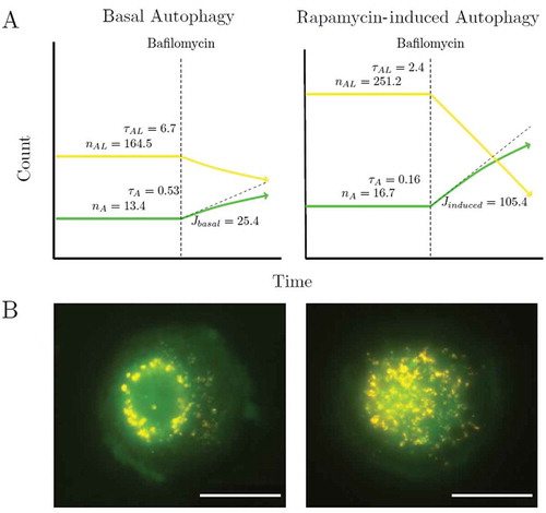
Figure 5 shows the characterization of basal and rapamycin autophagy variables. The autophagic variables can be used for evaluating the response of the autophagic system to pharmacological regulators, by quantifying the difference between the steady states of the treated and untreated cells in terms of their changes in autophagosome and autolysosome pool size (∆nA and ∆nAL), autophagosome flux (∆J) and transition time upon intervention (∆τA and ∆τAL). Hence, this protocol may be highly suitable to complement current approaches in the context of autophagy drug discovery or library screening. Here, the protocol may be amended to include concentration ranges in order to dissect their impact on pool size, autophagosome flux and transition time. Such an approach would be particularly useful to assess upstream autophagy modulators whereas drugs that de-acidify lysosomes are less suitable to be assessed in this manner.

Figure 5. Basal and rapamycin-induced autophagy variables. (a) A cartoon shows a cartoon of basal and induced autophagy variables. (b) Representative images of basal and rapamycin-induced steady state autophagy. J = autophagosomes/h/cell, ni = number of steady-state species and τi = h.

Limitations

The protocol described makes use of live cell imaging to monitor the formation and degradation of the autophagic intermediates. This method is well suited to analyze the autophagosome flux and pathway intermediates and can derive several useful variables of the autophagic system. However, the method as described here, focusing on vesicle dynamics, is less suited for measuring other aspects of the autophagic system, such as specific or general cargo degradation. This protocol rather provides a complimentary tool to assess and finely dissect to what extent different autophagy inducing drug concentrations impact autophagosome flux, but it would reflect little on the regulatory pathway itself. Finally, this protocol lacks optical resolving power and provision of ultrastructural detail. Moreover, this method is entirely based on the use of light microscopy and fluorescent probes, which inherently introduces technique-associated challenges such as photo-bleaching, photo-toxicity and various sources of noise, all of which may impact on the signal/noise ratio.

Concluding remarks

This protocol describes a unique approach to measuring the autophagosome flux by assessing the complete autophagosome pool size over time and its increase following the inhibition of fusion with BAF. This approach differs from currently established fluorescence-based methods in that it is used to calculate the autophagosome flux from the initial rate of increase (autophagosomes/cell/h) in autophagosomes after inhibition with BAF. This approach provides a robust and sensitive tool for measuring autophagosome flux, which can be used to (i) characterize autophagic steady states and autophagosome flux in key cell and tissue types of clinical relevance, (ii) characterize cell and tissue types of key disease states and deviations in autophagosome flux, and (iii) scoring pharmacological regulators of autophagy to enable the generation of data that allow a better alignment between autophagy-modulating drugs and deviations of flux observed in disease states, so as to re-establish physiological autophagy flux and proteostasis.

Acknowledgments

We wish to thank Noboru Mizushima, University of Tokyo, for providing the GFP-LC3 MEF cells.

Disclosure statement

B.L., J.H.S.H. and A.dT. are inventors on a patent entitled 'Method of determining autophagosome flux and uses thereof' (PCT/IB2017/052732). The remaining author, T.J.G. declares no competing interest.

Supplementary material

Supplementary data for this article can be accessed here.

Additional information

Funding

The authors acknowledge financial support from the South African National Research Foundation (NRF), the South African Medical Research Council (SAMRC) and the Cancer Association South Africa (CANSA). Any opinion, findings, and conclusions or recommendations expressed in this material are those of the authors, and therefore the NRF, SAMRC and CANSA do not accept any liability in regard thereto. National Research Foundation South Africa; South African Medical Research Council (MRC).

References

- Levine B, Klionsky DJ. Development by self-digestion: molecular mechanisms and biological functions of autophagy. Dev Cell. 2004;6(4):463–477.
- Choi AM, Ryter SW, Levine B. Autophagy in human health and disease. N Engl J Med. 2013;368(7):651–662.
- Klionsky DJ, Abdalla FC, Abeliovich H, et al. Guidelines for the use and interpretation of assays for monitoring autophagy. Autophagy. 2012;8(4):445–544.
- Haspel J, Shaik RS, Ifedigbo E, et al. Characterization of macroautophagic flux in vivo using a leupeptin-based assay. Au- Tophagy. 2011;7(6):629–642.
- Tooze SA, Yoshimori T. The origin of the autophagosomal membrane. Nat Cell Biol. 2010;12(9):831–835.
- Iwai-Kanai E, Yuan H, Huang C, et al. A method to measure cardiac autophagic flux in vivo. Autophagy. 2008;4(3):322–329.
- Tsvetkov AS, Arrasate M, Barmada S, et al. Proteostasis of polyglutamine varies among neurons and predicts neu- rodegeneration. Nat Chem Biol. 2013;9(9):586–592.
- Loos B, du Toit A, Hofmeyr JHS. Defining and measuring autophagosome flux– concept and reality. Autophagy. 2014;10(11):2087–2096.
- Gniadek TJ, Warren G. WatershedCounting3D: A new method for segmenting and counting punctate structures from confocal image data. Traffic. 2007;8(4):339–346.
- Abr`Amoff MD, Magalh˜aes PJ, Ram SJ. Image processing with ImageJ. Biophoton Int. 2004;11(7):36–43.
- Zhang L, Yu J, Pan H, et al. Small molecule regulators of autophagy identified by an image-based high-throughput screen. Proc Natl Acad Sci USA. 2007;104(48):19023–19028.
- Mizushima N, Yamamoto A, Matsui M, et al. In vivo analysis of autophagy in response to nutrient starvation using transgenic mice expressing a fluorescent autophagosome marker. Mol Biol Cell. 2003;15(3):1101–1111.
- He C, Klionsky DJ. Analyzing autophagy in zebrafish. Autophagy. 2010;6(5):642–644. PMID: 20495344.
- Berry DL, Baehrecke EH. Growth arrest and autophagy are required for salivary gland cell degradation in Drosophila. Cell. 2007;131(6):1137–1148.
- Chang JT, Kumsta C, Hellman AB, et al. Spatiotemporal regulation of autophagy during Caenorhabditis elegans aging. eLife. 2007;6:e18459.
- Rubinsztein DC, Cuervo AM, Ravikumar B, et al. In search of an ”autophagomometer”. Autophagy. 2009;5(5):585–589.
- Ni HM, Bockus A, Wozniak AL, et al. Dissecting the dynamic turnover of GFP-LC3 in the autolysosome. Autophagy. 2011;7(2):188–204.
- Bampton ETW, Goemans CG, Niranjan D, et al. The dynamics of autophagy visualized in live cells: from autophagosome formation to fusion with endo/lysosomes. Autophagy. 2005;1(1):23–36.
- Kaizuka T, Morishita H, Hama Y, et al. An autophagic flux probe that releases an internal control. Mol Cell. 2016;17(64):835–849.
- Martin KR, Barua D, Kauffman AL, et al. Computational model for autophagic vesicle dynamics in single cells. Autophagy. 2013;9(1):74–92.
- Sardiello M, Palmieri M, di Ronza A, et al. A gene network regulating lysosomal biogenesis and function. Science. 2009;325(5939):473–477.