Parametric CAPEX, OPEX, and LCOE expressions for offshore wind farms based on global deployment parameters

ABSTRACT

Installed wind energy capacity has been rapidly increasing over the last decade, with deployments in deeper waters and further offshore, with higher turbine ratings within new farms. Understanding the impact of different deployment factors on the overall cost of wind farms is pertinent toward benchmarking the potential of different investment decision alternatives. In this article, a set of parametric expressions for capital expenditure, operational expenditure, and levelized cost of energy are developed as a function of wind turbine capacity (), water depth (WD), distance from port (D), and wind farm capacity (). These expressions have been developed through a series of simulations based on a fully integrated, tested cost model which are then generalized through the application of appropriate nonlinear regression equations for a typical offshore wind farm investment and taking into account most current published cost figures. The effectiveness of the models are countersigned through a series of cases, estimating the predicted values with a maximum error of 3.3%. These expressions will be particularly useful for the preliminary assessment of available deployment sites, offering cost estimates based on global decision variables.

KEYWORDS:

• CAPEX
• LCOE
• nonlinear regression
• offshore wind farm
• OPEX
• parametric expressions

Introduction

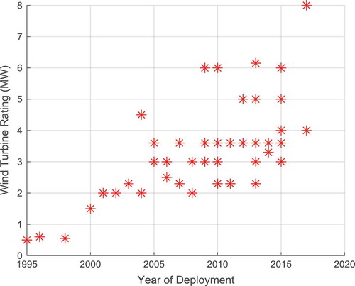
Latest targets for Europe as reported from Wind Europe aim for 320 GW of wind energy capacity to be installed by 2030, 66 GW of which is planned to come from offshore wind (OW) energy (EWEA 2015). Deployment in deeper waters and further offshore is driven by the higher wind speeds, unrestricted space, and lower social impact in the marine environment (Kolios et al. 2016; Regueiro-Ferreira and Villasante 2016), where it is estimated that the same wind turbine can produce around 50% higher power output compared to onshore. High construction costs, especially foundation and electrical connection, and limitations in operation and maintenance are key barriers that need to be overcome in order to deploy in such environments in a cost-effective way. Figure 1 presents processed data from commissioned wind farms with respect to deployment depth, distance from shore, and wind farm capacity, while Figure 2 shows the increase in installed wind turbine ratings from 1995 to 2017 based on data from 4C Offshore 2017.

Figure 1. Water depth vs. distance to shore vs. wind farm capacity.

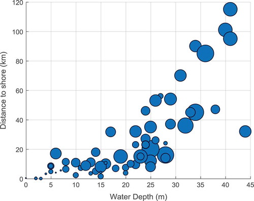
Figure 2. Turbine rating vs. wind farm year of commissioning.

Reference to cost figures across the life cycle of existing wind farms has been limited to date with high volatility of cost components, primarily due to the fact that the industry and its supply chain have not yet been fully developed. Understanding, however, the impact of different deployment factors to the overall cost of wind farms becomes pertinent toward benchmarking the potential of different investment decision alternatives.

This article reports the development of a set of parametric models for capital expenditure (CAPEX), operational expenditure (OPEX), and levelized cost of energy (LCOE) as a function of a set of global variables for potential deployment sites. These account for the wind turbine capacity (), water depth (WD), distance from port (D), and wind farm capacity (). These variables were selected due to their significant effect on the cost-effectiveness of the investment (Shafiee et al. 2016). After mapping the multidimensional cost domain based on these variables, through a series of simulations performed by a fully integrated and tested cost model developed by the author, results are translated into analytical expressions to interpolate cost figures for potential wind farms within the applicability range of the expressions. A parametric analysis and a number of test cases illustrate the effectiveness of the models, drawing useful conclusions.

These expressions are expected to assist investors, researchers, and other stakeholders to undertake an initial estimate of CAPEX, OPEX, and LCOE values for OW farm projects with varying design parameters, as well as use them as reference for estimating the effect in the change of one of the selected design parameters. The cost model developed incorporates the most up-to-date available parametric expressions in the literature, while where such equations were not available, most recent data were gathered in order to model specific costs.

Cost model of OW farm with fixed monopile

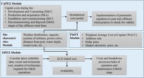
The main components of the life-cycle cost of a fixed OW farm are distinguished and further decomposed to cost subcomponents as shown in Figure 3, while in Figure 4, the cost model framework that has been developed is presented. Throughout the model, the most up-to-date expressions for cost subcomponents have been employed. The life-cycle phases under which costs were categorized are as follows: design and consent (C₁), production and acquisition (C₂), installation and commission (C₃), operation and maintenance (C₄), and decommissioning and disposal (C₅), a categorization scheme adopted by numerous recent studies (Myhr et al. 2014; Shafiee et al. 2016; The Crown Estate 2010). Total life-cycle cost is, thus, defined as

(1)

Figure 3. Breakdown of life-cycle costs.

Figure 4. Integrated cost model structure.

The design and consent costs were further decomposed to legal (), environmental survey (), engineering (), contingency (), and project management () costs. The costs of this stage were considered to be proportional to the wind turbine capacity () according to Shafiee et al. 2016, although other parameters such as the water depth and marine life in the installation location can also affect the cost because of the lack of data.

The production and acquisition stage can be further decomposed to the following: the acquisition of the turbine (), the foundation (), the electric system (), and the control system (). The cost of the turbine was estimated as a function of the wind turbine capacity (, while the cost of foundation as a function of the , , h, and d (; Dicorato et al. 2011).

The cost of the electric system comprises the cost of array, export and onshore cables (), and the cost of the substation (); the first, depending on the number of the wind turbines (), the rotor diameter (d), and the distance from shore (D)—; the second, depending on the number of the wind turbines, rated power of transformer (), the nominal voltage transformer (), and the wind farm capacity () according to Dicorato et al. 2011—. Onshore substation cost was assumed to be half the cost of the offshore substation. The control system cost was also taken from the same source to be equal to  = 75 k£/turbine.

Next, the installation and commissioning costs of the OW farm comprise the installation of the wind turbine and tower (), foundation and transition piece (), scour protection (), electric system (), and the insurance costs (), a categorization also used by BVGA 2010, Dicorato et al. 2011, and Shafiee et al. 2016. The installation cost of the wind turbines is a function of the vessel day rates (), the number of vessels (workboats, heavy lift vessels, Special Operations Vessels (SOVs), and jack up vessels; ), the duration of the installation (), and the cost for the personnel () required for carrying out the installation. Specifically for the installation of the wind turbines, the onshore pre-assembly method () is also expected to greatly affect the cost of installation (Sarker and Faiz 2017). Although installation usually takes place during spring and summer time in order to avoid adverse weather conditions, they still play an important role to activities taking place offshore (Kaiser 2009); hence, for estimating the final installation cost of the wind farm, a weather adjustment factor () was also considered, an approach used also by other authors in the literature (Sarker and Faiz 2017; Kaiser and Snyder 2012). Therefore, the cost is expressed as . Roughly, the installation of all components of the wind farm depends on similar factors; nevertheless, vessels with different load capacity and different procedures are followed for the installation of each component.

The operation and maintenance stage of the life cycle is further decomposed into the repair (), the rent (), the insurance (), and the project management cost (). The estimation of the repair cost was carried out through the Energy Research Centre of the Netherlands Operation and Maintenance (ECN O&M) tool (Van De Pieterman et al. 2011), which divides O&M strategies into calendar-based, condition-based, and unplanned corrective operations. For unplanned corrective maintenance, each structural component of the system is assigned a number of failure modes bearing different severity and frequency levels, which is introduced in the software by means of a mean time to failure. The different fault type classes are classified as minor repairs, major repairs, and major replacements following the Reliawind categorization scheme (Wilkinson et al. 2010). Further data needed for the prediction of the unplanned corrective maintenance costs include the average repair times, number of required technicians, and material costs, which were adopted from Carroll et al. 2016. For the condition-based maintenance, a certain number of repairs can be set for inclusion, while the calendar-based maintenance applies to all turbines of the wind farm. For calendar-based maintenance, a yearly small maintenance operation and a longer one occurring every 5 years were considered.

Decommissioning and disposal cost of the wind farm includes the following: the removal of the wind turbine (nacelle, tower, and transition piece) as well as the balance of the plant (foundations, scour protection, cables, and substations; ), the site clearance (), the onshore transportation to the disposal sites (), the port preparation (), the disposal process (), and finally the hiring vessels costs (). To accomplish this stage of the life cycle, jack-up vessels are used to transport the removed items to shore, as well as workboats to transfer personnel who will support the operation. Substations are also removed by means of a reverse installation process (with the support of a heavy lift vessel), and the jacket foundations are also cut and removed. Removal costs depend on the removal duration per turbine (), the capacity of the jack-up vessel (), the vessels’ day rate (), the number of vessels (workboats, heavy lift vessels, SOVs, and jack-up vessels) (), and the cost of technicians (). As such, . The site clearance cost depends mainly on the area of the wind farm, which can be calculated by taking into account the rotor diameter and the number of wind turbines, as well as a mean clearance cost per km² (), as in (Kaiser and Snyder 2012) . The transportation cost is associated to the total mass of the wind farm components (), the truck cost per ton-mile (), the capacity of truck (), and the distance of port from the waste facility (): .

Case study presentation and application

Key assumptions of the wind farm site under the baseline scenario are included in Table 1. The 504 MW wind farm is located in the North Sea region. For the calculation of the energy produced under the baseline scenario, the availability factor derived from analysis through the O&M simulation was used (calculated 91.2%). Further, an efficiency factor of 90% was assumed accounting for losses due to wake effects, cable losses, and so on. The electrical system consists of 33 kV array cables and two offshore substations of 336 MW HVAC transmission system. Additionally, the transmission assets are connected to the onshore substation by three AC export cables of 132 kV.

Table 1. Baseline specifications.

Characteristic values of the 3.6 MW wind turbine used for the baseline scenario
Total wind farm capacity,	504 MW
Nameplate capacity,	3.6 MW
Distance to port, D	36 km
Water depth, WD	26 m
Service life of the wind farm	25 years
Rotor diameter	107 m
Hub height	77.5 m
Pile diameter	6 m
Rated wind speed	13.5 m/s
Cut-in wind speed	4 m/s
Cut-out wind speed	25 m/s

The total undiscounted CAPEX aggregating,,, and were estimated equal to 1,698.3 M£, while the mean undiscounted annual OPEX was found around 56.3 M£/year under the baseline scenario. Nevertheless, the above figures need to be adjusted for the inflation rate and the interest rate, in order to account for the time value of money considering that the service life of an OW farm is approximately 25 years. All costs were therefore discounted and inflated with the real discount rate () integrating the nominal cost of capital () with the inflation rate (), according to Fisher equation (Barro 1997)

(2)

where was assumed equal to 8.81% (BVGA 2015) and 2.5%. Further, the levelized cost of energy (), which estimates the net present value of the unit cost of electricity produced over the lifetime of the OW asset, can be calculated as

(3)

where (£) is the life time duration of the wind farm (from construction to decommissioning) and E (MWh) is the total energy produced. Taking the above into consideration, the baseline LCOE was estimated 112.6 £/MWh, the discounted total OPEX () 559 M£, and the discounted CAPEX () 1,351.9 M£. The above results conform well with the literature levelized cost estimates for Round 3 OW projects commissioned in 2020 (BEIS 2016). Finally, the resulting capacity factor was calculated (38.8%).

The parametric relationships linking the four key design parameters—namely, the wind turbine capacity, water depth, distance from port, and wind farm capacity with the OPEX, CAPEX and LCOE figures—were derived through nonlinear regression from a number of simulations of the integrated cost model aiming to map the cost performance across the multidimensional domain of the four independent variables. A set of complex relationships was assumed for this study based on the observation of the relationship between the input global parameters and the output variables (dCAPEX, dOPEX, and LCOE), ensuring a realistic approximation and avoiding cases of overfitting which may reduce accuracy in the results. The outcome of the finite number of scenarios that were run in order to map the cost domain is listed in Table 2, where the effect of the variable variation on CAPEX, OPEX, and LCOE can also be observed. It was shown that wind turbine and wind farm capacity have the greatest effect on CAPEX, OPEX, and LCOE. In fact, doubling the while keeping the rest of the variables stable results in 14%, 5.2%, and 5.8% decrease in the respective investment performance indicators; the corresponding effect of resulted in 77%, 92.3%, and −2.4% variation from the baseline case. The next most impactful variable on LCOE proved to be the distance from port.

Table 2. Results from the application of the model to a number of scenarios.

Scenario	(MW)	(m)	(km)	(MW)	(£)	(£)	LCOE (£/MWh)
Baseline	3.6	26	36	504	559,000,000	1,351,900,000	112.6
#1	1.8	26	36	504	709,750,000	1,512,500,000	135.2
#2	7	26	36	504	481,420,000	1,281,400,000	106.1
#3	5.3	26	36	504	510,370,000	1,274,100,000	110.3
#4	3.6	13	36	504	559,000,000	1,318,500,000	110.7
#5	3.6	52	36	504	559,000,000	1,418,800,000	116.6
#6	3.6	39	36	504	559,000,000	1,385,400,000	114.6
#7	3.6	26	18	504	557,590,000	1,303,500,000	107.6
#8	3.6	26	72	504	573,260,000	1,448,700,000	126.9
#9	3.6	26	54	504	559,390,000	1,400,300,000	115.0
#10	3.6	26	36	252	341,250,000	743,920,000	130.0
#11	3.6	26	36	1008	989,090,000	2,600,300,000	109.9
#12	3.6	26	36	756	771,040,000	1,970,300,000	111.2

Note: Bold numbers indicate which values change (in relation to the baseline case) at each scenario analysed.

Results and discussion

Based on the data presented in Table 1, which illustrate the results of the different scenarios derived from the high fidelity cost model, each of the chosen variables (, , D, and ) was studied independently in order to qualify the most appropriate regression expression to capture the trend in the overall dependent variables. This allowed for a series of nonlinear expressions to be developed, which would better represent these trends not only for interpolation between the limits that were set through the different scenarios but also for extrapolation near these limits. More specifically, it was found from the results of the scenarios that for variable , all three dependent variables were better fitted through power equations. For , OPEX was constant (independent from water depth), while CAPEX and LCOE were better fitted through linear equations. Accordingly, for D, OPEX and LCOE were fitted through exponential and polynomial equations, respectively, while for CAPEX a linear equation was chosen. Finally, for P_WF, linear equations were fitted for CAPEX and OPEX and a power equation for the LCOE.

Once the most appropriate regression expressions were determined, a set of overall relationships were developed for each of the dependent variables, and the nonlinear coefficients were estimated through application of the maximum likelihood method for a predetermined shape of the target equation. The analysis also returned the overall value for the regression coefficients, providing an indication on the overall quality of fit of the quantities considered. Based on the above, the following three expressions are proposed, considering the most up-to-date information and high-fidelity cost modelling structure in order to link the macro variables, namely (MW), WD (m), D (km), and (MW) to the OPEX, CAPEX, and LCOE figures.

(4)

(5)

(6)

The R² for each of the expressions are 0.986, 0.999, and 0.983, respectively, denoting a satisfactory fit to the original data. Further, the data for the independent variables for the different scenarios were used as predictors using the regression coefficients, and the average value of the absolute errors that were measured in each case were 1.62%, 0.83%, and 0.82%. Finally, a series of separate test scenarios were run in order to test the performance of the model while interpolating, and the results are summarized in Table 3.

Table 3. Testing scenarios and results produced by model and parametric expressions.

Testing scenarios		#t1	#t2	#t3	#t4
		6	3.6	3.6	3.6
WD		26	15.6	26	15.6
D		36	36	21.6	21.6
		504	504	504	302.4
(£)	Par. expression	4.872E+08	5.680E+08	5.680E+08	3.984E+08
	Cost model	5.036E+08	5.590E+08	5.569E+08	3.909E+08
	Error (%)	−3.3%	1.6%	2.0%	1.9%
(£)	Par. expression	1.269E+09	1.336E+09	1.324E+09	8.055E+08
	Cost model	1.293E+09	1.325E+09	1.313E+09	8.108E+08
	Error (%)	−1.8%	0.8%	0.8%	−0.7%
(£/MWh)	Par. expression	108.4	110.9	109.3	116.3
	Cost model	107.6	111.1	107.2	115.7
	Error (%)	0.8%	−0.2%	1.9%	0.5%

Note: Bold numbers indicate which values change (in relation to the baseline case) at each scenario analysed.

Following the test scenarios that were run, a series of plots were also produced and are presented in Figure 5, illustrating the effect of each of the independent variables to the dependent ones.

Figure 5. Sensitivity analysis of each parameter: (a) wind turbine rating, (b) distance from port, (c) water depth, and (d) wind farm capacity.

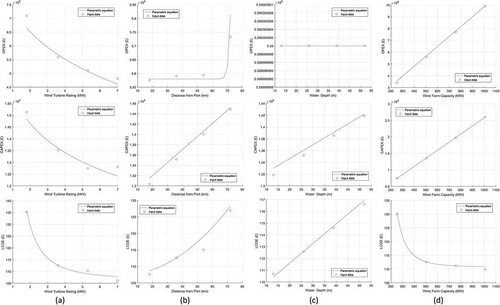
Increase in the wind turbine rating results in an inverse exponential reduction in all three costs: CAPEX and OPEX due to the fact that less units need to be installed and maintained, and LCOE due to the reduced costs and increased expected power production. Distance from shore increases CAPEX linearly, while OPEX and LCOE increase exponentially. Increase in water depth does not affect OPEX, while it results in almost a linear increase in CAPEX and LCOE mainly due to the additional cost of the foundation and support structure as well as installation. Finally, increase in total wind farm capacity increases proportionally the amount of OPEX and CAPEX, while presents an inverse exponential reduction trend to LCOE for the given wind turbine rating due to the higher energy production and the reduced costs per wind turbine. It should be noted that the applicability range of these equations yields mainly for interpolation of values for independent variables, i.e., selection of values within the upper and lower limits included in Table 2. Extrapolating for values significantly out of this range would introduce higher errors as coefficients should be calibrated following a new set of initial simulations with the integrated cost model.

Conclusions

As the OW energy industry is developing, understanding the key cost factors of wind farm developments is a pertinent condition toward benchmarking the suitability of different deployment options. In this work, a set of parametric equations linking wind turbine capacity, water depth, distance from port, and wind farm capacity with the discounted total OPEX, CAPEX, and LCOE figures were developed, based on a number of high-fidelity cost simulations and regressions of the results. Further, this article characterizes the effect of these variables on CAPEX, OPEX, and LCOE. It was shown that wind turbine and wind farm capacity have the greatest effect on CAPEX, OPEX, and LCOE. A future expansion of the model could potentially include more variables, so as to increase the accuracy of results, such as the interest rate which has a considerable effect on LCOE and on the discounted values of capital and operational costs. Further, the inclusion of the wind resource of the installation site could potentially improve the energy output prediction and hence, provide a better informed expression for LCOE; while the inclusion of the soil conditions, aerodynamic, and wind and wave loads at the installation site would increase the accuracy of the production and acquisition cost of the foundations and wind turbines, leading, however, to more complex relationships requiring more input data.

The high-level expressions developed in this work are expected to assist investors, researchers, and other stakeholders to derive initial estimates for wind farm projects based on global variables within the applicability range as defined above. Additionally, it should be highlighted that results from the above expressions should be treated with caution as input data have been adopted from wind farms mainly installed in North Europe, since no data currently exist for the USA or Asian OW farms.

Acknowledgments

This work was supported by grant EP/L016303/1 for Cranfield University and the University of Oxford, Centre for Doctoral Training in Renewable Energy Marine Structures (REMS) (http://www.rems-cdt.ac.uk/) from the UK Engineering and Physical Sciences Research Council (EPSRC).

References

- 4C Offshore. 2017. Global offshore wind farms database. http://www.4coffshore.com/windfarms/.
- Barro, Robert J. (1997), Macroeconomics (5th ed.), Cambridge: The MIT Press, United States of America, ISBN 0-262-02436-5.
- BEIS. 2016. Electricity generation costs. Accessed November, 2016. https://www.gov.uk/government/uploads/system/uploads/attachment_data/file/566567/BEIS_Electricity_Generation_Cost_Report.pdf.
- BVGA. 2010. A guide to an offshore wind farm, BVG associates on behalf of the crown estate. www.thecrownestate.co.uk/guide_to_offshore_windfarm.pdf.
- BVGA. 2015. DECC offshore wind programme – simple levelised cost of energy model. Revision 3–26/10/2015. http://www.demowind.eu/LCOE.xlsx.
- Carroll, J., A. McDonald, and M. David. 2016. Failure rate, repair time and unscheduled O&M cost analysis of offshore wind turbines. Wind Energy 19 (6):1107–19. doi:10.1002/we.1887.
- The Crown Estate. 2010. A guide to an offshore wind farm. London, UK.
- Dicorato, M., G. Forte, M. Pisani, and M. Trovato. 2011. Guidelines for assessment of investment cost for offshore wind generation. Renewable Energy 36 (8):2043–51. doi:10.1016/j.renene.2011.01.003.
- EWEA. 2015. Wind energy scenarios for 2030. Brussels, Belgium: The European Wind Energy Association.
- Kaiser, M. J., and B. F. Snyder. 2012. Offshore wind energy cost modeling – installation and decommissioning. London, UK: Springer-Verlag.
- Kaiser, M. J. 2009. The impact of weather on offshore energy losses. Energy Sources, Part B: Economics, Planning, and Policy 4 (1):59–67. doi:10.1080/15567240701421864.
- Kolios, A., V. Mytilinou, E. Lozano-Minguez, and K. Salonitis. 2016. A comparative study of multiple-criteria decision-making methods under stochastic inputs. Energies 9 (7):566. doi:10.3390/en9070566.
- Myhr, A., C. Bjerkseter, A. Ågotnes, and T. A. Nygaard. 2014. Levelised cost of energy for offshore floating wind turbines in a life cycle perspective. Renewable Energy 66:714–28. doi:10.1016/j.renene.2014.01.017.
- Regueiro-Ferreira, R. M., and S. Villasante. 2016. Recent development of offshore marine power in Galicia. Energy Sources, Part B: Economics, Planning, and Policy 11 (8):760–65. doi:10.1080/15567249.2013.787471.
- Sarker, B. R., and T. I. Faiz. 2017. Minimizing transportation and installation costs for turbines in offshore wind farms. Renewable Energy 101:667–79. doi:10.1016/j.renene.2016.09.014.
- Shafiee, M., F. Brennan, and I. A. Espinosa. 2016. A parametric whole life cost model for offshore wind farms. The International Journal of Life Cycle Assessment 21 (7):961–75. doi:10.1007/s11367-016-1075-z.
- van de Pieterman, R. P., H. Braam, T. S. Obdam, L. W. M. M. Rademakers, and T. J. J. van der Zee. 2011. Optimisation of maintenance strategies for offshore wind farms. The Netherlands: Energy Research Center of the Netherlands.
- Wilkinson, M. et al., 2010. Methodology and Results of the Reliawind Reliability Field Study; European Wind Energy Conference, Warszaw, April 2010.