Gasoline demand in Saudi Arabia: are the price and income elasticities constant?

ABSTRACT

The paper investigates gasoline consumption in case of oil-exporting country applying Time-varying Coefficient Cointegration approach to the data from 1980 to 2017. Empirical estimations show that long-run income and price elasticities are not constant and are responsive to price and income fluctuations in the period considered. The income elasticity of gasoline demand increased until 2014, peaking at 0.151, following growth in disposable income, before declining to 0.136 in 2017. However, consumers do not stop driving when their disposable incomes fall, resulting in a less elastic response of gasoline demand to income. Price elasticities sit in the range of −0.31 to −0.05, becoming less elastic when prices are low and vice versa.

The findings of the study may be useful in successful implementation of energy price reforms and implementation of environmental policies.

KEYWORDS:

• Gasoline demand
• time-varying coefficient
• cointegration
• Saudi Arabia
• elasticity

1. Introduction

After the drop in international oil prices in 2014, oil-exporting countries started to launch new policies to develop their economies. It is important that policymakers involved in energy and economic development understand how economic agents respond to increased energy prices and how the latter affects the demand for different fuels. Saudi Arabia is the biggest oil-exporting country and is currently undergoing many socio-economic reforms. The success of these reforms requires accurate assessments of the country’s energy indicators.

The growth path of gasoline demand, a key strategic fuel, has important implications for oil security, oil-related carbon emissions, and refinery investment (Dahl 2012). As such, understanding how fluctuations in income and gasoline prices could affect the demand for oil in Saudi Arabia allows policymakers to assess what drives gasoline demand over time and the likely future development of oil demand. This knowledge can help demand-side policymakers control oil demand more effectively through the use of measures such as tariffs and taxes, among other instruments. It can also help supply-side decision-makers develop more accurate data on the oil supply needed to meet the anticipated demand and plan refinery investment accordingly. Having a clearer picture of future oil demand could also help the Kingdom to develop the necessary carbon dioxide (CO2) mitigation measures ahead of time, enable government entities to plan transportation services with more certainty, and help car manufacturers project their anticipated sales.

After the fall of global oil prices, many oil-rich countries deployed energy price reforms (EPR) to raise government revenues, while encouraging more rational consumption of energy (see Gonand, Hasanov, and Hunt 2019 for further discussion). The responses of economic agents in oil-exporting countries to changes in the international and domestic economic systems gives useful insights to domestic and international policymakers.

Regional and global stakeholders are currently looking to Saudi Arabia, the biggest exporter of oil, for insights into the possible development paths of their economies. A significant focus is placed on the impact of Saudi Vision 2030 (SV2030), and its various initiatives. For example, the number of female drivers in Saudi Arabia is projected to be around 3 million in 2020 (PwC 2018), following the lifting of the ban on women drivers in the country in 2018 as a part of the SV2030 women’s empowerment policy. This might increase gasoline demand in the near future through direct and indirect channels (such as women driving). PricewaterhouseCoopers (PwC) (2018) also projects car sales will increase by 9% annually up to 2025, against the 3% annual increase between 2013 and 2017.

The analysis presented in this paper is of particular value for Saudi Arabia as it allows policymakers to quantify the impact of SV2030 targets and initiatives, including the possible impacts of price, income, and population on energy demand. These initiatives include the Fiscal Balance Program (FBP), the National Transformation Program (NTP), and the energy price reforms (EPR). The Vision’s goal of energy efficiency, for example, depends on having a clear picture of the numerical impacts of drivers on gasoline demand.

Evidence from data and empirical studies (Algunaibet and Matar 2016, inter alia) show that price elasticity might vary over time.

We use disposable income as an income proxy, which is taken from Mikayilov et al. (2020b), and measured in million SAR at 2010 prices. Looking at the development path of the Saudi economy, the response of gasoline demand to changes in the disposable income level is most likely not constant in the long run as the latter has changes significantly over the different developmental stages of the Kingdom’s economy as discussed in the Data section.

As mentioned above, even in an environment of increased prices, some factors might increase demand by canceling out the effect of price increases. This phenomenon needs to be investigated further through appropriate theoretical and econometric methods. As is well known, it is important for policymakers to understand the price effect, as it has implications for fuel tax policies and policies to mitigate environmental degradation caused by fossil fuels.

Given the development stages of the variables described above, the nature of price and income elasticities of gasoline demand in Saudi Arabia might not be constant, or at least their stability should be tested.

In light of all the factors mentioned above, this study investigates possible time-varying effects of economic and demographic factors on gasoline demand in Saudi Arabia.

The study contributes the following insights to the literature. First, to the best of our knowledge, this is the first study to have used the time-varying coefficient cointegration approach to assess the pattern of gasoline demand in Saudi Arabia. Second, only a few papers have modeled the demand for gasoline demand in the Kingdom and other oil-rich countries. The pattern of gasoline demand found in this study can be used as a general pattern to understand gasoline demand in similar economies. Third, we show that disposable income appears to be a better measure of income than overall gross domestic product (GDP) or non-oil GDP when modeling gasoline demand in the Kingdom. This measure can also be used to model the demand for other sources of energy. Fourth, estimating price and income elasticities could help decision-makers implement effective policies in the interests of achieving SV2030 targets, particularly EPR.

The test for the long-run relationship concluded that there is a common trend. The empirical estimation used a time-varying coefficient approach and found the significant long-run time-varying income elasticity was less than 0.15. The long-run price elasticity was found to range between −0.31 and −0.05. Moreover, the speed of the adjustment coefficient is found to be −0.77, meaning that any short-run deviation can be corrected to the long-run equilibrium path in under 1.5 years. The estimation results revealed that income does not have a significant impact on gasoline demand in the short run. The estimated short-run price elasticity is −0.13.

The following policy insights can be derived based on the findings of the study. Periods of higher prices result in a higher negative impact on gasoline demand and long-term price increases might cause demand to decrease severely. Besides, short-run disposable income variations do not have a significant impact on gasoline demand. This suggests that income support policies for the private sector, if required, should be designed considering their long-run impacts. The findings of the study can be useful in the successful implementation of EPR and environmental policies. The statistically significant negative and time-varying effects of the domestic gasoline price are of particular use in this regard.

The structure of the remaining part of the paper is organized as follows: section 2 reviews the related literature, section 3 summarizes the theoretical framework of the study; sections 4 and 5 discuss the methodology and give the data; section 6 details the study’s empirical results; section 7 discusses the study’s findings, and section 8 presents the conclusion.

2. Literature review

This section presents an overview of gasoline demand studies for Saudi Arabia. There are some studies which only focused on exploring the general gasoline demand behavior without estimating country-specific elasticities. For example, Osman and Ayhan (2016) tried to develop a broad understanding of the transportation sector in case of Saudi Arabia, comprising energy consumption by sector and did not investigate the elasticities. We consider time series and panel studies because of the limited number of time series studies. Table 1 details the reviewed studies and all other relevant information. As the table shows, in papers published after 2012, the long-run price elasticity of gasoline demand ranges from −0.5 to −0.1. These papers use GDP as an income measure. Algunaibet and Matar (2016) employ a cost-minimization (monetary and non-monetary [time budget] costs) approach and find that price elasticity is not constant, changing around −0.1, depending on the magnitude of the price change. This conclusion is in line with earlier studies such as Gately (1992), which states that the responses of consumers to changes in gasoline prices vary depending on how significant these price changes are. Manzan and Zerom (2010) and Thomas (2011) come to the same conclusion, finding higher responses to higher gasoline prices and lower responses when prices are lower. In addition, Scott (2012) concluded that agents “react more strongly to permanent than to temporary price changes.” It is important for policymakers to know whether economic agents’ energy/gasoline consumption is responsive to income and price levels. Moreover, Bakhat et al. (2017) concluded that the price elasticity of gasoline demand increased marginally in Spain during the financial crisis of 2008–2013, whereas income elasticity reduced slightly. This shows the likelihood of a change in the responsiveness of elasticity to economic shocks.

Table 1. Summary of reviewed studies.

					Price elasticity		Income elasticity
Study	Country (group)	Period	Study type	Methodology	SR	LR	SR	LR
Totto and Johnson (1983)	OPEC	1970–1979	T	MOLS	n/a	−0.09*	n/a	1.02*
Al-Sahlawi (1988)	Saudi Arabia	1970–1985	T	OLS	−0.08	−0.67	0.11	0.92
Al-Faris (1992)	Saudi Arabia	1970–1990	T	OLS/PAM	−0.08	−0.30	0.02	0.07
Eltony (1994)	GCC	1975–1989	P	CFE/PAM	−0.11 to −0.09	−0.13 to −0.11	0.21 to 0.41	0.23 to 0.48
Eltony Nagy (1996)	GCC	1975–1993	P	CFE/PAM	−0.11	−0.17	0.31	0.48
	G
Al-Faris (1997)	Saudi Arabia	1970–1991	T	OLS/PAM	−0.09	−0.32	0.03	0.11
Al-Sahlawi (1997)	Saudi Arabia	1971–1995	T	OLS/PAM	−0.16	−0.80	0.30	1.50
Chakravorty et al. (2000)	Saudi Arabia	1972–1992	T	OLS/PAM	−0.08	−0.52	0.10	0.66
Dahl (2012)	120 countries, including Saudi Arabia	Different time intervals	T and P	Review of previous studies	n/a	−0.09*	n/a	1.02*
Al Yousef (2013)	GCC	1980–2010	P	Panel FMOLS & DOLS	n/a	−0.36 to −0.28*	n/a	0.55 to 0.56*
Burke and Nishitateno (2013)	132 countries, including Saudi Arabia	1995–2008	P	PPOLS	n/a	−0.5 to −0.2	n/a	0.95 to 1.10
Arzaghi and Squalli (2015)	32 fuel-subsidizing countries including Saudi Arabia	1998–2010	P	FE and RE/PAM	−0.05	−0.25	0.16	0.81
Atalla, Gasim, and Hunt (2018)	Saudi Arabia	1981–2015	T	STSM	−0.10 ^g -0.09^ng	−0.15 ^g -0.09^ng	ins	0.15 ^g 0.62^ng

OPEC, Organization of the Petroleum Exporting Countries; T, time series; OLS, ordinary least squares method; MOLS, modified OLS; FMOLS, fully modified OLS; DOLS, dynamic OLS; PAM, partial adjustment model; P, panel; CFE, country fixed effects; FE, fixed effects; RE, random effects; STSM, structural time series model; GCC, Gulf Council countries; PPOLS, pooled panel OLS; SR, short-run; LR, long-run. ”*” means that the reported coefficient is for Saudi Arabia; “g” and “ng” stand for elasticities with GDP and non-oil GDP, respectively; ins, insignificant.

Although Algunaibet and Matar (2016) concluded that the gasoline price elasticity is not constant for Saudi Arabia, they did not investigate the varying nature of elasticity over time.

According to the same studies mentioned above, the response of gasoline demand to income measures differs across studies, ranging from 0.55 to 1.10. Only Atalla, Gasim, and Hunt (2018) used non-oil GDP as an income measure in addition to overall GDP and estimated the demand elasticities with respect to GDP and non-oil GDP to be 0.15 and 0.62, respectively.

Among the recent studies mentioned above, the short-run elasticities are only reported in Arzaghi and Squalli (2015) and Atalla, Gasim, and Hunt (2018). The short-run price elasticity is around −0.1 for both studies, while Arzaghi and Squalli (2015) estimated the short-run income elasticity to be 0.16 and Atalla, Gasim, and Hunt (2018) found it to be insignificant.

The overall conclusion from the reviewed studies can be summarized accordingly:

1) None of the studies considered the time-varying nature of the coefficients. To have some idea on comparison we review few available papers investigating gasoline demand in oil-exporting or oil-rich countries that employ time-varying techniques. Mousavi and Ghavidel (2019) applying Structural Time Series Modeling (STSM) approach, which allows to treat coefficients to vary, studied the demand responses to income and price in case of Iran and found income and price elasticities varying over time. Mikayilov, Mukhtarov, and Mammadov (2019b, 2020a) using the same technique employed in the current study investigated the gasoline demand modeling in case of Russia and Azerbaijan. The studies concluded time-varying elasticities in case of Azerbaijan, while they demonstrated constant behavior in Russian case. In addition, we review two studies which employed the same econometric approach as this study. Park and Zhao (2010) and Neto (2012) studied gasoline demand modeling using time-varying cointegration coefficient techniques for the United States and Switzerland, respectively. Their findings were more relevant to this study than the studies using fixed coefficient estimation methods alluded to previously. As some of the aforementioned studies concluded that coefficients are time-varying, results obtained using fixed coefficient methods are spurious due to the omitted variable bias issue, as discussed in Chang et al. (2014).

2) The long-run income elasticity values range from 0.6 to 1.1, while the range for price elasticity is −0.5 to −0.1.

3) Only two recent papers report short-run elasticities.

4) No econometric study uses the data set covering the post-2015 period when the Kingdom initiated its energy price and fiscal reforms.

5) There are only four recent studies on gasoline demand, and they mainly incorporate panel data analyses, with only one a time series study.

The points listed above emphasize the need for an individual country case study, employing different econometric techniques, and using the most recent data. This study aims to address this need.

3. Functional specification for the gasoline demand model

Following Dahl and Sterner’s (1991) preferred model, and Burke and Nishitateno (2013) and Atalla, Gasim, and Hunt (2018), this study models per capita gasoline demand as a function of the real gasoline price and the per capita real income. The relationship used for modeling purposes can be formulated as follows:

(1) $mg{p}_t={\alpha }_0+{\alpha }_{1}d{i}_t+{\alpha }_{2}r{p}_t+{\epsilon }_t$(1)

Where $mg{p}_{t,}$, $d{i}_t$ and $r{p}_t$ are per capita gasoline demand, per capita real income, and real gasoline price, respectively. All variables are in logarithmic form. ${\alpha }_i$ are parameters to be estimated econometrically, and ${\epsilon }_t$ is an error term. Since all the variables in (1) are in logarithmic form, ${\alpha }_1$ and ${\alpha }_2$ can be interpreted accordingly as income and price elasticities of gasoline demand, and we expect positive and negative signs, respectively, for them from the econometric estimations. Since the behaviors of the right-hand variables of Equation (1)(1) $mg{p}_t={\alpha }_0+{\alpha }_{1}d{i}_t+{\alpha }_{2}r{p}_t+{\epsilon }_t$(1) can change over time, the responses of gasoline demand to them may vary over time too. The changes in the variables might be due to new socio-economic policies, structural changes, or shocks to the economy, among other factors. One disadvantage of models like (1) is that, according to Chang et al. (2014), they are unable to capture the variability of elasticity over time, which might result in misrepresentative parameter estimations if the parameters are indeed not constant. One way to address this issue is to use time-varying estimation methods, which consider the parameters to be functions of time. Taking this into account, Equation (1)(1) $mg{p}_t={\alpha }_0+{\alpha }_{1}d{i}_t+{\alpha }_{2}r{p}_t+{\epsilon }_t$(1) can be reformulated as follows:

(2) ${\mathbf{m}\mathbf{g}\mathrm{p}}_t={\alpha }_0+{\alpha }_{1t}d{i}_t+{\alpha }_{2t}r{p}_t+{\epsilon }_t$(2)

The current study makes use of specification (2) to model the gasoline demand relationship.

4. Econometric methodology

Equation (2)(2) ${\mathbf{m}\mathbf{g}\mathrm{p}}_t={\alpha }_0+{\alpha }_{1t}d{i}_t+{\alpha }_{2t}r{p}_t+{\epsilon }_t$(2) can be estimated using different approaches, such as the time-varying coefficient cointegration approach as used by Park and Zhao (2010) for United States (U.S.) gasoline demand modeling, and the Kalman filter technique as used by Mousavi and Ghavidel (2019) to explore the same relationship in the case of Iran. As discussed in Haas and Schipper (1998), Chang and Martinez-Chombo (2003), Chang et al. (2014), inter alia, factors such as changes in the structure and development level of an economy, behavioral changes of consumers, efficiency changes in vehicles, country’s energy-related policies, non-static characteristics of the energy demand drivers might result in the change in the responses of gasoline consumption to its drivers. Hence, it is important, especially for countries achieving substantial economic changes like Saudi Arabia, to test if there are changes in the demand responses to its drivers. Ignoring this option and treating the coefficients constant results in unreliable estimations due to omitting the terms with varying coefficient. Considering this point, the current study uses the time-varying coefficient cointegration approach (TVC) proposed by Park and Hahn (1999) and applied in many empirical studies (Chang and Martinez-Chombo 2003; Park and Zhao 2010; Mikayilov et al. 2017; Mikayilov, Hasanov, and Galeotti 2018, inter alia). The TVC method has some advantages. For example, taking into account the variable nature of coefficients, the method nests the fixed coefficient case. It also allows researchers to test whether the coefficient is time-variant or not, as well as to test the existence of the long-run relationship among the variables of interest. Moreover, the model is not sensitive to stationary regressors (Chang et al. 2014). Furthermore, the time-varying coefficient cointegration approach uses the Canonical Cointegration Regression (CCR by Park 1992). The CCR transformations eliminate the endogeneity caused by the long-run correlation of the innovations of the stochastic regressors and the regression errors (Chang and Martinez-Chombo 2003; Park 1992; Park, Shin, and Whang 2010). The TVC method is described briefly here. See Park and Hahn (1999) and Chang et al. (2014) for a more detailed description.

The TVC method by Park and Hahn (1999) can be summarized in the following steps:

First, it defines the coefficient(s) as a function of time, approximating it (or them) in Fourier flexible form (FFF). FFF expresses the function (coefficient) as a linear combination of polynomials and pairs of periodic functions. It can be expressed as follows:

(3) ${\alpha }_{kt}\left(\frac{t}{T}\right)={\theta }_0+\sum _{i=1}^p{\theta }_i{\left(\frac{t}{T}\right)}^i+\sum _{i=1}^q\left[{\theta }_{p+2i-1}cos\left(2\pi i\frac{t}{T}\right)+{\theta }_{p+2i}sin\left(2\pi i\frac{t}{T}\right)\right]$(3)

where t is the time trend, T is the number of observations, p is the number of polynomials and q is the number of trigonometric pairs.

Second, it uses the ordinary least squares method and the chosen specification, estimates the equation for different pairs of p and q, and, based on the Schwarz information criterion (SIC), choses optimal p and q.

Third, it transforms the data using the formulas (CCR transformations) below:

(4) $x_{kt}^{\ast }=g_k\left(\frac{t}{T}\right)\otimes x_t^{\ast }$(4)

Where $x_t^{\ast }=x_t-{\wedge }_2\sum ^{-1}{w}_t$,

and

(5) $y_t^{\ast }=y_t-{\left(g_k\left(\frac{t}{T}\right)\otimes {\wedge }_2{\sum }^{-1}{w}_t\right)}^{\prime }{\alpha }_k-\left(0,{\omega }_{12}{\mathrm{\Omega }}_{22}^{-1}\right)w_t$(5)

where $g_k$ is the vector of polynomials and trigonometric pairs, which can be written as below:

(6) $g_k={\left(\begin{array}{c}1\frac{t}{{\hspace{0.17em}}^{\prime }{T}^{\prime }}{\left(\frac{t}{T}\right)}^2,....,{\left(\frac{t}{T}\right)}^p,{\left(cos\left(2\pi \frac{t}{T}\right),sin\left(2\pi \frac{t}{T}\right)\right)}^{\prime },{\left(cos\left(4\pi \frac{t}{T}\right),sin\left(4\pi \frac{t}{T}\right)\right)}^{\prime },...,\\ {\left(cos\left(2q\pi \frac{t}{T}\right),sin{\left(2q\pi \frac{t}{T}\right)}^{\prime }\right)}^{\prime }\end{array}\right)}^{\prime }$(6)

$\otimes$ stands for kronecker product; $t,T,p,q$ is the same as defined above; $x_t$ is a vector of explanatory variables, while $y_t$ is a dependent variable;${\left(.\right)}^{\prime }$stands for transpose; $w_t=(u_t,(\Delta x_t{)}^{\prime }{)}^{\prime }$ where $u_t$ represents the residuals from the OLS estimation with the optimal p and q values and $\mathrm{\Delta }$ is a difference operator; $\mathrm{\Omega }=\sum _{l=-\mathrm{\infty }}^{\mathrm{\infty }}E\left(w_i,\hspace{0.17em}{w}_i^{\prime }\right)$, $\sum =\sum E{w}_i,w_i\text{'}$, $\mathrm{\Lambda }=\sum _{l=0}^{\mathrm{\infty }}E\left(w_i,\hspace{0.17em}{w}_i^{\prime }\right),{\mathrm{\Omega }}_{ij}(or{\omega }_{ij})$ and ${\mathrm{\Lambda }}_{ij}\left(or{\delta }_{ij}\right)$ ${\mathrm{\Lambda }}_2=\left({\delta }_{12}^{\prime },{\mathrm{\Lambda }}_{22}^{\prime }\right)$. ${\alpha }_k$ is a vector of coefficients from the OLS estimation with the optimal p and q values.

Fourth, it uses transformed data to estimate the equation below:

(7) $y_t^{*}=x_{kt}{*}^{\text{'}}{\alpha }_k+{\epsilon }_{kt}^{*}$(7)

Fifth, it tests for cointegration using the variable addition test (VAT) (Park 1990). The VAT test is a Wald test and is defined below:

(8) $W_t={\omega }_{\ast }^{-2}\left({\sum }_t{\left({\hat{\epsilon }}_{kt}^{\ast }\right)}^2-{\sum }_t{\left({\hat{\epsilon }}_{kt}^{\ast s}\right)}^2\right)$(8)

where ${\hat{\epsilon }}_{kt}^{\ast }$ represents the residuals from Equation (7)(7) $y_t^{*}=x_{kt}{*}^{\text{'}}{\alpha }_k+{\epsilon }_{kt}^{*}$(7) , and ${\hat{\epsilon }}_{kt}^{\ast s}$ represents the residuals from Equation (7)(7) $y_t^{*}=x_{kt}{*}^{\text{'}}{\alpha }_k+{\epsilon }_{kt}^{*}$(7) augmented with additional trend polynomials. ${\omega }_{\ast }^2={\omega }_{11}-{\omega }_{12}{\mathrm{\Omega }}_{22}^{-1}{\omega }_{21}$, calculated using the variances from the first step OLS estimation. The null hypothesis of VAT tests is that “all coefficients of the additional trend variables are jointly insignificant,” referring to the existence of a cointegration relationship (Park 1990).

Lastly, it tests the TVC for significance (Park and Hahn 1999). This a ${\chi }^2$-test with $p+2q$ degrees of freedom. The null hypothesis states that all the varying coefficients are jointly insignificant, which can be expressed as follows:

(9) ${\theta }_1={\theta }_1=...={\theta }_{p+2q}=0$(9)

The alternative is “at least one of the coefficients is significant,” stating the significance of the TVC method (Park and Hahn 1999).

The next section briefly describes the data employed in the empirical estimations.

5. Data

The study uses annual data from 1980 to 2017. This period includes Saudi Arabia’s gasoline price reforms implemented at the end of December 2015, among other SV2030-related policies.

The final demand for motor gasoline, excluding biofuels in transport (motor gasoline per capita [MGP]) is in million liters. Data from 1980 to 2016 is from the International Energy Agency (IEA 2018). Data for 2017 was obtained using the 2017 growth rate from the Joint Organizations Data Initiative Oil (JodiOil 2018).

Some studies have used total GDP or non-oil GDP as an income measure to investigate gasoline demand in Saudi Arabia. However, this study uses disposable income (DI) because, according to the System of National Accounts (SNA), national disposable income (NDI) is income that can be saved or spent on goods and services, including gasoline (European Commission et al. 2008). Since NDI data for Saudi Arabia is not available for the entire period 1980–2017, we have substituted it with private disposable income (PDI) (GaStat  2017) as PDI represents a substantial portion of NDI. Second, in resource-dependent countries like Saudi Arabia, the government transfers some part of its resource revenues to the private sector, which in turn contributes to DI and can affect gasoline demand. DI is taken from Mikayilov et al. (2020b) and measured in million SAR at 2010 prices. As an additional consideration, we also used non-oil GDP as an income measure instead of DI. However, the results obtained through using non-oil GDP were not as relevant to this study as the results obtained from DI. Looking at the development path of the Saudi economy, the response of gasoline demand to changes in the disposable income level is most likely not constant in the long run. The Saudi economy witnessed periods of dramatic fluctuations between 1980 and 2017 (Hemrit and Benlagha 2018). Between 1983 and1988, Saudi non-oil gross domestic product (GDP) decreased by 5.49% annually, with 40% variation around the mean. From 1989 to 1995 this decrease moderated to 1.16% per year (except in 1990 and 1992). Non-oil GDP recovered gradually from 1996 to 2003, with annual growth of 0.51% (with 48% variation around the mean), due to the recession in Saudi Arabia’s oil production and the movements in the international oil prices (Hemrit and Benlagha 2018). Non-oil GDP sharply increased to 5.4% between 2004 and 2011 (with 19% variation around the mean) as a result of economic diversification (Hemrit and Benlagha 2018). From 2012 to 2015, non-oil GDP growth in Saudi Arabia averaged 2.62% per annum, before declining to 1.84% in 2016% and 0.99% in 2017 (GaStat 2018), mainly due to the drop in international oil prices.

RP (real price) is the weighted average nominal gasoline price in SAR per liter divided by Consumer Price Index, 2010 = 100 to get real values. Price data is taken from the updated gasoline price data used in Atalla, Gasim, and Hunt (2018). Further details of this data can be found in Atalla, Gasim, and Hunt (2018).

Some fifteen papers have modeled gasoline demand in Saudi Arabia using fixed coefficient/elasticity approaches, i.e., they have assumed that the drivers of gasoline demand are constant over the periods analyzed. However, an investigation of time-varying properties of energy demand is worth considering; or, at the least, their stability should be tested. The government administers the domestic price of gasoline in Saudi Arabia, but it can be affected by international oil prices. Although the price of gasoline in the Kingdom has been held constant in nominal terms for certain periods (i.e., 2002 to 2015), implying a negative growth rate in real terms, the price has fluctuated dramatically on several occasions.

However, in real terms, the domestic gasoline price has seen significant volatility. This includes a 48% and 38% increase in 1984 and 1988, respectively; a 29% decrease in 1992; a 72% and a 36% increase in 1995 and 1999, respectively; a 32% decrease in 2007, and a 55% increase in 2016. In 2016, the price increased by 55.25% and by 0.85% in 2017. The Saudi government announced an increase in the prices of electricity, fuel, and water at the end of December 2015, resulting in the nominal price for 91- and 95-octane gasoline increasing from 0.45 to 0.60 Saudi riyals (SAR) per liter to 0.75 and 0.90 SAR per liter, respectively (APICORP 2018). In January 2018, the price of 91- and 95-octane gasoline increased again to 1.37 and 2.04 SAR per liter, respectively. Energy prices, including the domestic price for gasoline, will increase (or decrease) in accordance with international energy prices, which could help manage the domestic growth in gasoline demand. From January to March 2019, the price of the Kingdom’s 95-octane gasoline decreased from 2.04 to 2.02 SAR per liter, following Saudi Aramco’s announcement that “local prices of gasoline are subject to change, depending on price changes in the export markets” (Asharq Al-Awsat 2019). During this period, the price of 91-octane gasoline was unchanged at 1.37 SAR per liter.

Moreover, the absence of alternative transportation modes in Saudi Arabia (Algunaibet and Matar 2016) limits the scope of consumer responses to a price change. Algunaibet and Matar (2016) find that Saudi Arabian consumers’ responses to these price changes are not constant.

Given the factors outlined above, one might expect price elasticity to change over time, responding to sharp price changes.

Population data is used to convert gasoline demand and disposable income (and non-oil GDP) data into per capita terms. Population data is taken from the United Nations database (United Nations (UN) 2017).

We also included a pulse dummy (pd1989) in empirical estimations to catch the sharp drop in gasoline demand in 1989, taking 1 in 1989 and 0 otherwise.

Table 2 provides the descriptive statistics of employed variables for the three periods, i.e., the entire sample and the two stages of Saudi Arabia’s economic development, as described by Hemrit and Benlagha (2018).

Table 2. Descriptive statistics of the variables.

	Mean			Standard deviation			Coefficient of variation, %
	1980–2017	1980–2008	2009–2015	1980–2017	1980–2008	2009–2015	1980–2017	1980–2008	2009–2015
MGP	0.67	0.60	0.90	0.14	0.06	0.06	21	11	7
DI	24.75	20.65	37.30	9.22	5.87	4.34	37	28	12
RP	0.63	0.67	0.47	0.26	0.29	0.03	41	43	6

MGP is in thousands in liters, DI is in thousands of SAR, RP is in SAR/Liter. MGP and DI are in per capita terms.

As Table 2 shows, average per capita income and gasoline demand are lower in the relatively weak economic period of 1980–2008 than in the next stage of economic growth (2009–2015). The latter period is more stable, with smaller variations around the mean. However, the mean values for the entire period are larger than those in the relatively weak economic development period and smaller than those in the stable economic development phase. This reflects the impact of shocks to the economy. Contrarily, since gasoline price is a policy tool for policymakers, socio-politic tool for leaders and necessary good for consumers, the real price of gasoline has a higher average value with higher variation in 1980–2008, and a smaller mean value with less variation during the stable economic period, 2009–2015.

Figure 1 demonstrates the historical path of the variables in logarithmic form and their growth rates.

6. Empirical results

We tested the variables for unit root using an augmented Dickey–Fuller test (ADF) (Dickey and Fuller 1981); Table 1A in Appendix presents the results. As can be seen from the table, all the variables are integrated of the first order.

Having all the variables integrated of the first order, we can move to the investigation of the long-run relationship.

We treated coefficients of both variables, income, and price as time-varying. In accordance with our methodology, we first chose the optimal values for p and q.

Both coefficients of income and price are found to be time-varying, as depicted below. Based on the SIC, the optimal values are found to be p = 2 and q = 2 for the income coefficient and p = 1 and q = 2 for the price coefficient.

After making transformations (4) and (5), we estimate Equation (7)(7) $y_t^{*}=x_{kt}{*}^{\text{'}}{\alpha }_k+{\epsilon }_{kt}^{*}$(7) with the transformed data. In the next step, we tested variables for cointegration relationship using a VAT test; the results are given in Table 2A in Appendix. Comparing the test statistics and critical values in Table 2A, we can see that the test value is smaller than the 5% critical value but higher than the 10% critical value. As we have a small number of observations, and that a VAT test relies on asymptotics and concludes long-run co-movement at a 5% significance level, we conclude that there is a cointegration relationship at a 5% significance level.

Having established a long-run relationship, we then test whether the estimated income and price coefficients are time-varying. The test statistics and critical values are reported in Table 3. Table 3 shows that the test statistics are higher in all critical values, which means we can reject the null hypothesis of the insignificance of the coefficients. We therefore conclude that the coefficients of the income and price variables are indeed time-varying.

Table 3. Significance test for TVCs.

	Income Coefficient
Test Statistics	Critical values
	1%	5%	10%
441.45	16.81	12.59	10.65
	Price Coefficient
Test Statistics	Critical values
	1%	5%	10%
151.97	15.09	11.07	9.24

For the income coefficient p = 2, q = 2, df = p + 2q = 6; for the price coefficient p = 1, q = 2, df = p + 2q = 5; p is the number of polynomials, and q is the number of trigonometric pairs in the TVC specification.

Table 4 presents the long-run results. The corresponding time-varying income and price elasticities are illustrated in Figures 2 and 3, respectively.

Table 4. Long-run estimation results.

			FC	Polynomials (p = 2)		Trigonometric pairs (q = 2)
			1	$\frac{t}{T}$	${\left(\frac{t}{T}\right)}^2$	$cos\left(2\pi \frac{t}{T}\right)$	$sin\left(2\pi \frac{t}{T}\right)$	$cos\left(4\pi \frac{t}{T}\right)$	$sin\left(4\pi \frac{t}{T}\right)$
Corresponding coefficients
		$\epsilon$(intercept)	${\theta }_0$	${\theta }_1$	${\theta }_2$	${\theta }_3$	${\theta }_4$	${\theta }_5$	${\theta }_6$
İncome	coefficients	−7.742	−0.027	0.213	−0.094	0.022	−0.040	0.022	-0.013
	p-values	(0.000)	(0.724)	(0.558)	(0.766)	(0.461)	(0.105)	(0.004)	(0.263)
Price	coefficients		0.013	−0.347		0.030	−0.189	0.042	-0.084
	p-values		(0.914)	(0.119)		(0.339)	(0.032)	(0.076)	0.041

Notes: FC, fixed coefficient; which is the coefficient of the variable without a TVC; p-values are in parenthesis. We also included pulse dummy (dp1989) taking 1 in 1989 and 0 otherwise.

The time-varying income elasticity depicted in Figure 3 takes values from 0.00 to 0.15, ignoring negative values before 1993.

As Figure 3 shows, the time-varying price elasticity ranges between [−0.31, −0.05].

We employed the general-to-specific strategy for the short-run estimation (see Campos , Ericsson, and Hendry 2005 inter alia). The only difference between the current short-run equation and conventional ones is that the error correction term in our specification comes from the specification with a time-varying coefficient. In other words, it is the residual from the model where the coefficients are time-varying (Equation (2)(2) ${\mathbf{m}\mathbf{g}\mathrm{p}}_t={\alpha }_0+{\alpha }_{1t}d{i}_t+{\alpha }_{2t}r{p}_t+{\epsilon }_t$(2) ). Table 3A in Appendix gives the final short-run specifications based on the test results (the general unrestricted model and test results are not reported here to save space, but they are available from the authors upon request). The final specification passes the diagnostic tests for residuals and the RESET misspecification test, reported in Table 3A (in Appendix).

Figure 1A, in Appendix, shows the plots of the recursive residuals, the cumulative sum control chart (CUSUM), and the CUSUM of squares tests. As the figures show, all test results are in favor of the short-run final specification.

All the estimated parameters of the short run have the expected signs and are statistically significant. The statistical significance and magnitude of the speed of adjustment coefficient indicate the stability of the long-run relationship. The magnitude of the speed of adjustment coefficient allows us to conclude that any short-run deviation from the long-run relationship is expected to correct back in over a year. The contemporaneous price change has a meaningful sign and is statistically significant, and no income changes survive.

7. Discussion of the findings

The results of the estimated coefficients are, by and large, similar to the findings of previous studies. The last five studies (after 2012) found the long-run price elasticity to be in the range of (−0.50, −0.10), and our finding is within this interval, taking values from the (−0.31, −0.05) interval. It worth noting that Dahl (2012) concludes that for static models, long-run gasoline price elasticity range from −0.11 for middle-income economies with low gasoline prices to −0.33 for high-income countries with higher gasoline prices. Controlling for publication bias, Havranek, Irsova, and Janda (2012) concluded that the average long-run price elasticity is −0.31 regardless of whether high- or low-income countries are considered. For comparison purposes it worth to mention some similar country-specific findings. Mousavi and Ghavidel (2019) in case oil-exporting country – Iran, found the long-run price elasticity to range from −0.24 to −0.17. Mikayilov, Mukhtarov, and Mammadov (2019b) for Russian case, another oil-exporting country, found the long-run price elasticity to be −0.17, revealing constant nature over time. Mikayilov, Mukhtarov, and Mammadov (2020a) based on investigation in case of Azerbaijan found the range for varying price elasticity from −0.39 to −0.07. Eltony and Al-Mutairi (1995) for Kuwaiti case found price elasticity to be −0.46 in the long run, and −0.37 in the short run, respectively. As can be seen from the mentioned studies above, the found price elasticity for Saudi Arabian case is in line with the findings of oil-exporting case studies (Eltony and Al-Mutairi 1995; Mikayilov, Mukhtarov, and Mammadov 2019b, 2020a; Mousavi and Ghavidel 2019). When it comes to oil-importers, or countries with different economic structure, it is hard to make a unified conclusion and directly compare the results. For example, Baranzani and Weber (2013) for Switzerland, Ben Sita, Marrouch, and Abosedra (2012) for Lebanon, Ackah and Adu (2014) for Ghana, Hössinger et al. (2017) for Australian case, found the long-run price elasticities to be −0.34; −0.30; −0.07; −0.14, respectively. Moreover, Ramakrishnan and Geetha (2006) for Omani case found the price response to be insignificant. Hence, our findings are not directly comparable with such studies since the country-specific features demonstrate different patterns.

The estimated income elasticities in the last five studies range from 0.55 to 1.10. Our results for income elasticity vary from 0.00 to 0.15. Havranek and Kokes (2015) reviewed the previous studies, controlling for publication bias, and found that the average long-run income elasticity is 0.23. In this regard, based on the initial observations in this paper and the comparison of the findings in previous studies, this study’s estimation results seem relevant. Eltony and Al-Mutairi (1995) for Kuwait and Ramakrishnan and Geetha (2006) for Oman found the long-run income elasticity to be around one, while Mousavi and Ghavidel (2019) for Iran between 0.38 and 0.48, Mikayilov, Mukhtarov, and Mammadov (2019b) for Russia 0.78, Mikayilov, Mukhtarov, and Mammadov (2020a) for Azerbaijan between 0.25 and 0.35. Our long-run income elasticity range is smaller than those of found by some of the above-mentioned studies, and relatively closer to numbers for Iran and Azerbaijan. The relatively smaller response of consumption to income changes might be explained with the country-specific characteristics, such as income level and driving habits. As an example, the found income elasticity is closer to the numbers by Hössinger et al. (2017) for Australia (0.18), Lin and Prince (2013) for US (0.23 to 0.27), Alves and Bueno (2003) for Brazil (0.12).

The income elasticity illustrated in Figure 2 depicts the growth of Saudi Arabia’s economy, from its recession in the early 1980 s to its expansion until 2014, before it declined again from 2014 as it absorbed the effects of the collapse of global oil prices. The income elasticity values in the figure are, on average, in line with the findings of Havranek and Kokes (2015). The period represented in Figure 2 resembles the conventional behavior of agents of developing countries, with income elasticity increasing in accordance with the country’s increasing per capita income level (Chang et al. 2016, inter alia). The change in income elasticity also indicates the impact of events such as the 1986 and 2014 oil price drops, and factors influencing elasticity at different income levels (Chang et al. 2014). For example, during periods of relatively low income, the elasticity value is also relatively low. The slightly negative values for income elasticity from 1983 to 1993 shown in Figure 2 are possibly associated with Saudi Arabia’s significant economic slowdown during this time: the country’s GDP continuously declined from 1981 to 1985 and non-oil GDP declined from 1984 to 1987, while gasoline consumption declined from 1987 to 1989.

For comparison, Figure 4 plots the time-varying income elasticity against disposable income and government transfers to the private sector, both in per capita terms (on a normalized scale). As can be seen, the varying elasticity levels can be explained by changes to disposable income and government transfers. During the recession of 1983–1988, both disposable income per capita and government transfers declined. The relationship between income elasticity and government transfers follows the same pattern. As the recession weakened from 1989 to 2003, government transfers increased, with income elasticity also increasing. During the gradual economic recovery from 1996 to 2003, disposable income elasticity continued to increase; oil prices also increased from 1999 to 2000.

During the Kingdom’s rapid economic development from 2004 to 2011, both the growth of disposable income per capita and government transfers increased, although the former was negatively affected by the 2009 global financial crisis. It is clear from Figure 4 that the increase in income elasticity was also higher in 2004–2011 than in 1996–2003. Disposable income growth and government transfers increased until 2012, respectively, before declining; the same was true for income elasticity, with a lagged response.

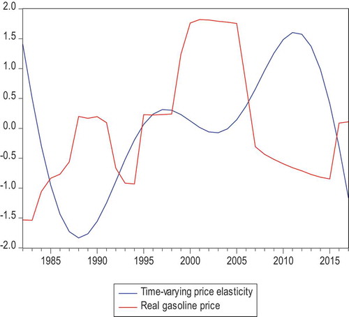
Figure 5 plots the time-varying price elasticity and real gasoline price data using a normalized scale. As can be seen from the figure, price elasticity moves in the opposite direction to the domestic price of gasoline. When the price of gasoline spiked sharply in 1988, price elasticity decreased to its lowest value (−0.31) in the period studied. Price elasticity began to increase the following year, following the decline in the gasoline price. The increase in the price of gasoline in 1995 by 72%, and its continued increase until 2002, is associated with the decline in the price elasticity until 2003. The gasoline price has declined in real terms since 2003, with the 2007 Royal decree (Al-Riyadh 2006) further accelerating this decline. The downward trend in the domestic price of gasoline price continued until 2015, while price elasticity increased until 2012. Price elasticity started to decline again as the gasoline price dropped in 2012. The Kingdom’s energy price reform of 2016 increased the domestic price of gasoline, and price elasticity further declined.

Scott’s (2012) finding that agents react more strongly to permanent price changes than temporary ones is evident from Figure 5: During the five-year periods of consecutive price increases (1984–1988 and 1997–2001), price elasticity fell to −0.31 in 1988 and −0.15 in 1999. However, though the gasoline price increased in 1995 by 72%, the price elasticity did not change significantly. This can be explained by the fact that the domestic price of gasoline declined in 1994 and 1996. The continued drop in gasoline prices in 2004–2011 saw price elasticity peak in 2011. The last gasoline price increase in 2016 also negatively impacted price elasticity. This could be due to (a) the gradual decrease in the growth rate of the price of gasoline, and (b) the cut in government transfers. This finding allows us to conclude that a sharp increase in the domestic price of gasoline after a period of permanent price increases, or followed by income ‘shrinking’ policies, might result in sizable changes in price elasticity in responses to this increase.

Lastly, the error correction model estimations show that income does not have a statistically significant impact on gasoline demand, replicating the findings of Atalla, Gasim, and Hunt (2018). The insignificant impact of income on gasoline demand in the short run in case of Saudi Arabia might be caused by the following factors: first, the saturation effect of driving. The unavailability of different transportation modes in Saudi Arabia makes driving a necessary good, which is bounded above (see Chang and Hsing 1991, inter alia). Second, Saudi Arabia is the fifteenth largest car market in the world, regularly renewing its car park (Motory 2018). Furthermore, as in other Gulf countries, luxury cars are very popular (Krane and Majid 2019). These cars are modern and are mainly fuel efficient, resulting in less gasoline consumption. Third, historically, the domestic price of gasoline has been very cheap. As such, the ability of consumers to purchase gasoline has been irresponsive to whether their incomes have been increasing or decreasing in the short-run.

The estimated short-run price elasticity is −0.13. It worth noting that Havranek, Irsova, and Janda (2012), reviewing the previous studies, concluded that the average short-run price elasticity of gasoline demand is −0.09, which is close to our finding.

Additionally, similar to Scott (2012), we found that price elasticity is more responsive to the permanent shocks/price changes. Our findings also support those of Gately (1992), in that high gasoline prices result in larger price responses, and low gasoline prices result in smaller responses.

8. Conclusion

Saudi Arabia, the biggest oil exporter is currently undergoing many socio-economic reforms including EPR. The success of these reforms requires better understanding of energy and macroeconomic linkages. The current paper investigates gasoline consumption, employing a time-varying coefficient cointegration approach. This approach allows us to analyze the varying responses of demand to income and price levels.

The following policy insights based on the findings of the paper can be pointed out.

Gasoline price increases, when prices are already high, cause larger negative impacts on gasoline demand. Policymakers may consider how this finding can inform energy efficiency measures: Price increases in higher price regimes could produce energy efficiency gains by curtailing gasoline demand.

Additionally, consecutive long-lasted price increases might cause demand to decrease severely. This finding could be useful for policymakers, depending on their objectives. For example, if they wish to increase energy efficiency, they could gradually increase prices over the long-term.

Moreover, the short-run income variations do not have a statistically significant impact on gasoline demand. This suggests that income support policies for the private sector, if required, should be designed considering their long-run impacts.

Overall, the policy insights mentioned above may be useful in the successful implementation of EPR and environmental policies.

Figure 1. Plots of variables.

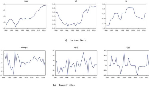
Figure 2. Time-varying income elasticity.

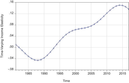
Figure 3. Time-varying price elasticity.

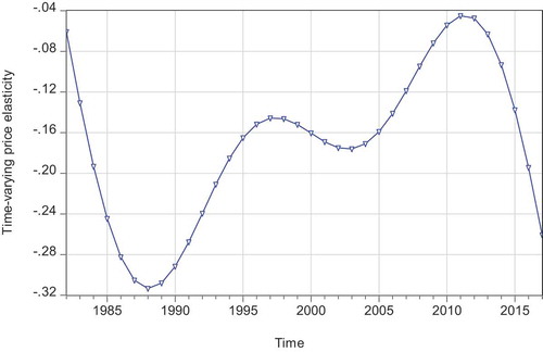
Figure 4. Comparison of income elasticity in different periods, with per capita income and government transfers (normalized scale).

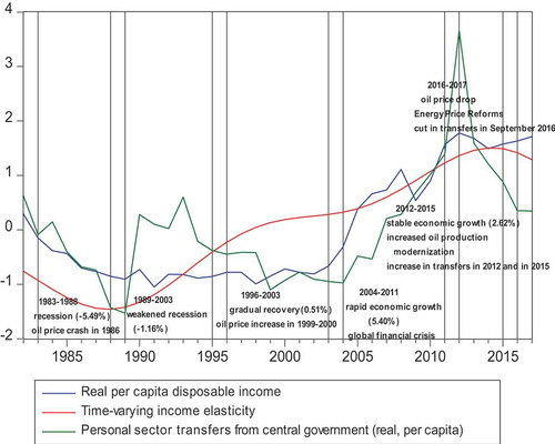
Figure 5. Time-varying price elasticity and gasoline price (normalized scale).

Acknowledgments

The authors would like to thank Fatih Karanfil, Walid Matar, Anwar Gasim, and Olivier Durand-Lasserve for their valuable comments and suggestions, which helped improve the quality of the paper. The views expressed in this paper are those of the authors and do not necessarily represent the views of their affiliated institutions. We also thank the attendants of the 21st Dynamic Econometrics Conference and especially to Sir David F. Hendry for their valuable comments.

Appendix A.

Figure 1A. Plots of (a) recursive residuals, (b) CUSUM and (c) CUSUM of squares tests for stability.

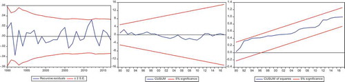
Table 1A. The ADF unit root test results.

	Variables	Level	k	First difference	k
Intercept	mgpt	-0.029	0	-2.667*	1
	rpt	-1.976	0	-4.553***	0
	dit	-0.211	0	-5.076***	0
Intercept and trend	mgpt	-2.957	2	-5.508***	0
	dit	-2.016	0	-5.950***	0
	rpt	-1.697	0	-4.616***	0

Notes: Maximum lag order is set to two and the optimal lag order (k) is selected based on Schwarz info criteria; ***, and * indicate a rejection of the null hypotheses at the 1% and 10% significance levels, respectively. The critical values are taken from MacKinnon (1996).

Table 2A. Cointegration test results.

Variable addition test
Distribution	Result	Critical values
Chi-square	test statistics	1%	13.18
df = 4	9.47	5%	9.49
		10%	7.78

Notes: df = degree of freedom. df is 4 as we used four trend variables for the VAT test.

Table 3A. Short-run final specification.

variables	ectt-1	d(incpt-1)	d(rpt)	d(mgpt-2)	d(dp1989)
coefficients	-0.766		-0.126	0.241	-0.103
p-values	(0.000)		(0.000)	(0.000)	(0.000)
	SE of Regression	R-squared	Log likelihood	df	k
	0.017	0.888	97.392	30	5
	LM test	White test	JB test	RESET test
	0.313	1.748	2.240	0.135
	(0.854)	(0.155)	(0.326)	(0.716)

Notes: ect = error correction term; SE of regression = standard error of regression; df = degree of freedom; k = number of observations; LM test=Breusch-Godfrey serial correlation LM test (lags = 2); White test = White test for heteroskedasticity; JB test = Jargue-Bera goodness-of-fit test; RESET test=Ramsey RESET test for misspecification.

References

- Ackah, I., and F. Adu. 2014. Modelling gasoline demand in Ghana: A structural time series approach. International Journal of Energy Economics and Policy 4 (1):76–82.
- Al Yousef, N. 2013. Demand for oil products in OPEC countries : A panel cointegration analysis. International Journal of Energy Economics and Policy 3 (2):168–77.
- Al-Awsat, A. 2019. Middle-east Arab news opinion. Accessed July 7, 2019. https://aawsat.com/english/home/article/1542696/saudi-aramco-announces-review-gasoline-prices-q1-2019.
- Al-Faris A., Abdula Razak F. 1992. Income and price elasticities of gasoline demand in the organization of Arab petroleum exporting countries. The Journal of Energy and Development. Accessed July 4, 2019 https://www.jstor.org/stable/24807631.
- Al-Faris, A. Razak. 1997. Demand for oil products in the GCC countries. Energy Policy 25 (1):55–61. doi:10.1016/S0301-4215(96)00122-X.
- Algunaibet, I. M., and W. Matar. December 2016. The responsiveness of fuel demand to gasoline price in passenger transport: A case study of Saudi Arabia. KAPSARC Discussion Paper. https://www.kapsarc.org/wp-content/uploads/2016/07/KS-1642-DP036A-The-Responsiveness-of-Fuel-Demand-to-Gasoline-Price-in-Passenger-Transport1.pdf.
- Al-Riyadh. 2006. Accessed June 16, 2019. http://www.alriyadh.com/211700 or http://www.alriyadh.com/150836#.
- Al-Sahlawi, M. A. 1988. Gasoline demand. The case of Saudi Arabia. Energy Economics 10 (4):271–75. doi:10.1016/0140-9883(88)90037-0.
- Al-Sahlawi, M. A. 1997. The demand for oil products in Saudi Arabia. OPEC Review 21 (1):33–38. doi:10.1111/1468-0076.00021.
- Alves, D. C. O., and R. L. S. Bueno. March, 2003. Short-run, long-run and cross elasticities of gasoline demand in Brazil. Energy Economics 25(2):191–99. doi: 10.1016/S0140-9883(02)00108-1.
- APICORP. 2018. Saudi energy price reform getting serious. APICORP Energy Research 3(5):3–5.
- Arzaghi, M., and J. Squalli. 2015. How price inelastic is demand for gasoline in fuel-subsidizing economies? Energy Economics 50:117–24. doi:10.1016/j.eneco.2015.04.009.
- Atalla, T. N., A. A. Gasim, and L. C. Hunt. 2018. Gasoline demand, pricing policy, and social welfare in Saudi Arabia: A quantitative analysis. Energy Policy 114 (March):123–33. doi:10.1016/J.ENPOL.2017.11.047.
- Bakhat, M., X. Labandeira, J. M. Labeaga, and L.-O. Xiral. 2017. Elasticities of transport fuels at times of economic crisis: An empirical analysis for Spain. Energy Economics 68 (October):66–80. doi:10.1016/j.eneco.2017.10.019.
- Baranzani, and Weber. 2013. Elasticities of gasoline demand in Switzerland. Energy Policy 63:674–680.
- Ben Sita, B., W. Marrouch, and S. Abosedra. 2012. Short-run price and in come elasticity of gasoline demand: Evidence from Lebanon. Energy Policy 46:109–115.
- Burke, P. J., and S. Nishitateno. 2013. gasoline prices, gasoline consumption, and new-vehicle fuel economy: Evidence for a large sample of countries. Energy Economics 36:363–70. doi:10.1016/j.eneco.2012.09.008.
- Campos F., J., N. R. Ericsson, and D. F. Hendry. August, 2005. General-to-specific modeling: An overview and selected bibliography. FRB International Finance Discussion Paper No. 838. doi:10.2139/ssrn.791684.
- Chakravorty U., F. Fesharaki, S. ZhouDomestic Demand for Petroleum in OPEC Countries. OPEC ReviewOrganization of the Petroleum Exporting Countries (2000)
- Chang, H. S., and Y. Hsing. 1991. The demand for residential electricity: New evidence on time-varying elasticities. Applied Economics 23 (7):1251–56. doi:10.1080/00036849100000165.
- Chang, Y., C. S. Kim, J. Isaac Miller, J. Y. Park, and S. Park. 2014. Time-varying long-run income and output elasticities of electricity demand with an application to Korea. Energy Economics 46:334–47. doi:10.1016/j.eneco.2014.10.003.
- Chang, Y., and Martinez-Chombo. 2003. Electricity demand analysis using cointegration and error-correction models with time varying parameters: The Mexican case. Working Paper 2003-08, Department of Economics, Rice University, Houston, TX, USA.
- Chang, Y., Y. Choi, K. J. Chang Sik, I. Miller, and J. Y. Park. 2016. Disentangling temporal patterns in elasticities: A functional coefficient panel analysis of electricity demand. Energy Economics 60:232–43. doi:10.1016/j.eneco.2016.10.002.
- Dahl, C., and T. Sterner. July, 1991. Analysing gasoline demand elasticities: A survey. Energy Economics 13(3):203–210.
- Dahl, C. A. 2012. Measuring global gasoline and diesel price and income elasticities. Energy Policy 41:2–13. doi:10.1016/j.enpol.2010.11.055.
- Dickey, D. A., and W. A. Fuller. 1981. Likelihood ratio statistics for autoregressive time series with a unit. Econometrica 49:1057. http://www.u.arizona.edu/~rlo/readings/278800.pdf.
- Eltony, M. N., and N. H. Al-Mutairi. 1995. Demand for gasoline in Kuwait: An empirical analysis using cointegration techniques. Energy Economics 17 (3):249–53. doi:10.1016/0140-9883(95)00006-G.
- Eltony, N. M. 1994. An econometric study of the demand for gasoline in the gulf cooperation council countries. The Journal of Energy and Development. Accessed July 4, 2019. https://www.jstor.org/stable/24808048.
- Eltony Nagy, M. 1996. Demand for gasoline in the GCC: An application of pooling and testing procedures. Energy Economics 18 (3):203–09. doi:10.1016/0140-9883(96)00011-4.
- European Commission, International Monetary Fund, OECD, United Nations, World Bank. 2008. “System of National Accounts.” Accessed July 4, 2019. https://unstats.un.org/unsd/nationalaccount/docs/SNA2008.pdf.
- Gately, D. 1992. Imperfect price reversibility of U.S. gasoline demand: Asymmetric responses to price increases and declines. Journal of Transportation and Statistics 2 (1):1–17.
- General Authority for Statistics (GaStat). 2017. National Accounts. Accessed July 7, 2019. https://www.stats.gov.sa/en.
- General Authority for Statistics (GaStat). 2018. Accessed July 7, 2019. https://www.stats.gov.sa/en.
- Gonand, F., F. J. Hasanov, and L. C. Hunt. 2019. Estimating the impact of energy price reform on Saudi Arabian intergenerational welfare using the MEGIR-SA model. The Energy Journal 40:3. doi:10.5547/01956574.40.3.fgon.
- Haas, R., and L. Schipper. 1998. Residential energy demand in OECD-countries and the role of irreversible efficiency improvements. Energy Econ 20:421–42. doi:10.1016/S0140-9883(98)00003-6.
- Havranek, T., and O. Kokes. 2015. Income elasticity of gasoline demand: A meta-analysis. Energy Economics 47:77–86. doi:10.1016/j.eneco.2014.11.004.
- Havranek, T., Z. Irsova, and K. Janda. 2012. Demand for gasoline is more price-inelastic than commonly thought. Energy Economics 34 (1):201–07. doi:10.1016/j.eneco.2011.09.003.
- Hemrit, Wael& Noureddine Benlagha, 2018. “The impact of government spending on non-oil-GDP in Saudi Arabia (multiplier analysis),” International Journal of Economics and Business Research, Inderscience Enterprises Ltd, vol. 15(3), pages 350–372. https://doi.org/10.1504/IJEBR.2018.10011597
- Hössinger, R., C. Link, A. Sonntag, and J. Stark. 2017. Estimating the price elasticity of fuel demand with stated preferences derived from a situational approach. Transportation Research Part A 103 (2017):154–71.
- International Energy Agency (IEA). 2018. Extended world energy balances.
- Joint Organisations Data Initiative Oil (JodiOil). 2018. Improving global oil data transparency. Accessed July 4, 2019. https://www.jodidata.org/oil/.
- Park, J. Y., and S. B. Hahn. 1999. Cointegrating regressions with time varying coefficients. Economic Theory 15:664–703. doi:10.1017/S0266466699155026.
- Krane, J., and Majid F. Women driving in Saudi Arabia: ban lifted, what are the economic and health effects? Accessed July 4, 2019. https://www.bakerinstitute.org/media/files/files/564007c9/bi-brief-061318-ces-chb-saudiwomendriving.pdf.
- Lin, C.-Y. C., and L. Prince. 2013. Gasoline price volatility and the elasticity of demand for gasoline. Energy Economics 38 (2013):111–17. doi:10.1016/j.eneco.2013.03.001.
- MacKinnon, J. G. 1996. Numerical distribution functions for unit root and cointegration tests. Journal of Applied Econometrics 11 (6):601–18. doi:10.1002/(SICI)1099-1255(199611)11:6<601::AID-JAE417>3.0.CO;2-T.
- Manzan, S., and D. Zerom. 2010. A semiparametric analysis of gasoline demand in the united states reexamining the impact of price. Econometric Reviews 29 (4):439–68. doi:10.1080/07474930903562320.
- Mikayilov, J. I., F. J. Hasanov, C. A. Bollino, and C. Mahmudlu. 2017. Modeling of electricity demand for Azerbaijan: Time-varying coefficient cointegration approach. Energies 10:11. doi:10.3390/en10111918.
- Mikayilov, J. I., F. J. Hasanov, and M. Galeotti. 2018. Decoupling of CO2 emissions and GDP: A time-varying cointegration approach. Ecological Indicators 95 (December):615–28. doi:10.1016/J.ECOLIND.2018.07.051.
- Mikayilov, J. I., F. J. Hasanov, W. Olagunju, and M. H. Al-Shehri. July, 2020b. Electricity demand modeling in Saudi Arabia: Do regional differences matter? The Electricity Journal 33(6):106772. doi: 10.1016/j.tej.2020.106772.
- Mikayilov, J. I., S. Mukhtarov, and J. Mammadov. 2019b. Income and price elasticities of gasoline demand: An empirical analysis for Russia. ASERC Journal of Socio-Economic Studies 1:2.
- Mikayilov, J. I., S. Mukhtarov, and J. Mammadov. 2020a. Gasoline demand elasticities at the backdrop of the lower oil prices: Fuel-subsidizing country case. Energy Economics. Under review.
- Motory 2018. Saudi Arabia Is the 15th largest car market in the world. https://ksa.motory.com/en/news/saudi-arabia-is-the-15th-largest-car-market-in-the-world-1087/.
- Mousavi, M. H., and S. Ghavidel. June, 2019. Structural time series model for energy demand in Iran’s transportation sector. Case Studies on Transport Policy 7 (2):423–32.
- Neto, D. 2012. Testing and estimating time-varying elasticities of Swiss gasoline demand. Energy Economics 34 (6):1755–62. doi:10.1016/j.eneco.2012.07.009.
- Osman, T., and D. Ayhan. 2016. Forecasting and analysis of energy consumption for transportation in the kingdom of Saudi Arabia. Energy Sources, Part B: Economics, Planning, and Policy 11 (12):1150–57. doi:10.1080/15567249.2015.1004383.
- Park, J. Y. 1992. Canonical cointegrating regressions. Econometrica 60:119–43. doi:10.2307/2951679.
- Park, J. Y., K. Shin, and Y. Whang. 2010. A semiparametric cointegrating regression: Investigating the effects of age distributions on consumption and saving. Journal of Econometrics 157 (2010):165–78. doi:10.1016/j.jeconom.2009.10.032.
- Park, S. Y., and G. Zhao. 2010. An estimation of U.S. gasoline demand: A smooth time-varying cointegration approach. Energy Economics 32 (1):110–20. doi:10.1016/j.eneco.2009.10.002.
- Park, J. Y. 1990. Testing for unit roots and cointegration by variable addition. In Advances in econometrics, ed. 8, pp. 107-133.
- PricewaterhouseCoopers (PwC). 2018.Women driving the transformation of the KSA automotive market. https://www.pwc.com/m1/en/publications/documents/women-driving-the-transformation-of-the-ksa-automotive-market.pdf.
- Ramakrishnan, R., and S. Geetha. 2006. A study of the patterns of production and consumption of crude oil and petroleum products in the sultanate of Oman. Energy Sources, Part B: Economics, Planning, and Policy 1 (1):37–53. doi:10.1080/009083190892975.
- Scott, K. R. 2012. Rational habits in gasoline demand. https://doi.10.1016/j.eneco.2012.02.007.
- Thomas, G. K. 2011. The consumer response to gasoline price changes : Empirical evidence and policy implications. Stanford Digital Repository. Accessed July 4, 2019. https://purl.stanford.edu/wz808zn3318.
- Totto, L., and T. M. Johnson. 1983. OPEC domestic oil demand: Product forecasts for 1985 and 1990. OPEC Review 7 (2):190–227. doi:10.1111/j.1468-0076.1983.tb00260.x.
- United Nations (UN). 2017. United Nations Population Database.