An integrated mixed integer linear programming model for resilient and sustainable natural gas supply chain

ABSTRACT

Disruptions in the natural gas supply chain result in reduced throughput and associated emissions and losses, causing significant economic, environmental, and social impacts. Therefore, it is crucial to design supply chains that are resilient and sustainable to prevent or reduce the effects of disruptions. This paper proposes a novel Mixed-Integer Linear Programming model, which optimizes the natural gas supply chain in terms of resilience and sustainability, by examining the impact of an additional workflow design (contingency pipeline) located between the shutdown inlet and outlet nodes in the transmission echelon. The model is applied to a “real world” case, using data collected from gas companies operating in Nigeria. Both steady and transient states of the system are examined in this study through a set of scenarios. The best final solution was found to yield 93.6% performance increase when compared to target throughput and 63% performance increase with the introduction of the contingency when compared with the baseline scenario.

KEYWORDS:

• Natural gas
• Supply chain
• Optimization
• Mixed-integer linear programming
• Resilience
• Sustainability

Introduction

Climate change concerns have led Governments around the globe to adopt legally binding commitments to cut down their greenhouse gas (GHG) emissions to limit the global warming effects (UNFCCC 2015). Today’s society confronts the significant challenge of providing sustainable energy to meet the growing global demand (British petroleum 2019). In 2019, the energy consumption increased by 1.3% in relation to 2018, representing less than half of the 2.8% growth in 2018; the increase in consumption was met mainly by Natural Gas (NG) and renewables (British Petroleum 2020). NG is a significant player in the energy mix and a reliable energy fuel that has been reported to bridge the gap between conventional and renewable sources (Hamedi et al. 2009; Mac, Brouwer, and Scott Samuelsen 2018). Projections of the future global energy mix suggest that 85% of total energy supply growth will be generated by NG and renewables, with renewables becoming the largest power generation by 2040 (British petroleum 2019). The NG-fired power plant is a relatively low-carbon, flexible technology, which can be used to enable a low carbon energy transition (Ríos-Mercado and Borraz-Sánchez 2015; Sayed, Wang, and Bi 2019). Although NG is associated with strong GHG emissions at different supply chain levels, it is argued that it generates less emissions compared to other fossil fuels and promotes cleaner production (Balcombe, Hawkes, and D 2018; Emenike and Falcone 2020; Hao et al. 2016; Zhang et al. 2020). Furthermore, flexible NG-fired power plants can satisfy changes in peak demand and network congestions, resulting from intermittent renewable energy (such as wind and solar) in the network, challenging the power system security (Hutagalung et al. 2017; Ioannou et al. 2019).

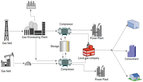
The NG supply chain consists of several interconnected nodes (see Figure 1), composed of supply, transmission, distribution, compression, storage, and production sectors (interconnected by physical and financial infrastructure, information sharing, and conveyance) rendering the system broad and complex, like other major energy supply chain systems (Kinnon, Brouwer, and Samuelsen Mac, Brouwer, and Scott Samuelsen 2018). In addition to the system’s complexity, multiple parties usually manage individual components, posing challenges to the management of the network.

Figure 1. Simple layout of a natural gas supply chain.

The NG supply chain is exposed to disruptions, resulting in reduced throughput and increased associated costs and emissions (Emenike and Falcone 2020). Disruptions in the NG supply chain can lead to a prolonged compressor and pipeline shutdown (Carvalho et al. 2012). Common causes of disruptions to the energy supply chain system include: infrastructure failure, routine or emergency shutdown, human attack, natural disaster, theft, unexpected delay, queuing, demand variation, inventory shortage, inefficient supply capacity, and political upheaval (Lee and Han Kim 2002). Indeed, high levels of identifiable risks (Doukas, Flamos, and Psarras 2011), long lead-times, insufficient communication between nodes, and single supply sources are undesirable characteristics in a supply chain.

Improvements in the physical infrastructure, telecommunications, business environment, project cost, and efficiency can generally address the above shortcomings. This study focuses on the optimization of the physical infrastructure of the NG transmission network toward increased resilience and environmental sustainability. A sustainable NG supply chain aims at reducing the negative impact on the environment, business, and people. The concept of resilience refers to the capacity to bringing the system back to its original or more desirable state following a disruption (Christopher and Peck 2004; Hoggett 2014). Some of the resilient strategies that have been adopted over the years include multiple sourcing, introduction of backup facilities and suppliers and use of additional inventory/storage, among others. Optimization is useful to achieve resilience in the NG supply chain, addressing the occurrence of disturbances and their potential impacts (Emenike and Falcone 2020).

Most studies on the optimization of the NG supply chain emphasize the minimization of the system cost or profit maximization as objective functions (El-Shiekh 2013). For instance, Zarei and Amin-Naseri (2019) designed and optimized an integrated NG supply chain formulated as a MILP model that minimizes total cost. The model provides the optimized NG flow between supply chain nodes, their capacities, number of pipelines, capacity expansion, extraction, production, storage, exports, and imports. Following a sensitivity analysis of the model, results indicated that the highest impact parameters on the optimal solution are the operating costs and the demand. Another study focused on the design of NG transmission networks using a two-objective optimization framework, namely the minimization of the transportation tariff and the maximization of the transported gas volume, with gas flow and compressor stations (Alves, de Souza, and Luiz Hemerly Costa 2016). Apart from cost minimization and profit maximization, researchers have investigated key objectives such as portfolio diversification, flexible contracts, capacity planning for transportation, safety stocks, and system redundancy (Emenike and Falcone 2020). These objective functions can promote the flexibility and resilience of the NG supply chain process. Emenike and Falcone (2020) stated that optimizations have been carried out on different levels of the supply chain echelon due to the complexity of the NG supply chain. Generally, NG optimizations are mostly evaluated on the transportation level involving the pipeline and compressor nodes (Abahussain and Christie 2013; Bopp et al. 1996; Farzaneh-Gord and Rahbari 2016; Sabri and Beamon 2000; Vasconcelos et al. 2013).

The transportation pipeline network is a complex, large-scale optimization problem with inherent nonlinearities, including, for example, the flow pressure loss constraints, and other hydraulic equations (Humpola and Fügenschuh, 2015). Several authors have developed models to simulate the nonlinear dynamics of the gas networks. Zhou et al. (2021) developed a Mixed-Integer Nonlinear Programming (MINLP) model for an underground pipeline network of gas storage (UNGS) that aimed at minimizing the total cost of pipelines, platforms, and stations. Considering the flow conditions of injection and production, the algorithm finds the best pipe network layout, the topology of the platform and the central station, and the pipe diameters of the ground pipe network of the system. Humpola and Fügenschuh (2015) used a MINLP model to study a pipe network design problem, which considered nonlinear and nonconvex potential-flow coupling constraints to define the relationship between the flow rate at an arc and the pressure at the end nodes. Kabirian and Hemmati (2007) developed a strategic planning model for natural gas networks such that the optimization of the nonlinear model addresses the short-run development plan where the location of compressor stations, pipeline routes, and sources of natural gas was considered to reduce transmission network cost while meeting increasing energy demand. Also, to improve the active control for gas transmission systems Sukharev and Kosova (2017) considered the problem associated with technical parameter identification in an unsteady state using a nonlinear model. Similarly, Mikolajková et al. (2017) developed a model of a pipeline network for NG distribution through a multi-period MINLP formulation, using the overall system cost, including fuel costs, investment and operation costs as the objective function. Constraints of the model included mass and energy balance for the network nodes, pressure drop equations, and gas compression in compressor nodes.

Nevertheless, such design optimization problems can become very computationally intricate. To address this, Hong et al. (2020) developed an integrated MILP method to derive the optimal gathering pipeline network, by considering the minimization of total construction cost as the objective function and using a piecewise method to linearize the nonlinear hydraulic equations. Zhang et al. (2017) also developed an integrated MILP method to derive the optimal production well gathering pipeline network toward minimizing the total investment while considering terrain, obstacles, and other constraints.

Disruptions in the NG supply chain can cause significant economic, environmental, and social impacts (Emenike and Falcone 2020) and a number of scholars have studies the design of resilient supply chains to prevent or reduce the effects of disruptions. Carvalho et al. (2014) studied the design of the NG supply chain aiming at reducing the impact of disruption due to factors outside the control of the business. The researchers proposed a decentralized method toward NG network resilience to failures when disruption occurs. Three strategies to manage congestions from disruptions were identified: network expansion, implementation of congestion pricing to cap the consumption of heavy users that cause network bottlenecks, and the grouping of consumers with similar suppliers’ dependencies. One of the pinch points is the pipeline as it limits the quantity of flow based on its capacity available for NG transportation. The pipeline can also be affected by leakage or shutdown at the compressor station. To adopt a performance measurement, a new index that evaluates the functionality of a NG distribution network was proposed. It involved the restoration process after the occurrence of an external disruption, using recovery time as the main factor (Cimellaro, Villa, and Bruneau 2015). Focusing on the restoration problem of an interdependent infrastructure network following the occurrence of a disruptive event and the different interruption scenarios, Yasser, Barker, and Albert (2019) devised a resilience-driven restoration model to tackle and restore the system to normal state. Four key factors to be minimized were considered in the model, namely, the restoration time and the total cost as the sum of flow cost, restoration cost, and disruption cost (i.e., unmet demand cost). A decentralized algorithm model that controlled congestion in the NG supply chain affected by disruption, was proposed by (Carvalho et al. 2014). The model ensured that the available network capacity is distributed to each route without reducing network throughput. The approach considered a wide range of scenarios on a country-by-country basis within Europe and adopted a mitigation strategy. Specific indices were introduced to verify the results, based on per capita throughput and coefficient of throughput variation. The supply chain’s resilience has attracted the attention of industry experts and researchers due to its considered competitive advantage (Balcombe, Hawkes, and D 2018; Christopher and Peck 2004; Moslehi and Reddy Pourhejazy et al. 2017).

This study presents a Mixed-Integer Linear Programming (MILP) framework for optimizing the resilience and environmental sustainability of a NG supply chain. To this end, the proposed model examines the impact of a relief pipeline contingency employed to address the unplanned disruption to a network and its subsequent closure. Compared to existing literature related to the NG supply chain optimization, the novelty of this paper lies on, firstly, the modeling of the impact of a relief pipeline redundancy on the NG supply chain as part of the mitigation planning problem (MPP) and secondly on the integration of resilience and environmental sustainability objectives in the proposed Mixed Integer Linear Programming (MILP) model.

The rest of the paper is structured as follows. In Section 2, the definition of the problem, model assumptions, and the overview of the scenarios investigated are presented. Section 3 outlines the mathematical programming model. In Section 4, the case study, composition of the infrastructure and the overview of the NG-proposed workflow are described. Section 5 describes the results generated in the steady and transient states. Finally, Section 6 presents the concluding remarks and discussion.

Problem definition

This study addresses the mitigation planning problem (MPP) of a natural gas supply chain by optimizing a relief pipeline contingency employed to address the unplanned disruption of the network. Disruption and subsequent shutdown of the compressor node results in emission losses, downtime, and shortage in throughput supply. Excess trapped NG in the mainline supplying the compressor station is usually emitted, inducing an environmental threat because of continuous flow from upstream. The NG network’s initial performance describes the known operating state; the optimization model is then applied to study the impact of the disruption.

The main features and assumptions of the proposed MILP model are summarized as follows (the list of symbols can be found in the Nomenclature):

• The given planning horizon is divided into equal time intervals $t\text{isin}T$ over a period of 30 months.

• The inlet nodes can include the supplier $(i)$, the processing plant $j)$, the compressor $(k)$, and the city gate $(g)$ nodes.

• Outlet nodes can include the processing plant $(j)$, the compressor $(k)$, the city gate $(g)$ and the consumer $(q)$ nodes.

• Shutdown and startup periods $t\in T$ are defined for every node $k$. During shutdown period, $t$, there is a loss of gas represented as $Z_{\left(t\right)}^E$. The startup is defined as the time the plant requires to start running, featured as $Y_{\left(k,t\right)}$ Shutdown is denoted as $R_{\left(k,t\right)}$, while the operating time is represented as $X_{\left(k,t\right)}$.

• The demand volume for consumer, $d\mathrm{\_}{a}_{\left(m,t\right)}$, is associated with a dedicated capacity, $r{c}_{\left(m,t\right)}^{max}$.

• During the shutdown, $R_{\left(k,t\right)}$ the loss $Z_{\left(t\right)}^E$ through emissions is recorded for a time duration.

• The impact of disruption on the gas flow to the plant is bounded by the minimum $S_{\left(k\right)}^{min}$ and maximum $S_{\left(k\right)}^{max}$ mass flow rates.

• The nodes from the supplier to the consumers are interconnected. There are no dedicated storage units. Pipelines provide limited temporary storage for every given time.

• It is assumed that no more than two plants are simultaneously shutdown.

• Disruption to the network nodes is identified as the main cause for the shortfall in supply. In steady state, the pipelines are operating at constant flow rates with a constant pressure profile, which may differ from point to point, but does not change with time (Menon 2005). In this work, The General Flow Equation (GFE) for the steady state isothermal flow in a gas pipeline is introduced, which is the basic equation of the pressure drop as a function of the flow rate. If the inlet pressure at the upstream is constant in the steady state, the flow rate will increase if the downstream outlet pressure is reduced. The pressure drop was modeled following Menon’s (2005) equation as follows:

  $X=77.54\cdot \left(\frac{T_b}{P_b}\right)\cdot {\left(\frac{P_1^2-P_2^2}{G{T}_{f}LZf}\right)}^{0.5}\cdot D^{2.5}$

where f=friction factor

P_b=base pressure

P₁=upstream pressure

P₂=downstream pressure   

G=gas gravity, (air = 1.00)

T_f=average gas flowing temperature (°R (460+°F))

L=pipe segment length

Z=gas compressibility factor at the flowing temperature (dimensionless)

D=pipe inside diameter

• The initial state of the network is static except for the introduced relief pipe, while the dynamic state of the system is also studied.

• The different statuses of the plant nodes include the following: operational, shutdown or start up.

Overview of the NG network model and alternative pathway (relief pipeline) component

An overview of the NG supply chain infrastructure with the additional workflow (pipeline redundancy) is shown in Figure 2. A detailed description of the system can be found in Emenike and Falcone (2020). The relief pipeline is located in the midstream between the gas processing plant and the distribution center (red colored line). The city gate station (CGS) regulates the natural gas (NG) pressure by using expansion valves (Sheikhnejad, Simões, and Martins 2020).

Figure 2. Case study system layout with additional workflow (adopted from (Emenike and Falcone 2020)).

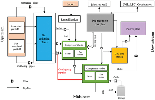
When the emergency shutdown occurs, the gas flows through emergency outlet between the valve and the compressor station. Without this relief pipeline, the gas is emitted through a relief valve to the environment, resulting in throughput losses and pollution to the environment. This relief pipe gradually flows the gas to a sale line or to another compressor station depending on its proximity to the sale line.

The introduction of the relief pipe is to ensure continuous flow and help the network withstand the impact of the disruption. The relief pipeline takes the excess flow during shutdown so that the pressure at the end does not increase excessively, leading to a reverse flow (where the pressure at the end of the pipe is greater than that at the inlet). The mathematical model describing the necessary conditions for the optimization process is presented in Section 3.

If the flow is constant in time and the pipeline is straight and horizontal, then according to Tomasgard et al. (2007), it can be assumed that the system is in steady state, and the time resolution is strategic or tactical and not operational.

Overview of scenarios investigated

Table 1 summarizes all optimization scenarios implemented in Section 5. The baseline scenario (BS) is used to benchmark the compressor’s performance and throughput without introducing the relief pipeline (emergency outlet). The mean throughput of the BS constitutes a key performance indicator used to compare the scenarios. The redundancy (relief pipeline) is introduced in the other scenarios, and it is set to operate only when the disruption occurs. In scenario 1, the redundancy is introduced through the opening of the alternative pathway valve, allowing the flow into the alternative pathway in the steady state. Scenario 2 introduces flow constraints in an extended time-series to investigate the impact of flow constraint when the redundancy is operating. Scenario 3 comprises the extended time-series without the flow constraint. The extended time-series in scenarios 2 and 3 is required to forecast future data points in the planning horizon and to eliminate possible deviance in the data. Two scenarios are analyzed under the transient state. Scenario 4 analyses pressure variation resulting in pressure surge from the plant closure, while scenario 5 analyses the prolonged closure in both the inlet and outlet nodes on the mainline. The scenarios in both steady and transient states are summarized in Table 1.

Table 1. Optimization scenarios.

Scenario	Description	Condition
Steady state
0	Baseline scenario	No relief pipeline
1	Shutdown with redundancy	Relief pipeline operating with no pressure variation
2	Flow constraint in extended time	Flow constraint introduced when redundancy is operating
3	No flow constraint in extended time	No corresponding upper & lower bound limits
Transient state
4	Pressure surge from plant closure	Trapped gas undergoes pressure variation
5	Prolonged inlet & outlet nodes closure	Unexpected pressure build-up

Mathematical programming model

A mixed integer linear mathematical programming model is adopted in this work. GAMS mathematical programming system for optimization supports interfaces with several optimization algorithms or solvers. The GAMS programming model is considered a reliable optimization tool for mathematical modeling of the supply chain, where the run time varies based on the objective to be achieved.

Model Formulation

In this section, the MILP optimization model describing the gas supply chain with the disruption and loss elements is introduced, along with the alternative pathway that can serve as a capacity for expansion. The optimized model formulation aims to make the supply chain more resilient and sustainable. The detailed list of symbols used in the paper can be found in the Nomenclature.

Objective function

The objective of the optimization problem is to maximize the resilience of the supply of NG using flow volume flexibility from supplier to consumer nodes and minimize the associated emissions during plant shutdown. In the context of this study, the resilience has been approximated through the minimization of the throughput losses of the supply chain system. The flexibility of the supply chain nodes will help achieve the targeted resilience. For simplification, the multi-objective optimization problem has been formulated as a single-objective function, which is composed of the aggregate volume flexibility as a function of flow (represented as Z1), as well as the losses and emission savings, the operating status of the plant, and the additional flowline (Z2). The same weight was applied to all individual items of the objective function. As such, the objective function can be expressed as:

(1) $Maxf=\stackrel{Z1}{\overbrace{\left(SVF\right)+\left(PVF\right)+\left(TVF\right)}}+\stackrel{Z2}{\overbrace{\left(OS\right)+\left(AF\right)+\left(SIF\right)-\left(LES\right)}}=\left({\displaystyle \sum _{i,j,t}{g}_{\left(i\right)}^{max}}Z{A}_{\left(i,j,t\right)}{\epsilon }_{\left(k\right)}\right)+\left({\displaystyle \sum _{j,k,t}{h}_{\left(j\right)}^{max}}X\_P_{\left(j,k,t\right)}\right)+({\displaystyle \sum _{k,g,m,t}{s}_{\left(k\right)}^{max}}Y\_F_{\left(k,g,t\right)}+Y\_W_{\left(k,m,t\right)}+{\displaystyle \sum _{k,m,t}Y}\_W_{\left(k,m,t\right)}m{c}_{\left(k\right)}^{max}+{\displaystyle \sum _{k,g,t}Y}\_F_{\left(k,g,t\right)}m{c}_{\left(k\right)}^{max}+\left({\displaystyle \sum _{k,t}{\Psi }_{\left(k\right)}}{Y}_{\left(k,t\right)}+{\delta }_{\left(k\right)}{R}_{\left(k,t\right)}\right)+\left({\displaystyle \sum _{k,z,t}{v}_{\left(z\right)}^{max}}R\_F_{\left(k,z,t\right)}+{\delta }_{\left(\kappa \right)}\right)\left({\displaystyle \sum _{k,w,t}{s}_{\left(k\right)}^{max}}Y{M}_{\left(k,w,t\right)}^{+}-Y{M}_{\left(k,w,t\right)}^{-}\right)-\left({\displaystyle \sum _{kt}{O}_{\left(k\right)}}{Z}_{\left(t\right)}^E\right)$(1)

Where,

• Supply node volume flexibility (SVF), which corresponds to the maximum inlet flow from the supplier to the processing plant multiplied by the mass flow rate (from node $i$ to $j$ in time $t$). This ensures that the amount of product from the supply node is within the capability of the processing plant node.

• Processing node volume flexibility (PVF), which corresponds to the maximum inlet flow from the processing plant to the compressor multiplied by the mass flow rate (from node $j$to $kin$ time $t$). This ensures that the amount of product transported from the processing plant node is within the capacity of the compressor node.

• Transmission node volume flexibility (TVF), which corresponds to the maximum inlet flow from the compressor plant to the consumer node multiplied by the mass flow rate. This is a function of node k, m and g multiplied by maximum pressure in the compressor. This ensures that the amount of product from the compressor node is within the capacity of the consumer node.

• Operating status (OS), which corresponds to the operating status of the plant with respect to the minimum run time after startup and the minimum shutdown time.

• Additional flowline (AF), which corresponds to the flow to relief pipe from the main line during shutdown multiplied by the maximum flow rate. This describes the redundancy introduced to mitigate the impact of the shutdown.

• Storage inventory flowline (SIF), which corresponds to the flow to the storage inventory minus the flow from the storage inventory.

• Losses and emissions (LES), where the decision variable ($Z_{\left(t\right)}^E$) denotes the total amount of losses caused by the shutdown per time unit, multiplied by the shutdown time parameter (${\mathrm{O}}_{\left(\mathrm{k}\right)}$).

Constraints

Supplier capacity constraint

The supplier node represents the gas fields, which is often owned by multiple parties with production rights to produce in commercial quantities. Constraint (2) ensures that the supplied NG to the production plant is less than or equal to the supply capacity and the production plant capacity (Zhou, 2021). The total NG volume from all related gas wells does not exceed the maximum production capacity of gas fields in the supply node$i$, as shown in constraint (3):

(2) $\sum _{j\in J}Z{A}_{\left(i,j,t\right)}\le s{c}_{\left(i,t\right)}^{max},\mathrm{\forall }t\in T,i\in I$(2)

(3) $\sum _{i\in I}Z{A}_{\left(i,j,t\right)}\le j{c}_{\left(j,t\right)}^{max},\mathrm{\forall }t\in T,j\in J$(3)

Compressor capacity constraint

The compressor is one of the vital nodes in the gas network system. It is used throughout the natural gas network to move gas from the upstream to the midstream and finally to the downstream at different pressures. It helps to exert pressure that has been lost due to friction in gas pipelines (Menon 2005) and to reduce volume by providing the necessary force to move the gas along the pipeline. Constraints (4) and (5) ensure that NG flow from the processing plant node, $j,$ to the compressor node,$k$, minus the gas losses and emissions at time, $t$, do not exceed the compressor capacity. The shutdown of plant node $k$ is taken into consideration when there is a flow from plant $j$to plant $k$ to account for the losses during plant disruption. Constraint (6) ensures that if node $k$ supplies to the consumers, capacity must not exceed that of plant node $k$. The constraint is represented below:

(4) $\sum _{w\in W}Y{M}_{\left(k,w,t\right)}^{+}-Y{M}_{\left(w,k,t\right)}^{-}+\sum _{j\in J}{X}_{P_{\left(j,k,t\right)}}-Z_{\left(t\right)}^E\le c{p}_{\left(k,t\right)}^{max},\mathrm{\forall }t\in T,k\in K$(4)

(5) $\sum _{j\in J}X\mathrm{\_}{P}_{\left(j,k,t\right)}-emission{s}_{\left(k,t\right)}\le c{p}_{\left(k,t\right)}^{max},\mathrm{\forall }t\in T,k\in K$(5)

(6) $\sum _{m\in M}Y\mathrm{\_}{W}_{\left(k,m,t\right)}+\sum _{g\in G}\sum _{n\in N}Y{C}_{\left(g,n,t\right)}+Y{P}_{\left(g,n,t\right)}\le c{p}_{\left(k,t\right)}^{max},\mathrm{\forall }t\in T,k\in K$(6)

Power plant capacity constraint

In constraint (7), the power plant is being supplied directly from plant node $k$. In this constraint, it is expected that NG flow from the plant node $k$ to the transmission pipeline does not exceed the power plant capacity. It is assumed that the shutdown of plant node $k$ affects primarily the supply of NG to the power plant.

(7) $\sum _{k\in K}Y\mathrm{\_}{W}_{\left(k,m,t\right)}\le r{c}_{\left(m,t\right)}^{max},\mathrm{\forall }t\in T,m\in M$(7)

City gate station capacity constraint

The city gate is a point at which a local gas utility receives gas from a transmission system. It supplies gas to the customers in the city at required consumption pressure. When the city gate station is opened, all NG flow from compressor node, $k,$ in the transmission pipeline should not exceed the city gate capacity. This is ensured in constraint (8).

(8) $\sum _{k\in K}Y\mathrm{\_}{F}_{\left(k,g,t\right)}\le ph{i}_{\left(g,t\right)}^{max},\mathrm{\forall }t\in T,g\in G$(8)

Consumer demand constraint

Based on the contractual agreement at every time period, consumers’ demand should be satisfied by the suppliers as shown in constraints (9) – (11).

(9) $\sum _{k\in K}Y\mathrm{\_}{W}_{\left(k,m,t\right)}=d_{a_{\left(m,t\right)}},\mathrm{\forall }m\in M,\mathrm{\forall }t\in T$(9)

(10) $\sum _{g\in G}Y{P}_{\left(g,n,t\right)}=d_{b_{\left(n,t\right)}},\mathrm{\forall }n\in N,\mathrm{\forall }t\in T$(10)

(11) $\sum _{g\in G}Y{C}_{\left(g,q,t\right)}=d_{c_{\left(q,t\right)}},\mathrm{\forall }q\in Q,\mathrm{\forall }t\in T$(11)

Storage capacity constraint

Constraints (12) – (14) suggest that the upper and lower limits of the temporary storage capacity should not be surpassed. In constraints (12) and (13), the gas sent to the pipeline for storage should be less than or equal to the capacity of the line packing storage capacity. Constraint (14) represents the minimum and maximum inventory storage levels, i.e., it indicates that the gas storage must fall between its minimum and maximum limits. The parameter $y_{\left(w,t\right)}^S$ represents the initial inventory in the storage, while the variables $Y{M}_{\left(k,w,t\right)}^{+}$ and $Y{M}_{\left(w,k,t\right)}^{-}$ are the inflows and outflows from and to the compressor and the storage.

(12) $\sum _{k\in K}Y{M}_{\left(k,w,t\right)}^{+}+Y{M}_{\left(w,k,t\right)}^{-}\le s{t}_{\left(w,t\right)}^{max},\hspace{0.17em}\mathrm{\forall }\mathrm{t}\in \mathrm{T},w\in W$(12)

(13) $\sum _{\mathrm{k}\in \mathrm{K}}{\mathrm{Y}\mathrm{M}}_{\left(\mathrm{k},\mathrm{w},\mathrm{t}\right)}^{+}\le {\mathrm{s}\mathrm{t}}_{\left(\mathrm{w},\mathrm{t}\right)}^{\mathrm{m}\mathrm{a}\mathrm{x}}-{\mathrm{y}}_{\left(\mathrm{w},\mathrm{t}\right)}^{\mathrm{S}}\hspace{0.17em},\mathrm{\forall }\mathrm{t}\in \mathrm{T},\mathrm{w}\in \mathrm{W}$(13)

(14) $s{t}_{\left(w,t\right)}^{max}\ge {B_S}_{\left(w,t\right)}\ge s{t}_{\left(w,t\right)}^{min},\mathrm{\forall }t\in T,\mathrm{w}\in \mathrm{W}$(14)

Material input–output balance constraint

In constraint (15), as there is no mass buildup in any node of the network, each node will be constrained according to the mass balance law (Zhou et al., 2021). Thus, for every node of the network system: $\sum flowin=\sum flowout$. NG supplied from the gas fields to the processing plant equals NG transmitted from the processing plant to the compressor:

(15) $\sum _{i\in I}\sum _{j\in J}Z{A}_{\left(i,j,t\right)}=\sum _{j\in J}\sum _{k\in K}X\mathrm{\_}{P}_{\left(j,k,t\right)},\mathrm{\forall }t\in T$(15)

Furthermore, the total NG supplied from the processing plant to the compressor and from the compressor should equal the NG from the compressor to the power plant and from the compressor to the city gate station, as shown in constraint (16).

(16) $\begin{array}{rl}& \sum _{j\in J}\sum _{k\in K}X\mathrm{\_}{P}_{\left(j,k,t\right)}-Z_{\left(t\right)}^E+\sum _{w\in W}\sum _{k\in K}Y{M}_{\left(w,k,t\right)}^{-}\\ & =\sum _{\kappa \in K}\sum _{m\in M}Y\mathrm{\_}{W}_{\left(k,m,t\right)}+\sum _{k\in K}\sum _{w\in W}Y{M}_{\left(k,w,t\right)}^{+}\\ & +\sum _{g\in G}\sum _{k\in K}Y\mathrm{\_}{F}_{\left(k,g,t\right)},\mathrm{\forall }t\in T\end{array}$(16)

The local distribution company (LDC) oversees the operation of the city gate station. Constraint (17) shows that the NG supplied from the compressor to the gas company equals the NG supplied from the gas company to the industrial and domestic consumers:

(17) $\sum _{\kappa \in K}\sum _{g\in G}Y\mathrm{\_}{F}_{\left(k,g,t\right)}=\sum _{g\in G}\sum _{n\in N}Y{P}_{\left(g,n,t\right)}+\sum _{g\in G}\sum _{q\in Q}Y{C}_{\left(g,q,t\right)}\hspace{0.17em},\mathrm{\forall }t\in T$(17)

Pressure equality constraint

A simple maximum flow restriction is introduced. It is assumed that the distance between the pipeline nodes is limited in length. In the steady state, the pressure in and out of a node remains constant with time (the pipeline is assumed to be straight). The flow is assumed to be isothermal, namely$\mathrm{\Delta }\mathrm{T}=0$. Constraint (18) refers to the transmission pipeline, from pipeline to compressor and from compressor to pipeline as represented below:

(18) $P_{\left(j,k,t\right)}^{in}-P_{\left(j,k,t\right)}^{out}=0,\mathrm{\forall }j\in J,k\in K,t\in T$(18)

Pressure inequality constraint

Constraint (19) ensures that the nodal pressure does not exceed the maximum level at time $t$ (Zhou, 2021). Also, pressure in the outlet node from processing plant $j$ to compressor should not exceed the maximum pressure, so that in Constraint (20), pressure is kept within acceptable levels:

(19) $P_{\left(j,k,t\right)}^{in}\le P{C}_{\left(j,k,t\right)}^{max},\mathrm{\forall }j\in J,k\in K,t\in T$(19)

(20) $P_{\left(j,k,t\right)}^{in}\ge P_{\left(j,k,t\right)}^{out},\mathrm{\forall }j\in J,k\in K,t\in T$(20)

The pressure movement at both the mainline and the alternative pathway in time-series during the shutdown period in the transient state is represented in constraints (21) and (22). The inlet and outlet pressures are multiplied by the mass flow rates to derive the pressure variation.

(21) $P_{\left(j,k,t\right)}^{in}{s}_k^{max}\ge X_{P_{\left(j,k,t\right)}}\mathrm{\forall }j\in J,k\in K,t\in T$(21)

(22) $P_{\left(k,z,t\right)}^{out}{v}_z^{max}\ge R\mathrm{\_}{F}_{\left(k,z,t\right)},\mathrm{\forall }k\in K,z\in Z,t\in T$(22)

The introduced redundancy measure operates within maximum and minimum pressure bounds for each period according to constraint (23). Constraint (24) displays the time when there is a flow from nodes $j$ to $k$ and from $k$ to $z$ during shutdown such that if no flow is recorded from either node at a defined time, it does not affect the pressure balance. The $big{M}_{\left(z,t\right)}$ represents a large number.

(23) $Z{h}_{\left(z\right)}^{min}\ge P_{\left(z\right)}^{Bar}\ge Z{h}_{\left(z\right)}^{max},\mathrm{\forall }z\in Z$(23)

(24) $P_{\left(j,k,t\right)}^{in}-P_{\left(k,z,t\right)}^{out}+big{M}_{\left(z,t\right)}(P{I}_{\left(k,z\right)}^{-}-P{I}_{\left(j,k\right)}-1)\le big{M}_{\left(z,t\right)},\mathrm{\forall }j\in J,k\in K,z\in Z,t\in T$(24)

Shortage constraint

Based on the work of (Shin et al. 2019) on shutdowns, constraints (25) and (26) were included to ensure that the plant shutdown satisfies the minimum loss target. Constraint (27) ensures the emission multiplied by the shutdown time exceeds the shortage volume but less than the monthly loss target.

(25) ${\sum }_{K\in K}{\delta }_{(k,t)}emissio{n}_{\left(k,t\right)}\ge \sum _{m}S\mathrm{\_}{T}_{\left(k,m,t\right)},\mathrm{\forall }k\in k,t\in T$(25)

(26) $1-X_{\left(k,t\right)}\ge {\delta }_{\left(k\right)}{R}_{\left(k,t\right)},\mathrm{\forall }k\in K,t\in T$(26)

(27) $\sum _{\kappa \in }emissio{n}_{\left(k,t\right)}\le \sum _{k\in K}L\mathrm{\_}{T}_{\left(k,t\right)},\mathrm{\forall }t\in T$(27)

Capacity expansion constraint

A lower and upper bound for the cumulated capacity for expansion is introduced in constraint (28). By introducing the compression factor, the redundancy is modified in constraint (29). Then, the proportional capacity for expansion in constraints (30) and (31) is to ensure that the proportional capacity is not more than the capacity before expansion multiplied by the maximum proportional capacity for expansion and is not less than the capacity before expansion multiplied by the minimum proportional capacity for expansion, proposed by (Liu, 2013). An additional constraint is introduced when the redundancy is fully operational, and the trapped gas is rerouted as demonstrated in constraint (32).

(28) $\sum _{p\in P}In{c}_{\left(p,t\right)}\theta P_{\left(p\right)}^{min}\le \sum _{k\in K}R\mathrm{\_}{F}_{\left(k,z,t\right)}\le \sum _{p\in P}In{c}_{\left(p,t\right)}\theta P_{\left(p\right)}^{max}-In{c}_{\left(p,t\right)},\mathrm{\forall }z\in Z,t\in T$(28)

(29) $\sum _{k\in K}\sum _{z\in Z}R\mathrm{\_}{F}_{\left(k,z,t\right)}{\epsilon }_{\left(k\right)}\le \sum _{z\in Z}r{p}_{\left(z,t\right)}^{max},\mathrm{\forall }t\in T$(29)

(30) ${\delta }_{\left(z,t\right)}^{inc}\le \theta P_{\left(p\right)}^{max}In{c}_{\left(p,t\right)},\mathrm{\forall }p\in P,z\in Z,t\in T$(30)

(31) $\theta P_{\left(p\right)}^{min}In{c}_{\left(p,t\right)}\ge {\delta }_{\left(z,t\right)}^{inc},\mathrm{\forall }p\in P,z\in Z,t\in T$(31)

(32) $\sum _{j\in J}\sum _{k\in K}X\mathrm{\_}{P}_{\left(j,k,t\right)}-Z_{\left(t\right)}^E=\sum _{k\in K}\sum _{m\in M}Y\mathrm{\_}{W}_{\left(k,m,t\right)}+\sum _{k\in K}\sum _{g\in G}Y\mathrm{\_}{F}_{\left(k,g,t\right)},\mathrm{\forall }t\in T$(32)

Flow constraint

Constraint (33) ensures that the total losses do not exceed the gas flow supplied to the relief line during the shutdown. A corresponding upper and lower bound of the flow before and during the shutdown is introduced in constraint (34). Constraint (35) ensures emission losses during the shutdown of the compressor plant do not exceed the capacity of the alternative pathway, this constraint should be ignored if flow to alternative pathway does not occur and where binary for the alternative pathway is R_(k,t) = 0.

(33) $Z_{\left(t\right)}^E\le R\mathrm{\_}{F}_{\left(k,z,t\right)},\mathrm{\forall }k\in K,z\in Z,t\in \mathrm{T}$(33)

(34) $s_{\left(k\right)}^{min}{X}_{\left(k,t\right)}\le X\mathrm{\_}{P}_{\left(j,k,t\right)}\le s_{\left(k\right)}^{max}{X}_{\left(k,t\right)},\mathrm{\forall }j\in J,k\in K,t\in \mathrm{T}$(34)

(35) $v_{\left(z\right)}^{min}{R}_{\left(k,t\right)}\le R\mathrm{\_}{F}_{\left(k,z,t\right)}\le v_{\left(z\right)}^{max}{R}_{\left(k,t\right)},\mathrm{\forall }k\in K,z\in Z,t\in \mathrm{T}$(35)

Startup and shutdown constraint

The emergency shutdown is temporally bound by the assumption that all state variables are constant and that there is no mass accumulation in the system. Constraints (36)-(38) of the model indicate the start-up and the shutdown of the compressor station through$.\hspace{0.17em}$The following binaries are introduced relating to startup and shutdown actions of a plant node.

• $X_{\left(k,t\right)}$ = 0 if there is no start up for plant node $k$ at the beginning of the period; otherwise, 1.

• $Y_{\left(k,t\right)}=1$ if plant node $Y_{\left(k\mathit{,}t\right)}=1$ at the beginning of the period; otherwise, 0.

• $R_{\left(k,t\right)}=0$ if plant node $k$ is operating during the planning horizon; otherwise, 1.

• $H_{\left(z,t\right)}=0$ if redundancy is not activated during the planning horizon; otherwise, 1.

These constraints show that if plant node $k$ is already running (i.e., $X\left(k,t\right)=1$) at the beginning of the planning horizon then shutdown $R\left(k,t\right)=1$. If plant node $k$ starts operating at the start of the planning horizon $Y\left(k,t\right)=1$. In constraint (36), the emission that occurs during shutdown is taken into consideration. However, simultaneous startup $Y\left(k,t\right)$ and shutdown $R\left(k,t\right)$ is disallowed.

(36) $Y_{\left(k,t\right)}-R_{\left(k,t\right)}=X_{\left(k,t\right)}-X_{\left(k,t-1\right)},\mathrm{\forall }k\in K,t\in T$(36)

(37) $Y_{\left(k,t\right)}+R_{\left(k,t\right)}\le 1,\mathrm{\forall }k\in K,t\in T$(37)

(38) $1-R_{\left(k,t\right)}\ge Y_{\left(k,t\right)},\mathrm{\forall }k\in K,t\in T$(38)

Constraints (39) and (40) introduce the minimum online time for plant node $k$ after its startup. It is expected that the plant will operate for a given period after its startup. The total period that plant node $k$ has been operating continuously since its last startup is greater than the minimum online time.

(39) $\sum _t{X}_{\left(k,t\right)}\ge \sum _t^{\mathrm{\Psi }Pt+\mathrm{\Psi }{P}_{\left(k\right)}-1}{Y}_{\left(k,t\right)},\mathrm{\forall }k\in K:\mathrm{\Psi }{P}_{\left(k\right)}>1$(39)

(40) $X_{\left(k,t\right)}=1,\mathrm{\forall }k\in K,t\in \mathrm{T}:\mathrm{\Psi }{P}_{\left(k\right)}-{\psi }_{\left(k\right)}:{\psi }_{\left(k\right)}<\mathrm{\Psi }{P}_{\left(k\right)}$(40)

Constraints (41) and (42) ensure that the total time that plant node $k$ has been shutdown continuously is less than the minimum offline time.

(41) $1-\sum _t{X}_{\left(k,t\right)}\ge \sum _t^{t+{\mathrm{\Delta }}_{\left(k\right)}-1}{R}_{\left(k,t\right)}\mathrm{\forall }k\in K:{\mathrm{\Delta }}_{\left(k\right)}>1$(41)

(42) $X_{\left(k,t\right)}=0,\mathrm{\forall }k\in K,t\in T:{\mathrm{\Delta }}_{\left(k\right)}-\delta Z_{\left(k\right)}:\delta Z_{\left(k\right)}<{\mathrm{\Delta }}_{\left(k\right)}$(42)

In constraints (43) and (44), the maximum idle time is the maximum time that plant $k$ is switched off continuously after its last shutdown, which is expected to be longer than plant shutdown time ($R_{\left(k,t\right)}$ = 1).

(43) $\sum _t^{t-O_{\left(k\right)}}{R}_{\left(k,t\right)}\le O_{\left(k\right)},\mathrm{\forall }k\in K$(43)

(44) $\sum _t^{t-\left(O_{\left(k\right)}-\delta Z_{\left(k\right)}\right)}{R}_{\left(k,t\right)}\le O_{\left(k\right)}-\delta Z_{\left(k\right)},\mathrm{\forall }k\in K$(44)

Case study input data

A typical network has been selected as a case study (key components are shown in Figure 2). The case study comprises three gas streams that converge into a single supplier node ($i)$. The system includes a single processing plant node $\left(j1\right)$, four compressors in each compressor station ($k1,$ undefined,undefined), two main transmission pipelines$(p1,$ $p$2) and one natural gas company represented by a city gate station ($q1)$. Although the model is able to consider different types of consumers (such as domestic, power production and industrial consumers), only the demand of the power plant consumers (m) is assumed in this study. The contractual volume obligation for power plant consumers is 360 mmscfd. It is assumed that this demand should be met for the entire planning horizon. The case study is applied to a “real world” case, using data collected from gas companies operating in Nigeria.

Each section of the supply chain is represented with a node, with the performance of prior nodes affecting the activity in subsequent nodes. The contractual volume obligation for power plant consumers is 360 million standard cubic feet per day (mmscfd). It is expected that the demand should be met monthly for the entire planning horizon. The values of the case study are analyzed over a 30-month planning horizon. For the period under review, it is assumed that the disruption occurs in three different periods at times $t8,$ $t19,$ and $t27$ respectively, over the planning horizon. The problem of the study does not include dedicated storage. Reference parameters used within the time horizon are summarized in Table 2.

Table 2. Case study: Reference parameters.

Symbol	Description	Value	Unit
$t$	Duration of each time interval	1	days
$T$	Total number of times in the planning horizon	30	days
$d\mathrm{\_}{a}_{\left(m,t\right)}$	Demand for gas for power plant consumers $m$	360	mmscfd
$\theta P_{\left(p\right)}^{max}$	Maximum proportional capacity expansion rate	1.5
$\theta P_{\left(p\right)}^{min}$	Minimum proportional capacity expansion rate	1.3
$In{c}_{\left(p,t\right)}$	Capacity of plant $p$ before expansion	400	mmscfd
${\delta }_{\left(k\right)}$	Minimum offline time	2	days
${\mathrm{O}}_{\left(k\right)}$	Maximum offline time after the shutdown of plant $k$	52	days
${\mathrm{\Psi }}_{\left(k\right)}$	Minimum online time after the startup of plant $k$	4	days
$S_{\left(k\right)}^{max}/S_{\left(k\right)}^{min}$	Max/Min flow rates	300/200	mmscfd

Results

The examined optimization problem was modeled using the General Algebraic Modeling System (GAMS) 26.14 with the CPLEX solver 12 in an intel ® core ™ i7, under standard configurations. The optimal solution was found within reasonable solution time with a zero-optimality gap.

Fourteen instances were considered in both steady and transient states. For the steady state, under the Baseline scenario (Scenario 0) the computation time was 15secs, for Scenario 1 (Shutdown with redundancy): 1130.73 secs, for Scenario 2 (Flow constraint in Extended time): 50 secs and for Scenario 3 (No flow constraint in extended time): 30 secs. For the transient state, the computation time for Scenario 4 (Pressure surge from plant closure): 60 secs and Scenario 5 (Prolonged inlet & outlet nodes closure): 60 secs. The problem consists of 25 variables, 34 parameters and 43 constraints.

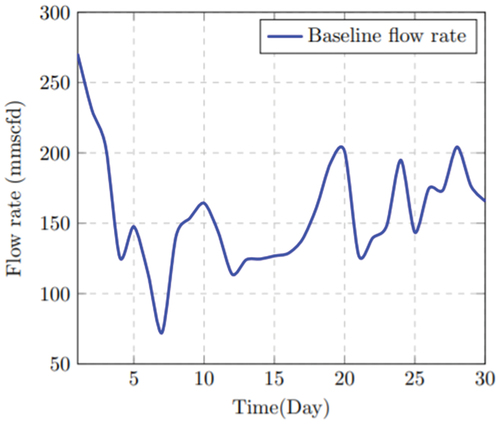
Data obtained is used to compute the baseline flow rate where monthly shortages were identified. In the BS, the mean flow rate at the beginning of the planning horizon provides a reference point to assess and compare the other scenarios.

Steady state

In a steady state, the values representing the gas flow of the system are independent of time. The computation is made in a deterministic environment where all parameters, constraints, and objective function are known. As such, the performance of the supply chain under the steady state (with no pressure variation with time) including the redundancy component can be determined.

Scenario 0: Baseline scenario

Under the baseline scenario, the mean flow rate is displayed in Figure 3. The mean flow rate amounts to 200.38 mmscfd, which means that the target mean flow of 360 mmscfd is not achieved and there is a shortfall of 159.62 mmscfd. To optimize the supply chain, the topology redundancy is introduced as a mitigation strategy in Scenario 1.

Figure 3. Baseline flow rate during the planning horizon (in days).

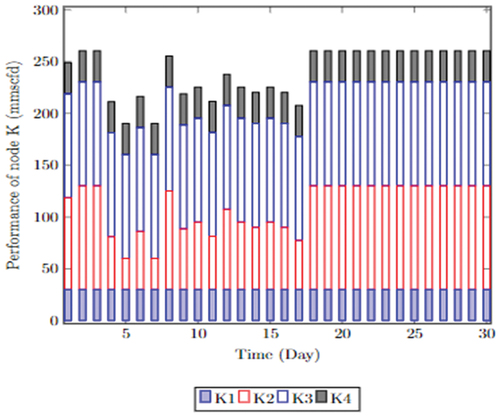
The performance level of each compressor, $\mathit{k}$, with respect to the corresponding minimum mass flow rate when ${\mathit{X}}_{\left(\mathit{k}\mathbf{,}\mathit{t}\right)}=1$ and ${\mathit{Y}}_{\left(\mathit{k}\mathbf{,}\mathit{t}\right)}=1$ is displayed in Figure 4. This is calculated by multiplying the minimum mass flow rate with the operating time of the compressor. Improved performance of the compressors is seen toward the end of the planning horizon with $\mathit{k}2$ and $\mathit{k}3,$ outperforming $\mathit{k}1$, $\mathit{k}4$.

Figure 4. Performance level of compressor k with respect to the mass flow rate under the baseline scenario (Scenario 0).

Scenario 1: Shutdown with redundancy

This scenario describes the plant shutdown with redundancy, and it operates when the disruption binary ($R_{\left(k,t\right)}=1)$ is activated. The main pipeline node closes and the trapped gas between the inlet and outlet nodes flows through the alternative pathway. Figures 5 and label Figure 6. label display the throughputs (flow rates) following the occurrence of a disruption at the specific times in the planning horizon with the presence of the relief pipeline.

Figure 5. Flow rate with no pressure drop at fixed mass flow rate.

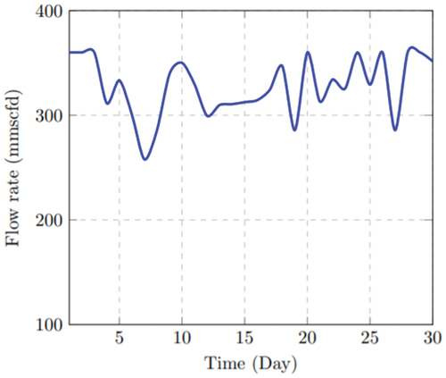
Figure 6. Flow rate with no pressure drop at varying mass flow rates.

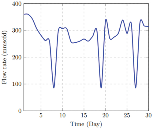
illustrates the gas flow rates for a standard mass flow rate in node $k$, while in Figure 6, the throughput reflects a varying mass flow rate introduced in node $k$ to allow the adjustment of the flow to the disruption. For the latter case, the mean flow rate is increased from 200.38 (BS) to 327.67 mmscfd.

The outputs illustrated in the graphs correspond to the flow rates with no pressure drop with time between the inlet and outlet nodes of the pipeline. Each node in the network is bound within lower and upper pressure limits. The mass balance constraint is applied to all relevant parameters, subtracting the emission losses resulting from the compressor plant shutdown. The improved flow rate is obtained by relaxing the disruption period such that the shutdown time is defined. The shutdown of the compressor station means that at least one compressor plant among $k1$ to $k4$ in the mainline is not operating during the entire shutdown period. To achieve the results in Figures 5 and label Figure 6. label, node $k2$ must be operating at the start of the planning horizon, such that the scheduling of supply to consumers comes from one to two compressors at any given time.

The performance level (throughput) of each node $k$ is illustrated in Figure 7, where there is gas flow from the mainline to the relief pipe during the shutdown at time t $\left(R\mathrm{\_}{F}_{\left(k,z,t\right)}=1\right)$, and when $X_{\left(k,t\right)}=0$ and $Y_{\left(k,t\right)}=1$. To assess the performance of the node ($k1$ to $k4$), the minimum mass flow rates is multiplied by the operating time of the compressor. While $k3$ and $k4$ remained unchanged, the performance of $k1$ increased and $k2$ varied in relation to the baseline scenario.

Figure 7. Performance level of the compressor mass flow rate when the plant starts operating after a shutdown (Scenario 1).

Scenario 2: Flow Constraint in Extended Time

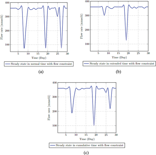
In scenario 2, the upper and lower bound flow constraints (34) and (35), are introduced. The flow constraint introduces the upper and lower bound of the flow before and during the shutdown to ensure the total flow entering the inlet node and the total flow leaving the outlet node are within bound limits. This scenario is a combination of extended time sequence at successively equally spaced points and flow constraints when the redundancy is operating. To capture all possible changes that may affect the throughput, the input series is extended twice the original length to the end of the corresponding period by halving the number of each time steps throughout the planning horizon.

The extended time-series is introduced where the impact of the flow constraint on the throughput is investigated such that the flow from the processing plant to the compressor is subject to the min/max mass flow rate of the operating status of the plant. Additional operating time of the plant does not affect all the compressors at the same time. As displayed in Figure 8(a), the only exceptions are the shutdown times of $t8$, $t19$ and $t27$. For the normal period (Figure 8(b)), the no operating time is at $t9$ where only $k3$ is affected, while for the extended time (Figure 8(c)), the no operating time is found at t8.5 where $k3$ is not operating, and $t19.5$ where $k1,k2$ and $k3$ are not operating. The average throughput resulting under Scenario 2 conditions amounts to 336.078 mmscfd.

Figure 8. Steady state with flow constraint (Scenario 2).

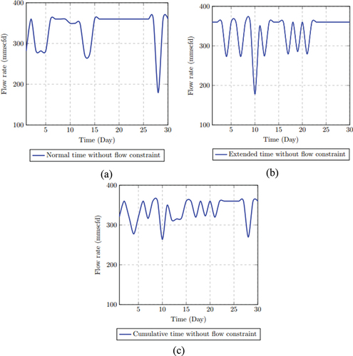
Scenario 3: No Flow Constraint in Extended Time

Scenario 3 is introduced to evaluate the impact on the overall system performance when the flow constraint is removed from the optimization problem. The extended time-series is also introduced without a corresponding upper and lower bound flow constraint. The flow rate performance for normal, extended and cumulative time in this scenario is shown in Figure 9(a-c). The defined shutdown times (undefined, undefined, and undefined) performed at optimal which is seen in the average throughput. In fact, the average throughput improved from 336.078 mmscfd (with the flow constraint) to 336.900 mmscfd (without the flow constraint).

Figure 9. Flow rate without flow constraint in extended time (Scenario 3).

Transient state

The transient effects of time-varying demand for natural gas affect the compressor and pipeline operations mainly just ahead of the delivery point. Studying the transient condition is restricted to the mainline transmission node with an extended observation time until the opening of the relief valve. The mainline closure during the disruption produces a pressure buildup. The gas accumulation suggests an expected pressure rise with time after the closure at these nodes. The gas compressibility allows for continuous pumping of gas from the upstream over a period, which eventually increases the line pack in the midstream and downstream echelons.

Scenario 4: Pressure surge from plant closure

In scenario 3, the transient state is investigated during a cumulated period of 24hrs. Each hour is divided into 6-min intervals, making a total of 10 points for every hour. The operating status of the plant node between the gas plant and the compressor is multiplied by the binary variable $\left(X_{\left(k,t\right)}\right)$ for operation on lower and upper bounds of the flow to determine the variation. The pressure interaction in the outlet node is determined by multiplying the binary variable $\left(R_{\left(k,t\right)}\right)$ with the maximum pressure upper and lower bound limit of the disruption in the mainline.

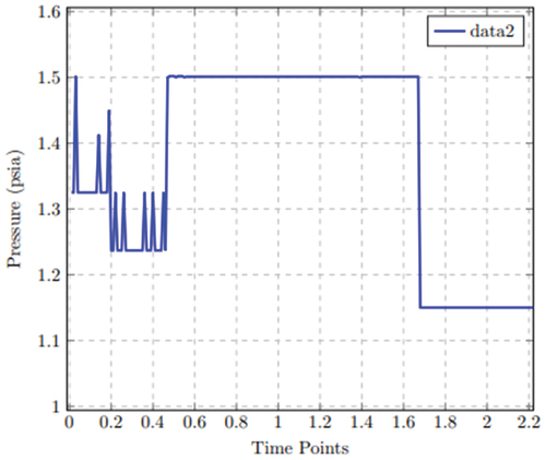
Figure 10 shows the mainline pressure variation time series at maximum mass flow rate. In Figure 11, the mainline pressure variation with time is determined using the minimum mass flow rate. During the shutdown, the pressure time-series in the mainline in both cases rises to maximum pressure between time points 0.48 to 1.67 at approximately 13:50 hrs before dropping to a stable pressure rate of 0.765 and 1.15 psia, respectively, from point 168 to 222 at approximately 10:00 hrs.

Figure 10. Pressure variation when mass flow rate is maximum.

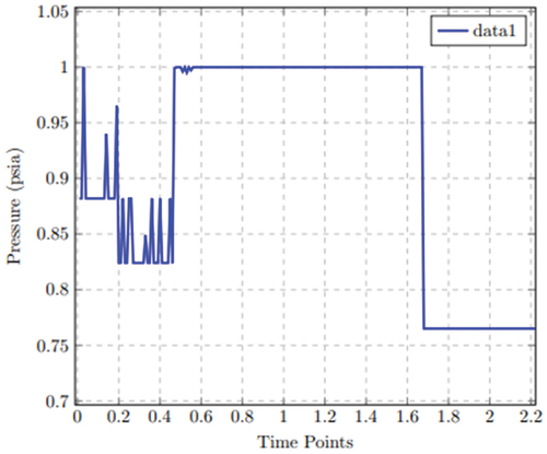
Figure 11. Pressure variation when mass flow rate is minimum.

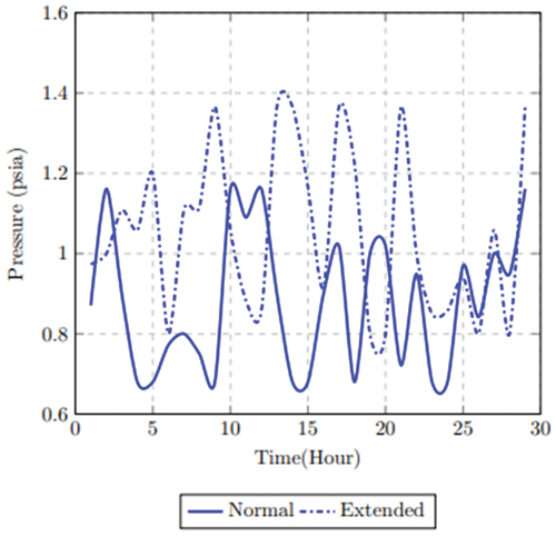
Also, the pressure interaction is examined when the alternative pathway is operating. Ignoring the bound limit of the inlet and outlet pressure while introducing the mass flow rate for the alternative pathway, the time-series at the point of variation is separated between the normal and extended time to examine the pressure interaction. As shown in Figure 12, there is close interaction between the pressure variation in both the normal and extended times displayed when the compressibility factor equals 1. This means that the deviation of the real gas from the ideal gas is insignificant and therefore does not affect the throughput in the alternative pathway. If the compressibility factor is less than 1 (z < 1), the pressure interaction in the redundancy is then shown in Figure 13. A reduced mass flow rate from 400 mmscfd in the mainline to 120 mmscfd in the relief pipe during the plant shutdown without changing the originating pressure will cause a pressure rise, which will be compensated as the gas enters the sale line. At this point, the relief pipe and the sale line are operating simultaneously.

Figure 12. Outlet pressure interaction when compressibility factor equals 1.

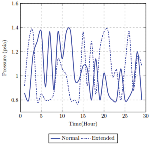
Figure 13. Outlet pressure when compressibility factor is lower than 1.

Scenario 5: Prolonged inlet and outlet nodes closure

Scenario 4 explains the unsteady condition caused by prolonged closure of both the inlet and outlet nodes on the mainline. If the closure of the nodes is within an allowable time based on the pipeline interim storage capacity, the gas will continue to flow from the upstream, which is temporarily stored until the inlet and outlet nodes are opened. On the contrary, if the disruption period on node k exceeds the projected allowable time, then the accumulated gas is emitted because of continuous pressure rise. The pressure behavior is examined over a 24hrs period at 6 mins intervals in the mainline and the relief pipeline represented as inlet and outlet nodes. The pressure in the mainline also known as the inlet pressure as shown in Table 3 starts to increase at approximately 11:54hrs triggering the outlet pressure to decrease once the alternative pathway is opened. At the point when the control valve in the alternative pathway is opened, the outlet pressure is relatively stable but changes slightly over time. The variation becomes more evident over time as gas continues to enter the alternative pathway. The pressure then normalizes as gas is fed into the sale line from the alternative pathway. Assuming the mainline inlet valve is re-opened, pressure begins to increase at approximately 17:48 hrs, which is offset as the gas begins to flow into the relief line.

Table 3. Pressure activity in Mainline during disruption.

Description	Performance	Pressure (psi)	Behavior
Mainline pipe node when the valve is closed at inlet node.	Increased at 11:54	1389	Stable
	Decreased at 17:48	1316	Stable
	Decreased at 23:42	1276	Stable
Opening of the relief valve and re-opening of mainline valve.	Decreased at 11:54	1260	Stable
	Increased at 17:48	1330	Stable
	Increased at 23:42	1375	Stable

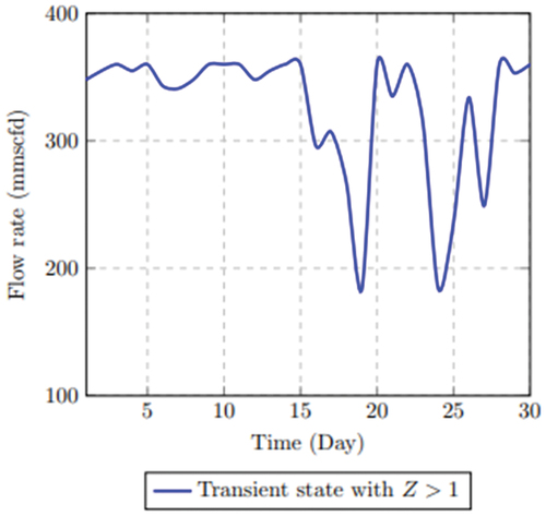
The flow rate when the relief valve is opened (operating alternative pathway) and when the compression factor equals 1 with extended time is shown in Figure 14. This indicates that the effect of the shutdown is minimized. The optimized flow rate in Figure 15 is obtained when the pressure bound limit is introduced. The impact of the pressure change on the flow rate is given as 321.17 mmscfd, which corresponds to an improved flow rate. In Figure 15, the pressure bound limit is also introduced but the compression factor is larger than 1 resulting in a flow rate output of 327.03 mmscfd.

Figure 14. Pressure bound limit in extended time.

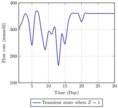
Figure 15. Pressure bound limits, higher compressibility factor in extended time.

In Table 4, the results from all scenarios in both steady and transient states are presented. The best optimal result in comparison to alternatives is compared across all feasible alternatives.

Table 4. Comparison of throughput across different cases.

State	Description	Throughput (mmscfd)
Steady	Optimized flow obtained if the capacity of node k is the same for all period in the planning horizon.	327.67
	Optimized flow is obtained if the capacity of node k varies at different rates in the planning horizon.	276.38
	Optimized flow is obtained when the flow constraint is introduced.	336.078
	Optimized flow is obtained when the flow constraint is removed.	336.90
Transient	Pressure variation in extended time.	200.38
	When compression factor equals 1 with an extended time.	321.17
	When pressure bound limit is introduced in extended time.	323.37
	The compression factor is increased in extended time.	327.03

The throughput performance of the system improved by over 63% when comparing scenario 5 to the baseline throughput performance of 200.38 mmscfd. Moreover, 93.6% of the target throughput performance of 360 mmscfd has been achieved when considering scenario 3. The best optimal solution was found in the steady state scenarios, when the flow constraint is removed.

Concluding remarks and discussion

A novel MILP model has been presented to study the impact of a proposed workflow on a natural gas supply chain when interrupted. The proposed optimization framework investigates both steady and transient state scenarios, taking into consideration relevant constraints. The system’s interruption is introduced at specified time instances and the relief pipe is activated when the inlet and outlet mainline nodes are closed. The relief pipe serves as an alternative pathway to mitigate the disturbance. The results have shown an improvement to the resilience of case study NG supply chain, following the introduction of the contingency. More in specific, the performance of the system was improved achieving an additional throughput of 127.29 mmscfd with no pressure drops when the contingency pipeline was introduced. An even better performance was obtained with the introduction of the flow constraint (Scenario 2) with a throughput of 336.078 mmscfd and a slight improvement of 336.900 mmscfd when Figure 15 time-series data is extended, and the flow constraint is removed (Scenario 3).

In the transient state, findings show that as the downstream pressure is reduced, the flow rate will increase to keep the upstream pressure constant. The additional pathway can remain open even after the mainline valves are re-opened, providing a two-way simultaneous flow to compensate for shortages pending when supply is improved. The increased compression factor in the extended time produced a flow rate of 327.03 mmscfd, which is an optimal solution in the transient state.

The developed model can be adopted in other supply chain systems after appropriate modifications are introduced based on the peculiarity of the system under review. Although the case study uses a relatively simple pipeline network, the model is versatile and able to simulate more complex problems with a larger number of nodes and pipes (e.g., system process integration) by exhibiting global optimum with well-defined solutions. The deployment of the alternative route for gas flow during the plant’s shutdown results in economic cost implication, which has not been considered in this work. To the best of the authors’ knowledge, this is the first work that addresses the optimization of the NG supply chain focusing on resilience aspects and in specific the optimization of throughput and emission losses, while considering an additional redundancy pipeline design aiming at mitigating the disruption effects. This research can be further developed to introduce more scenarios and perform a cost-benefit and lifecycle analysis to assess the cost implication compared to environmental and economic benefits.

Future studies in this area could further investigate the following aspects:

• Identification of the most suitable location to introduce the redundancy depending on the network’s need over the planning horizon to satisfy demand and loss reduction is a critical issue, as a wrong location may induce significant challenges.

• Further research optimization modeling should consider savings on downtime and how downtime minimization will lead to profit maximization for the system operators.

• A similar study could be carried out in a stochastic environment where logical consideration of uncertainty can help estimate future expectations, calculate likely returns, and estimate associated risks.

Nomenclature

Indices/Sets

I	=	Set of all suppliers, $i\in I$
$J$	=	Set of processing plant producers, $j\in J$
$K$	=	Set of compressors, $k\in K$
$G$	=	Set of city gate stations, $g\in G$
$M$	=	Set of power plant consumers, $m\in M$
$W$	=	Set of gas storage stations, $w\in W$
$Q$	=	Set of industrial consumers, $q\in Q$
$T$	=	Set of time periods, $t\in T$
$P$	=	Set of pipelines, $p\in P$
$Z$	=	Set of relief pipelines, $z\in Z$
$N$	=	Set of domestic/commercial consumers, $n\in N$

Parameters

$\alpha u_{(p)}$	=	Pressure of pipeline, p, at the start
${\mathrm{\Delta }}_{(\mathrm{k})}$	=	Number of shutdowns at compressor plant, k
$h_{\left(j\right)}^{max}$	=	Maximum mass flow rate of processing plant, j
$h_{\left(j\right)}^{min}$	=	Minimum mass flow rate of processing plant, j
$c{p}_{\left(k,t\right)}^{min}$	=	Maximum compressor capacity, k, at time, t
$d\mathrm{\_}{a}_{\left(m,t\right)}$	=	Demand capacity for consumer, m, at time, t
$d\mathrm{\_}{b}_{\left(n,t\right)}$	=	Demand capacity for consumer, n, at time, t
$d\mathrm{\_}{c}_{\left(q,t\right)}$	=	Demand capacity for consumer, q, at time, $t$
$emissio{n}_{(k,t)}$	=	Loss through emission at compressor, k, during the shutdown at time, $t$
$g_{\left(i\right)}^{min}$	=	Maximum mass flow rate from all gas suppliers, i
$In{c}_{(p,t)}$	=	Capacity of pipeline, p, before expansion at time, $t$
$j{c}_{\left(i,t\right)}^{max}$	=	Maximum processing plant capacity of supplier, i, at time, t
$m{c}_{\left(k\right)}^{max}$	=	Maximum pressure in the compressor, $k$
$m{c}_{\left(k\right)}^{min}$	=	Minimum pressure in the compressor, $k$
${\mathrm{O}}_{\left(k\right)}$	=	Maximum offline time after the shutdown of compressor, $k$
$ph{i}_{\left(g,t\right)}^{max}$	=	Maximum city gate capacity, g, at time, t
$P{C}_{\left(p\right)}^{max}$	=	Maximum pressure into pipeline,$p$
$P{C}_{\left(p\right)}^{min}$	=	Minimum pressure into pipeline,$p$
$r{c}_{\left(m,t\right)}^{max}$	=	Maximum capacity of power plant, m, at time, $t$
$r{p}_{\left(z,t\right)}^{max}$	=	Maximum relief pipe capacity, z, at time, $t$
$s_{\left(k\right)}^{max}$	=	Maximum mass flow rate of compressor, $k$
$s_{\left(k\right)}^{min}$	=	Minimum mass flow rate from compressor, $k$
$s{c}_{\left(i,t\right)}^{max}$	=	Maximum supply gas fields capacity, i, at time, $t$
$s{t}_{\left(w,t\right)}^{min}$	=	Minimum storage capacity, w, at time, $t$
$s{t}_{\left(w,t\right)}^{max}$	=	Maximum storage capacity, w, at time, $t$
$y{s}_{\left(w,t\right)}$	=	Initial inventory level, w, at time, $t$
$v_{\left(z\right)}^{max}$	=	Maximum mass flow during the shutdown in relief pipeline, z
$v_{\left(z\right)}^{min}$	=	Minimum mass flow during the shutdown in relief pipeline, z
$Z{h}_{\left(z\right)}^{min}$	=	Minimum pressure bound of relief pipeline, z, during operation
$Z{h}_{\left(z\right)}^{max}$	=	Maximum pressure bound of relief pipeline, z, during operation
$\gamma Z_{\left(p\right)}$	=	Pipeline temperature at the start and end nodes of pipeline,$p$
${\delta }_{\left(k\right)}$	=	Minimum offline time of compressor, $k$
$\delta P_{\left(t\right)}$	=	Total number of periods that plants have been shutdown at time, t
$\delta Z_{\left(k\right)}$	=	The initial state of the plant with respect to the total period that plant node, $k$, has been continuously shutdown
${\epsilon }_{\left(k\right)}$	=	Compressor factor in compressor node, $k$
$\theta P_{\left(p\right)}^{max}$	=	Maximum proportional capacity for expansion of pipeline,$p$
$\theta P_{\left(p\right)}^{min}$	=	Minimum proportional capacity for expansion of pipeline,$p$
$\lambda Z_{\left(p\right)}$	=	Pipeline diameter of pipeline,$p$
$\mathrm{\Psi }{P}_{\left(k\right)}$	=	The operation period after the startup of plant, $k$
${\mathrm{\Psi }}_{\left(k\right)}$	=	Minimum online time after the startup of compressor plant, $k$

Decision Variables

$B\mathrm{\_}{S}_{\left(w,t\right)}$	=	Level of gas storage, w, at time,
$L\mathrm{\_}{T}_{\left(k,t\right)}$	=	Monthly loss target at compressor node, $k$, at time, $t$
$P_{\left(j,k,t\right)}^{in}$	=	Pressure inlet from node, $j$, to compressor node, $k$, at time, $t$
$P_{\left(j,k,t\right)}^{out}$	=	Pressure outlet from node, $j$, to compressor node, $k$, at time, $t$
$P_{\left(k,z,t\right)}^{out}$	=	Pressure outlet from compressor node $k$, to relief node, z, at time, $t$
$P_{\left(p\right)}^{in}$	=	Pressure in the inlet node of pipeline,$p$
$P_{\left(p\right)}^{out}$	=	Pressure in the outlet node of pipeline,$p$
$P_{\left(z\right)}^{Bar}$	=	Pressure in the relief pipe node, z
$S\mathrm{\_}{T}_{\left(k,m,t\right)}$	=	Gas shortage volume from compressor node, $k$, to node, $m$, at time, $t$
$X\mathrm{\_}{P}_{\left(j,k,t\right)}$	=	Gas volume transmitted from processing node $j$to compressor node, $k$, at time, $t$
$Y\mathrm{\_}{F}_{\left(k,g,t\right)}$	=	Gas volume transmitted from compressor node, $k$, to node, $g$, at time,$t$
$Y\mathrm{\_}{W}_{\left(k,m,t\right)}$	=	Gas volume transmitted from compressor node $k$, to consumer, $m,$at time, $t$
$Y{C}_{\left(g,q,t\right)}$	=	Gas volume distributed from city gate node, $g,$ to consumer, $q,$ at time$,t$
$Y{M}_{\left(w,k,t\right)}^{-}$	=	Gas volume from storage inventory, w, to compressor station, k, at time, $t$
$Y{M}_{\left(k,w,t\right)}^{+}$	=	Gas volume transmitted from compressor node, $k$, to gas storage,$w$, at time, $t$
$Y{P}_{\left(g,n,t\right)}$	=	Gas volume distributed from city gate station node, $g$, to consumer, $n,$at time, $t$
$Z_{\left(t\right)}^E$	=	Total amount of losses at time, $t$
$Z{A}_{\left(i,j,t\right)}$	=	Gas volume transmitted from node, $i,$ to processing plant, $j,$ at time, $t$
${\delta }_{\left(z,t\right)}^{inc}$	=	Capacity increment of relief pipeline, $z,$ at time, $t$

Binary Variables

$H_{\left(z,t\right)}$	=	= 0, if redundancy is not activated at time, $t$; otherwise, 1
$P{I}_{\left(j,k\right)}$	=	= 1, if there is gas flow from node, j, to compressor node, k; otherwise, 0
$P{I}_{\left(k,z\right)}^{-}$	=	= 1, if there is gas flow from compressor node, k, to node, z; otherwise, 0
$R_{\left(k,t\right)}$	=	= 0, if compressor node, $k$, operates at time, $t$; otherwise, 1
$R\mathrm{\_}{F}_{\left(k,z,t\right)}$	=	=1, if there is gas flow from compressor node, k, to relief pipe, $z$, during the shutdown at time, $t$; otherwise, 0
$X_{\left(k,t\right)}$	=	= 0, if there is no start up for compressor node, $k$, at the beginning; otherwise, 1
$Y_{\left(k,t\right)}$	=	= 1, if compressor node, $k$, shuts down at time, $t$; otherwise, 0

Acknowledgement

The authors would like to acknowledge the Petroleum Technology Development Fund (PTDF), for the financial sponsorship throughout the realization of this work.

Disclosure statement

No potential conflict of interest was reported by the author(s).

Additional information

Funding

The work was supported by the Petroleum Technology Development Fund .

References

- Abahussain, M. M., and R. D. Christie. 2013. Optimal scheduling of a natural gas processing facility with price-based demand response. In IEEE Power and Energy Society General Meeting. doi:10.1109/PESMG.2013.6672280.
- Alves, F. D. S., J. N. M. de Souza, and A. Luiz Hemerly Costa. 2016. Multi-Objective design optimization of natural gas transmission networks. Computers & Chemical Engineering 93:212–26. doi:10.1016/j.compchemeng.2016.06.006.
- Balcombe, P. B., N. P. Hawkes, and A. D. 2018. Characterising the distribution of methane and carbon dioxide emissions from the natural gas supply Chain. Journal of Cleaner Production 172:2019–32. doi:10.1016/j.jclepro.2017.11.223.
- Bopp, A. E., R. K. Vijay, S. W. Palocsay, and S. P. Stevens. 1996. An Optimization model for planning natural gas purchases, transportation, storage and deliverability. Omega 24 (5):511–22. doi:10.1016/0305-0483(96)00025-4.
- British petroleum. 2019. BP Energy Outlook 2019 Edition. London, UK: British Petroleum. Accessed 10 December 2020.
- British Petroleum. 2020. “BP Statistical Review of World Energy.“ 69th Edition. Accessed 30 December 2020.
- Carvalho, H., et al. 2012. “Supply Chain Redesign for Resilience Using Simulation.” Computers & Industrial Engineering 62(1): 329–41. 10.1016/j.cie.2011.10.003
- Carvalho, R., L. Buzna, F. Bono, M. Masera, D. K. Arrowsmith, and D. Helbing 2014. “Resilience of Natural Gas Networks during Conflicts, Crises and Disruptions.” Plos One. PLoS ONE 9 3 e90265 10.1371/journal.pone.0090265
- Christopher, M., and H. Peck. 2004. Building the Resilient Supply Chain. The Internaltional Journal of Logistics Management 15 (2):1–14. doi:10.1108/09574090410700275.
- Cimellaro, G. P., O. Villa, and M. Bruneau. 2015. Resilience-Based Design of Natural Gas Distribution Networks. Journal of Infrastructure Systems 21 (1). doi:10.1061/(ASCE)IS.1943-555X.0000204.
- Doukas, H., A. Flamos, and J. Psarras. 2011. Risks on the Security of Oil and Gas Supply. Energy Sources, Part B: Economics, Planning, and Policy 6 (4):417–25.
- El-Shiekh, T. M. 2013. The Optimal Design of Natural Gas Transmission Pipelines. Energy Sources, Part B: Economics, Planning, and Policy 8 (1):7–13.
- Emenike, S.N., and G. Falcone. 2020. A Review on Energy Supply Chain Resilience through Optimization. Renewable and Suatainable Energy Reviews 134: 110088. doi:10.1016/j.rser.2020.110088.
- Farzaneh-Gord, M., and H. Reza Rahbari. 2016. Unsteady Natural Gas Flow within Pipeline Network, an Analytical Approach. Journal of Natural Gas Science and Engineering 28:397–409. doi:10.1016/j.jngse.2015.12.017.
- Hamedi, M., F. Reza Zanjirani, M. H. Mohammad, and R. E. Gholam. 2009. A Distribution Planning Model for Natural Gas Supply Chain: A Case Study. Energy Policy 37 (3):799–812. doi:10.1016/j.enpol.2008.10.030.
- Hao, H., Z. Liu, F. Zhao, and W. Li. 2016. “Natural Gas as Vehicle Fuel in China: A Review.” Renewable and Sustainable Energy Reviews. Elsevier Ltd. 62 521–33 10.1016/j.rser.2016.05.015
- Hoggett, R. 2014. Technology Scale and Supply Chains in a Secure, Affordable and Low Carbon Energy Transition. Applied Energy 123:296–306. doi:10.1016/j.apenergy.2013.12.006.
- Hutagalung, A. M., D. Hartono, M. Arentsen, and J. Lovett. 2017. The Economic Implications of Natural Gas Infrastructure Investment. Energy Sources, Part B: Economics, Planning, and Policy 12 (12):1080–87.
- Ioannou, A., et al. 2019. “Multi-Stage Stochastic Optimization Framework for Power Generation System Planning Integrating Hybrid Uncertainty Modelling.” Energy Economics 80: 760–76. (September 18, 2019). 10.1016/j.eneco.2019.02.013
- Lee, Y. H., and S. Han Kim. 2002. Production–distribution Planning in Supply Chain Considering Capacity Constraints. Computers & Industrial Engineering 43 (1–2):169–90. doi:10.1016/S0360-8352(02)00063-3.
- Mac, K., M. A. Brouwer, and J. Scott Samuelsen. 2018. The Role of Natural Gas and Its Infrastructure in Mitigating Greenhouse Gas Emissions, Improving Regional Air Quality, and Renewable Resource Integration. Progress in Energy and Combustion Science 64:62–92. doi:10.1016/j.pecs.2017.10.002.
- Menon, S. E. 2005. GAS PIPELINE HYDRAULICS. First. New York: Taylor & Francis Group. Accessed 20 November 2020.
- Mikolajková, M., C. Haikarainen, H. Saxén, and F. Pettersson. 2017. Optimization of a Natural Gas Distribution Network with Potential Future Extensions. Energy 125:848–59. doi:10.1016/j.energy.2016.11.090.
- Pourhejazy, P., O.K. Kwon, Y.T. Chang, and H.K. Park. 2017. Evaluating resiliency of supply chain network: a data envelopment analysis approach. Sustainability 9 (2):255. doi:10.3390/su9020255.
- Ríos-Mercado, R. Z., and C. Borraz-Sánchez. 2015. Optimization Problems in Natural Gas Transportation Systems: A State-of-the-Art Review. Applied Energy 147:536–55. doi:10.1016/j.apenergy.2015.03.017.
- Sabri, E. H., and B. M. Beamon. 2000. A Multi-Objective Approach to Simultaneous Strategic and Operational Planning in Supply Chain Design. Omega 28 (5):581–98. doi:10.1016/S0305-0483(99)00080-8.
- Sayed, A. R., C. Wang, and T. Bi. 2019. Resilient Operational Strategies for Power Systems Considering the Interactions with Natural Gas Systems. Applied Energy 241:548–66. doi:10.1016/j.apenergy.2019.03.053.
- Sheikhnejad, Y., J. Simões, and N. Martins. 2020. Energy Harvesting by a Novel Substitution for Expansion Valves: Special Focus on City Gate Stations of High-Pressure Natural Gas Pipelines. Energies 13 (4):956.
- Shin, H., et al. 2019. “Environmental Shutdown of Coal-Fired Generators for Greenhouse Gas Reduction: A Case Study of South Korea.” Applied Energy 252. 10.1016/j.apenergy.2019.113453
- Tomasgard, A., F. Rømo, K. Midthun, and M. Fodstad. 2007. Optimization Models for the Natural Gas Value Chain. In Geometric Modelling, Numerical Simulation, and Optimization, ed. E. Quak and G. Hasle,K. Lie. Berlin, Heidelberg: Springer. pp. 521–555. doi:10.1007/978-3-540-68783-2_16.
- UNFCCC. 2015. The Paris Agreement. Paris.
- Vasconcelos, C. D., S. Ricardo Lourenço, A. Carlos Gracias, and D. Alves Cassiano. 2013. Network flows modeling applied to the natural gas pipeline in Brazil. Journal of Natural Gas Science and Engineering 14:211–24. doi:10.1016/j.jngse.2013.07.001.
- Yasser, A., K. Barker, and L. A. Albert. 2019. Resilience-driven restoration model for interdependent infrastructure networks. Reliability Engineering & System Safety 185:12–23. doi:10.1016/j.ress.2018.12.006.
- Zarei, J., and M. Reza Amin-Naseri. 2019. An integrated optimization model for natural gas supply Chain. Energy 185:1114–30. doi:10.1016/j.energy.2019.07.117.
- Zhang, B., et al. 2020. Economic and environmental co-benefit of natural gas supply chain considering the risk attitude of designers. Journal of Cleaner Production 272. 10.1016/j.jclepro.2020.122681