Uncovering the mystery of financial development in mitigating CO2 emissions in China: A spatial dependence and heterogeneity perspective

ABSTRACT

Carbon dioxide (CO₂) emission mitigation has recently been a critical policy-making concern in the financial area. To address this concern, we examine whether and to what extent financial development reduces CO₂ emissions in China from a spatial dependence and heterogeneity perspective. The empirical results of applying a random effects eigenvector spatial filtering (RE-ESF) model and a RE-ESF with non-spatially varying coefficients (RE-ESF-SNVC) model to a provincial panel dataset over the period 1997 − 2017 indicate better goodness-of-fit due to the consideration of spatial effects. The role of financial development in mitigating CO₂ emissions is confirmed at both the global level by using the RE-ESF model and the local level by using the RE-ESF-SNVC model. Moreover, the contributions of financial development display clear regional disparities, suggesting the inclusion of spatial heterogeneity when developing financial policies for CO₂ emission mitigation. However, such contributions are restricted by financial constraints which increase CO₂ emissions globally and locally, requiring a balance between financial development and financial constraints when expanding bank loans. Additionally, the one-way analysis of variance reveals the existence of a geographically dividing line approximately connecting the easternmost tip of Xinjiang and the easternmost tip of Fujian. It is observed that provinces above the line generally have stronger impacts of financial development on carbon emission reduction, while impacts in provinces below the line are generally weaker. These findings encourage the implementation of proactive fiscal and monetary policies to promote financial development. Considering financial constraints, cross-provincial and province-specific financial policies should be balanced when allocating more financial resources to provinces with greater contributions of financial development to CO₂ emission mitigation.

KEYWORDS:

• Environmental sustainability
• spatial heterogeneity
• panel data analysis
• cross-provincial collaboration
• geographically dividing line

1. Introduction

The ever-increasing amount of human-induced carbon dioxide (CO₂) emissions has imposed great challenges on the global environment and public health, and thus has become a worldwide concern. Particularly, owing largely to its reliance on fossil fuels, China has achieved remarkable growth in its gross domestic product (GDP) over the past decades along with a significant increase in CO₂ emissions. As reported in Statistical Review of World Energy (2021),¹ China’s CO₂ emissions rose from 7.7 billion tonnes in 2009 to 9.9 billion tonnes in 2020, accounting for approximately 31% of the world’s total carbon emissions in 2020. To better cope with the carbon emission concern, the Chinese government promised to “have CO₂ emissions peak before 2030 and achieve carbon neutrality before 2060” and explicitly committed a 65% drop in carbon intensity (i.e., CO₂ emissions per unit of GDP) by 2030 from the 2005 level (Chen et al. 2021; Tang, Mei, and Zou 2021). As a result, CO₂ emission mitigation has been a crucial consideration for China’s industrial policy formulation, putting China on the path to achieve its ambitious goals of “carbon peak and carbon neutrality” and a low-carbon transition economy.

In the financial area, great efforts have been devoted to investigating how financial policy-making influences CO₂ emissions with special emphasis on financial agglomeration (Yuan et al. 2019), financial support (Zhou et al. 2019), financial structure (Kim, Wu, and Lin 2020), financial development (Zhao and Yang 2020), green credit (Zhang et al. 2021), and so on. Among them, financial development has commonly been regarded as a comprehensive measurement of the depth, access, efficiency, and stability of the financial system in an economy and has gained considerable research in terms of attention to examine its impact on CO₂ emissions (Haseeb et al. 2018; Zhao and Yang 2020). Generally, financial development can influence carbon emissions in the following ways. First, a higher level of financial development usually indicates that firms are more likely to access financial resources (e.g., bank loans). This may not only increase firms’ investments in researching, manufacturing, and adopting low-carbon technologies but also expand their production activities, leading to ambiguous impacts on carbon emissions (Lahiani 2020). Second, a more advanced financial system usually provides consumers with more credit products, potentially increasing their expenditures on both high energy-consuming (e.g., automobiles) and energy-saving (e.g., solar air conditioning) products (Yang et al. 2021). Third, from a government viewpoint, a developed financial sector is more likely to increase governmental expenditures on environmental protection and education by providing firms and consumers with financial incentives to use energy-conserving or environmentally friendly technologies and products (Yuan et al. 2018). However, it may also promote foreign direct investment (FDI) and expand local production and trade activities, potentially generating more carbon emissions.

In reality, the above three ways of capturing the impact of financial development on CO₂ emissions work together and yield an inconclusive result. This motivates us to reexamine whether and to what extent financial development reduces CO₂ emissions in China. To this end, this paper takes a spatial dependence and heterogeneity perspective that has not received sufficient attention previously and employs a random effects eigenvector spatial filtering (RE-ESF) model and a RE-ESF with non-spatially varying coefficients (RE-ESF-SNVC) model to a provincial panel dataset over the period 1997 − 2017 (Lv and Li 2021; You and Lv 2018; Zhao and Yang 2020). In so doing, this paper can contribute to the existing studies in the following two aspects. First, compared to the commonly used global spatial models (e.g., spatial lag model, spatial error model, spatial Durbin model), the RE-ESF and RE-ESF-SNVC models demonstrate advantages in capturing both the global and the local relationships between factors and carbon emissions (Yu et al. 2020). This enables policy-makers to consider spatial heterogeneity and shift from a one-size-fits-all approach to province-specific financial policy-making for CO₂ emission mitigation. Second, this paper enriches the existing research by confirming a clear “northeast‒southwest” spatial pattern of the impact of financial development on carbon emission reduction that can be approximated by a geographically dividing line connecting the easternmost tip of Xinjiang and the easternmost tip of Fujian.

The remainder of this paper is structured as follows. Section 2 reviews previous findings regarding how financial development influences carbon emissions. Section 3 describes the identified factors, spatial characteristics of CO₂ emissions and the RE-ESF approach. Section 4 reports the empirical results with respect to the pooled panel model, the RE-ESF and RE-ESF-SNVC models, and the geographically dividing line. Section 5 presents discussions and implications, and Section 6 concludes this paper.

2. Literature review

2.1. Financial development and CO₂ emissions

A large number of studies have provided evidence supporting that financial development can mitigate CO₂ emissions. For example, using BRIC economies’ panel data over the period 1992–2004, Tamazian, Chousa, and Vadlamannati (2009) argue that a higher degree of financial development tends to decrease environmental degradation with a special emphasis on the role of financial liberalization and openness in reducing CO₂ emissions. Within the cointegration framework, Jalil and Feridun (2011) identify income, energy consumption and trade openness as the main determinants of CO₂ emissions in China over 1953–2006 and conclude that financial development has led to a decrease in environmental pollution. By measuring financial development as domestic credit to the private sector as a share of GDP, Dogan and Seker (2016) find that an increase in financial development tends to decrease CO₂ emissions in the top renewable energy countries over 1985–2011. Zhao and Yang (2020) construct a provincial financial development index for China over 2001–2015 and confirm the presence of regional disparities regarding how financial development mitigates CO₂ emissions. As suggested by the static panel analysis, financial development will reduce emissions in all provinces except for Zhejiang, Fujian, Sichuan, Yunnan, Shaanxi, and Xinjiang, while the dynamic panel analysis indicates significantly lagging inhibitory effects of financial development on emissions. Taking a spatial perspective and using panel data from 97 countries over 2000–2014, Lv and Li (2021) provide evidence supporting that countries with higher levels of local and neighboring financial development can significantly reduce CO₂ emissions. Using bank credit indicators as a proxy for financial development, Liu and Gong (2022) consider the spatial-temporal heterogeneity and conclude that financial development inhibits carbon emissions in most provinces most of the time. In addition, the role of financial development in mitigating CO₂ emissions is also confirmed in Shahbaz et al. (2013) for Malaysian economy over 1971–2011, Shahbaz et al. (2013) for Indonesian economy over 1975–2011, Shahbaz, Tiwari, and Nasir (2013) for South African economy over 1965–2008, Salahuddin, Gow, and Ozturk (2015) for Gulf Cooperation Council Countries over 1980–2012, Abbasi and Riaz (2016) for Pakistan over 1988–2011, Saidi and Mbarek (2017) for 19 emerging economies over 1990–2013, Zaidi et al. (2019) for Asia Pacific Economic Cooperation countries over 1990–2016, and Xiong et al. (2023) for China over 1997–2011.

Nevertheless, contrary findings have been widely reported in previous studies. As noted in Zhang (2011), financial development in terms of financial intermediation scale and efficiency and stock market scale and efficiency is an important driver for increasing CO₂ emissions in China over the period 1994–2009. It is also found that financial development has taken place at the expense of increasing CO₂ emissions in Farhani and Ozturk (2015) for Tunisia over 1971–2012 and in Javid and Sharif (2016) for Pakistan over 1972–2013. From a long-run perspective, a positive relationship between financial development and CO₂ emissions has been discovered in Ahmad et al. (2018) by using evidence from China over 1980–2014 and Bayar, Maxim, and Maxim (2020) through examining 11 post-transition European economies over 1995–2017. Similarly, the accelerative role of financial development in increasing CO₂ emissions and causing the degradation of the environment is also confirmed in Yazdi and Beygi (2018) for 25 African countries over 1985–2015, Moghadam and Dehbashi (2018) for Iran over 1970–2011, Salahuddin et al. (2018) for Kuwait over 1980–2013, Haseeb et al. (2018) for BRICS countries over 1995–2014, Pata (2018) for Turkey over 1974–2014, Ali et al. (2019) for Nigeria over 1971–2010, and Nasir, Huynh, and Tram (2019) for the selected ASEAN-5 economies over 1982–2014.

Apart from the above contradictory findings, there is a large body of literature reporting mixed results regarding how financial development affects CO₂ emissions. For example, an insignificant carbon effect of financial development is found in the long-run in Ozturk and Acaravci (2013) by analyzing evidence from Turkey over 1960–2007. Using panel data of 12 MENA countries over 1990–2011, Omri et al. (2015) find that the impact of financial development, represented by domestic credit to private sector as share of GDP, on CO₂ emissions is positive for Qatar, while it is negative for Jordan and insignificant for Algeria, Bahrain, Egypt, Iran, Kuwait, Morocco, Oman, Saudi Arabia, Syria, Tunisia. Nasreen and Anwar (2015) documented that the environmental impact of financial development depends on a country’s income level, demonstrating a negative impact on per capita CO₂ emissions in high-income countries but a positive carbon impact in middle- and low-income countries over 1980–2020. By comparing the results of the subperiod sample over 1988–2011 and the full sample over 1971–2011, Abbasi and Riaz (2016) conclude that financial development can reduce CO₂ emissions only in the subperiod sample with a greater degree of liberalization and financial sector development in Pakistan. Using evidence from advanced and developing countries over 1989–2013, Kim, Wu, and Lin (2020) state that a more market-led financial system tends to mitigate but eventually aggravate CO₂ emissions, while opposite carbon impacts are found for a bank-led financial system. Zhao and Yang (2020) discover that at the national level a 4%-5% decrease in carbon emissions is usually observed due to a 1% increase in the provincial financial development level. Nevertheless, at the provincial level, carbon emissions in Zhejiang, Fujian, Sichuan, Yunnan, Shaanxi and Xinjiang can be increased.

2.2. Research models

The above inconclusive findings regarding how financial development affects CO₂ emissions have been obtained from the following perspectives. First, the most common way is to investigate the causal and cointegrated relationships between financial development and CO₂ emissions by applying various causality and cointegration tests. For example, using the panel cointegration technique, Nasreen and Anwar (2015) provide evidence supporting the presence of cointegration between financial development and CO₂ emissions in high-, middle- and low-income countries. Due to its advantage in dealing with potential structural breaks in data, the autoregressive distributed lag (ARDL) bounds test has been widely employed for testing cointegration between financial development and CO₂ emissions in Farhani and Ozturk (2015) for Tunisia, Salahuddin et al. (2018) for Kuwait, Moghadam and Dehbashi (2018) for Iran, and Ali et al. (2019) for Nigeria. The causality and cointegration between financial development and CO₂ emissions have also been confirmed in Yazdi and Beygi (2018) by adopting the pooled mean group approach and Granger causality and Haseeb et al. (2018) and Bayar, Maxim, and Maxim (2020) by using Dumitrescu-Hurlin Granger causality and Westerlund cointegration tests.

Second, after confirming the cointegration between financial development and CO₂ emissions, a further issue is to capture their long-run equilibrium and short-run volatility relationships by employing a vector error correction model (VECM) or ECM. For example, using VECM and variance decomposition techniques, Zhang (2011) assesses the impacts of different financial development indicators (i.e., financial intermediation scale and efficiency, stock market scale and efficiency, foreign direct investment) on CO₂ emissions and identifies financial intermediation scale as the most important emission factor for China over 1994–2009. Many other studies have been dedicated to this issue, including Salahuddin, Gow, and Ozturk (2015), Abbasi and Riaz (2016), Javid and Sharif (2016), Pata (2018), Salahuddin et al. (2018), and Zhao and Yang (2020).

Third, the asymmetric impact of financial development on CO₂ emissions has been previously examined by using a nonlinear ARDL (NARDL) model. For example, Ahmad et al. (2018) find no evidence in support of an asymmetric relationship, indicating that positive and negative shocks to financial development demonstrate symmetric impacts on CO₂ emissions in China over 1980–2014. Using evidence from India over 1980–2014, Neog and Yadava (2020) argue that financial development positively affects CO₂ emissions but becomes statistically insignificant. Ahmed et al. (2020) note that a positive shock to financial development generates a greater impact on carbon emissions in Pakistan over 1996–2018.

Regarding the spatial impact of financial development on carbon emissions, few studies have made efforts. For example, Lv and Li (2021) employ a spatial Durbin model (SDM) with fixed effects to investigate the role of financial development in reducing carbon emissions among 97 countries over 2000–2014. As found, a country’s carbon emissions can be reduced by not only its own high financial development but also its neighboring countries with a high financial development due to the existence of significantly negative spillover effects. Using fixed effects models and instrumental variable methods for a panel dataset consisting of 285 Chinese prefecture-level cities over 2003–2016, Zhou and Zhang (2023) argue that financial deepening, financial interrelation ratio, and financial intermediary can increase carbon emissions at the national level, but the role of financial development in achieving carbon neutrality exists only in middle and western cities. In addition, a variety of econometric models have been employed to quantify the relationship between financial development and CO₂ emissions. For example, a dynamic seemingly unrelated regression is applied in Haseeb et al. (2018) for BRICS countries over 1995–2014; the dynamic ordinary least squares (DOLS) and fully modified least squares (FMOLS) are adopted in Dogan and Seker (2016) for the top renewable energy countries over 1985–2011, Nasir, Huynh, and Tram (2019) for the selected ASEAN-5 economies over 1982–2014, and Zhao and Yang (2020) for China over 2001–2015; the FMOLS and cointegrating regression (CCR) are employed in Pata (2018) for Turkey over 1974–2014; and the geographical and temporal weighted regression (GTWR) model is utilized in Liu and Gong (2022) for China over 2003–2017.

As noted earlier, financial development can influence CO₂ emissions through influencing the behavior of producers, consumers, and the government, leading to an inconclusive result. Meanwhile, the above literature review indicates that previous studies have focused mainly on the causal, cointegrated, long-run equilibrium and short-run volatility, and asymmetric relationships between financial development and carbon emissions, paying insufficient attention to their spatial dependence and heterogeneity. To overcome this weakness, this paper applies the RE-ESF and RE-ESF-SNVC models to investigate their global and local relationships, providing further spatial evidence reexamining how financial development influences CO₂ emissions from a spatial dependence and heterogeneity perspective. On the other hand, few studies take into account the scarcity of financial resources that may restrict the inhibitory effect of financial development on carbon emissions. To fill this gap, this paper incorporates financial constraints measured by the ratio of bank loans to bank deposits into empirical models and provides new empirical evidence.

3. Variables, data sources and methodology

In this section, we first identify economic factors of CO₂ emissions under the STIRPAT framework with particular attention to financial development. Then, using a Chinese provincial dataset, we detect the presence of potential spatial effects in CO₂ emissions. To deal with the detected spatial effects, we finally introduce the RE-ESF and RE-ESF-SNVC models to examine how financial development mitigates CO₂ emissions at the global and local levels.

3.1. STIRPAT framework and factor identification

As noted earlier, financial development (fdev) can influence CO₂ emissions in multiple ways, and this is the factor of interest in this paper and has been widely measured by the ratio of the sum of bank deposits and bank loans to GDP (Guo and Hu 2020; Saidi and Mbarek 2017). The main reasons for using this measurement are as follows: First, the banking sector shows significant dominance in China’s financial system. According to the data provided by the People’s Bank of China (www.pbc.gov.cn), the proportion of the banking sector in terms of the number of legal entities and the size of assets is greater than 90%, contributing up to 60.26% of the social financing scale. Thus, bank credit has been commonly considered an important financial tool for promoting economic growth (Zhou et al. 2020). Second, as found in Rojas-Suarez and Weisbrod (1996), capital markets exhibit relatively limited impacts on financial development in economically and financially underdeveloped countries and regions where the size of capital markets and the volume of stock transactions are small. Third, China’s capital markets are not fully open, and they are highly controlled, making it difficult to fully reflect the overall strength of the financial sector (Jalil and Feridun 2011).

Meanwhile, population size (pop), economic development (pgdp) and technological progress (tec) are suggested by the STIRPAT framework and can be measured by permanent residents at the end of each year, per capita GDP and per capita patent counts granted, respectively (Dietz and Rosa 1997). Notably, the square term of per capita GDP is considered to check the existence of the environmental Kuznets curve (EKC). Due to the unique nature of the commercial banking business in China, financial constraints (loanrate) measured by the ratio of bank loans to bank deposits is identified. As needed, this ratio is commonly controlled within 75% but allows for regional disparity (Yang et al. 2021). In addition, previous studies suggest the inclusion of urbanization (urb), industrial structure (is), construction intensity (cons), trade openness (trade), vehicle population (pveh) and foreign direct investment (fdi). As a result, 11 factors of CO₂ emissions are identified and presented in Table 1. For further analysis, we collected CO₂ emissions from Carbon Emission Accounts & Datasets (CEADs; https://www.ceads.net.cn/) and a balanced panel dataset of 30 Chinese mainland provinces, autonomous regions, and municipalities² over 1997–2017 from the China Statistical Yearbooks (1998–2018) and the Almanac of China’s Finance and Banking (1998–2018). To obtain the real values of pgdp, comparable prices in 1978 are used to eliminate the inflation effect. Table 2 presents descriptive statistics of the identified factors.

Table 1. Identified economic factors of CO₂ emissions.

	Variable	Measure (unit)	References
Dependent variable	CO2 emissions ($lnC{O}_2$)	Per capita carbon emissions (kg per person)	Shan et al. (2020)
Factor of interest	Financial development ($lnfdev$)	Ratio of the sum of bank deposits and bank loans to GDP (%)	Saidi and Mbarek (2017)
Control factors	Population size ($lnpop$)	Permanent residents at the end of each year (10^4 persons)	Lantz and Feng (2006)
	Economic development ($lnpgdp$)	Per capita GDP (10^4 Yuan)	Apergis and Ozturk (2015)
	Technological progress ($lntec$)	Per capita patent counts granted (piece)	Acs, Anselin, and Varga (2002)
	Financial constraint ($lnloanrate$)	Ratio of bank loans to bank deposits (%)	Ji (2013)
	Urbanization ($lnurb$)	Ratio of urban population (%)	Saidi and Mbarek (2017)
	Industrial structure ($lnis$)	Ratio of the added value of the secondary industry to GDP (%)	Apergis and Ozturk (2015)
	Construction intensity ($lncons$)	Ratio of the total floor space area of buildings under construction to the provincial area (10^−6)	Bai et al. (2016)
	Trade openness ($lntrade$)	Ratio of the sum of exports and imports to GDP (%)	Jalil and Feridun (2011)
	Vehicle population ($lnpveh$)	Civilian vehicle ownership per 10^3 persons (unit)	Xu et al. (2016)
	Foreign direct investment ($lnfdi$)	Ratio of foreign direct investment to GDP (%)	Yan and Sheng (2014)

Table 2. Descriptive statistics and preliminary tests.

Factor	Mean	Std.dev	Minimum	Maximum	CD test	LLC test (First difference)
$lnC{O}_2$	8.42	0.64	6.88	10.15	80.85*** (0.00)	−11.24*** (0.00)
$lnfdev$	5.55	0.30	4.91	6.56	73.49*** (0.00)	−12.39*** (0.00)
$lnpop$	8.14	0.76	6.21	9.32	46.04*** (0.00)	−6.69*** (0.00)
$lnpgdp$	8.18	0.78	6.23	9.98	94.83*** (0.00)	−5.96*** (0.00)
$lntec$	0.35	1.43	−2.37	3.90	92.61*** (0.00)	−10.51*** (0.00)
$lnloanrate$	4.33	0.19	3.71	4.90	49.19*** (0.00)	−15.08*** (0.00)
$lnurb$	3.81	0.34	2.82	4.50	70.64*** (0.00)	−3.63*** (0.00)
$lnis$	3.57	0.27	2.46	4.05	38.83*** (0.00)	−8.55*** (0.00)
$lncons$	6.83	1.64	1.91	10.37	91.29*** (0.00)	−8.54*** (0.00)
$lntrade$	2.87	1.00	0.59	5.14	39.66*** (0.00)	−13.86*** (0.00)
$lnpveh$	3.56	1.00	1.52	5.56	94.69 *** (0.00)	−7.68*** (0.00)
$lnfdi$	3.44	0.89	0.94	6.36	40.18*** (0.00)	−18.15*** (0.00)

Std.dev is the standard deviation. CD test and LLC test indicate the cross-sectional dependence test and Levin-Lin-Chu test for stationarity, respectively. ***indicates significance at the 1% level.

To examine if and to what extent the identified factors influence CO₂ emissions, the original STIRPAT framework in Equation (1)(1) $I_t=a_0{P}_t^{a_1}{A}_t^{a_2}{T}_t^{a_3}{e}_t$(1) is logarithmically extended to Equation (2)(2) $\begin{array}{rl}& lnC{O}_{2,it}=b_0+b_{1}lnfde{v}_{it}+b_{2}lnpo{p}_{it}+b_{3}lnpgd{p}_{it}+b_{4}ln(pgd{p}_{it}{)}^2+b_{5}lnte{c}_{it}\\ & +b_{6}lnlocanrat{e}_{it}+b_{7}lnur{b}_{it}+b_{8}lni{s}_{it}+b_{9}lncon{s}_{it}+b_{10}lntrad{e}_{it}\\ & +b_{11}lnpve{h}_{it}+b_{12}lnfd{i}_{it}+{\epsilon }_{it}\end{array}$(2) by incorporating eight additional factors.

(1) $I_t=a_0{P}_t^{a_1}{A}_t^{a_2}{T}_t^{a_3}{e}_t$(1)

(2) $\begin{array}{rl}& lnC{O}_{2,it}=b_0+b_{1}lnfde{v}_{it}+b_{2}lnpo{p}_{it}+b_{3}lnpgd{p}_{it}+b_{4}ln(pgd{p}_{it}{)}^2+b_{5}lnte{c}_{it}\\ & +b_{6}lnlocanrat{e}_{it}+b_{7}lnur{b}_{it}+b_{8}lni{s}_{it}+b_{9}lncon{s}_{it}+b_{10}lntrad{e}_{it}\\ & +b_{11}lnpve{h}_{it}+b_{12}lnfd{i}_{it}+{\epsilon }_{it}\end{array}$(2)

where $I_t$ and $e_t$ in Equation (1)(1) $I_t=a_0{P}_t^{a_1}{A}_t^{a_2}{T}_t^{a_3}{e}_t$(1) represent the pollutants under investigation and the corresponding error terms in a province in year $t$. P (population size), A (economic development) and T (technological development) are three fundamental factors under the STIRPAT framework. $a_k(k=0,\cdots ,3)$are the parameters to be estimated. Likewise, $C{O}_{2,it}$, $b_0$ and ${\epsilon }_{it}$ in Equation (2)(2) $\begin{array}{rl}& lnC{O}_{2,it}=b_0+b_{1}lnfde{v}_{it}+b_{2}lnpo{p}_{it}+b_{3}lnpgd{p}_{it}+b_{4}ln(pgd{p}_{it}{)}^2+b_{5}lnte{c}_{it}\\ & +b_{6}lnlocanrat{e}_{it}+b_{7}lnur{b}_{it}+b_{8}lni{s}_{it}+b_{9}lncon{s}_{it}+b_{10}lntrad{e}_{it}\\ & +b_{11}lnpve{h}_{it}+b_{12}lnfd{i}_{it}+{\epsilon }_{it}\end{array}$(2) represent province $i$’s CO₂ emissions, a constant and the error term in year $t$. The impact of the identified factor on CO₂ emissions is measured by $b_k(k=1,\cdots ,12)$.

3.2. Spatial correlation of CO₂ emissions

Previous studies have commonly argued that CO₂ emissions in one region can affect and be affected by its neighbors due to diffusion and transport effects (Li et al. 2020). To detect such spatial correlation, global Moran’s I has been widely suggested and used in this paper (Moran 1948).

(3) $Mora{n}^{\mathrm{\prime }}sI=\frac{\sum _{i=1}^N\sum _{j=1}^N{W}_{ij}\left(Y_i-\bar{Y}\right)(Y_j-\bar{Y})}{S^2\sum _{i=1}^N\sum _{j=1}^N{W}_{ij}}$(3)

where $S^2=\frac{1}{N}\sum _{i=1}^N{(Y_i-\bar{Y})}^2$ and $\bar{Y}=\frac{1}{N}\sum _{i=1}^N{Y}_i$ represent the sample variance and the sample mean, respectively. $Y_i$ and $Y_j$ are observations. $N$ denotes the total number of spatial units. $W_{ij}$ is the row-normalized spatial weight matrix with $\sum _{i=1}^N\sum _{j=1}^N{W}_{ij}=N$. According to Moran (1948), the global Moran’s I follows a normal distribution with a mean of $E\left(I\right)=-1/(N-1)$ and a variance of $V\left(I\right)=\left(N^2{W}_1+N{W}_2+3W_0^2\right)\left[W_0^2(N^2-1)\right]-E^2(I)$. Here, $W_0$, $W_1$ and $W_2$ are $W_0=\sum _{i=1}^N\sum _{j=1}^N{W}_{ij}$, $W_1=\frac{1}{2}\sum _{i=1}^N\sum _{j=1}^N{(W_{ij}+W_{ji})}^2$ and $W_2=\sum _{i=1}^N(W_{i\bullet }+W_{\bullet j})$, respectively. $W_{i\bullet }$ and $W_{\bullet j}$ indicate the sum of elements in the i-th row and in the j-th column.

As indicated in Equation (3)(3) $Mora{n}^{\mathrm{\prime }}sI=\frac{\sum _{i=1}^N\sum _{j=1}^N{W}_{ij}\left(Y_i-\bar{Y}\right)(Y_j-\bar{Y})}{S^2\sum _{i=1}^N\sum _{j=1}^N{W}_{ij}}$(3) , Moran’s I ranges from −1 to 1. A positive index shows a positive spatial correlation among spatial units, a negative index shows a negative spatial correlation, and zero shows spatial independence among spatial units. Alternatively, the Moran scatter plot can visualize the spatial correlation among spatial units with the horizontal axis being the observed variable and the vertical axis being the weighted average of the neighboring spatial units. Four quadrants can be identified in a scatter plot to represent different types of spatial correlation, including high-high spatial correlation in the upper-right quadrant, low-high spatial correlation in the upper-left quadrant, low-low spatial correlation in the lower-left quadrant, and high-low spatial correlation in the lower-right quadrant. Moreover, high-high and low-low spatial correlations are referred to as positive spatial correlations, while low-high and high-low spatial correlations are referred to as negative spatial correlations.

3.3. RE-ESF and RE-ESF-SNVC models

To address the detected spatial correlation, great efforts have been previously made to propose various spatial models, with the spatial lag model (SLM), the spatial error model (SEM), the spatial Durbin model (SDM), the geographically weighted regression (GWR) model and its temporal version (GTWR) being the most popular ones (Fotheringham, Crespo, and Yao 2015; Huang, Wu, and Barry 2010; LeSage and Pace 2009). A clear benefit of using the SLM, SEM and SDM is to identify sources of spatial dependence as the spatially lagged dependent variable, the spatially lagged error terms, and their combinations, respectively. However, these global models overlook disparities among different regions and cannot reveal spatial heterogeneity at the local level. Although this weakness can be overcome by the GWR and GTWR models, further problems of multicollinearity and uniform smoothers are raised when using them to capture spatiotemporal heterogeneity (Murakami et al. 2017; Yu et al. 2020).

With the development of computer science and econometrics, the ESF approach has received ever-growing attention and has been frequently used as an alternative way to address spatial effects due to its better computational efficiency and goodness-of-fit performance (Griffith 2003; Murakami and Griffith 2015). Technically, the basic ESF approach can be formulated as:

(4) $\begin{array}{rl}& lnC{O}_{2,i}=\sum _{k=1}^{11}{\beta }_{k}ln{x}_{ik}+f_{MI}(s_i)+{{\epsilon }_i}^{\mathrm{\prime }}\\ & {{\epsilon }_i}^{\mathrm{\prime }}\sim N(0,{\sigma }^2)\end{array}$(4)

where the identified factors of CO₂ emissions are denoted as $x_{ik}(k=1,\cdots ,11)$ with the estimated impacts of ${\beta }_k$. Due to the spatial effect of CO₂ emissions, it is commonly observed that ${\epsilon }_{it}$ in Equation (2)(2) $\begin{array}{rl}& lnC{O}_{2,it}=b_0+b_{1}lnfde{v}_{it}+b_{2}lnpo{p}_{it}+b_{3}lnpgd{p}_{it}+b_{4}ln(pgd{p}_{it}{)}^2+b_{5}lnte{c}_{it}\\ & +b_{6}lnlocanrat{e}_{it}+b_{7}lnur{b}_{it}+b_{8}lni{s}_{it}+b_{9}lncon{s}_{it}+b_{10}lntrad{e}_{it}\\ & +b_{11}lnpve{h}_{it}+b_{12}lnfd{i}_{it}+{\epsilon }_{it}\end{array}$(2) are spatially correlated, and this does not meet the normality assumption and therefore causes estimation issues. To solve this problem, the Moran eigenvectors denoted as $f_{MI}(s_i)$ are employed to extract the spatial effects in ${\epsilon }_{it}$ in Equation (2)(2) $\begin{array}{rl}& lnC{O}_{2,it}=b_0+b_{1}lnfde{v}_{it}+b_{2}lnpo{p}_{it}+b_{3}lnpgd{p}_{it}+b_{4}ln(pgd{p}_{it}{)}^2+b_{5}lnte{c}_{it}\\ & +b_{6}lnlocanrat{e}_{it}+b_{7}lnur{b}_{it}+b_{8}lni{s}_{it}+b_{9}lncon{s}_{it}+b_{10}lntrad{e}_{it}\\ & +b_{11}lnpve{h}_{it}+b_{12}lnfd{i}_{it}+{\epsilon }_{it}\end{array}$(2) and produce ${{\epsilon }_i}^{\mathrm{\prime }}\sim N(0,{\sigma }^2)$ in Equation (4)(4) $\begin{array}{rl}& lnC{O}_{2,i}=\sum _{k=1}^{11}{\beta }_{k}ln{x}_{ik}+f_{MI}(s_i)+{{\epsilon }_i}^{\mathrm{\prime }}\\ & {{\epsilon }_i}^{\mathrm{\prime }}\sim N(0,{\sigma }^2)\end{array}$(4) , and this follows a normal distribution.

It is worth mentioning that $f_{MI}(s_i)$ can be obtained by stepwise selection of the Moran eigenvectors ($M$) in descending order according to their eigenvalues. More specifically, we eigen-decompose Moran’s I (MI) of $Y$ in Equation (3)(3) $Mora{n}^{\mathrm{\prime }}sI=\frac{\sum _{i=1}^N\sum _{j=1}^N{W}_{ij}\left(Y_i-\bar{Y}\right)(Y_j-\bar{Y})}{S^2\sum _{i=1}^N\sum _{j=1}^N{W}_{ij}}$(3) as Equation (5)(5) $MI=\frac{N}{\sum _{i=1}^n\sum _{j=1}^n{w}_{ij}}=\frac{N}{{\mathbf{1}}^{\mathrm{\prime }}W\mathbf{1}}\frac{Y^{\mathrm{\prime }}PWPY}{Y^{\mathrm{\prime }}WY}$(5) :

(5) $MI=\frac{N}{\sum _{i=1}^n\sum _{j=1}^n{w}_{ij}}=\frac{N}{{\mathbf{1}}^{\mathrm{\prime }}W\mathbf{1}}\frac{Y^{\mathrm{\prime }}PWPY}{Y^{\mathrm{\prime }}WY}$(5)

where 1 represents an $N\times 1$ vector of ones with $N=30$ in this paper. $Y$ indicates an $N\times 1$ vector of $(y_i-\bar{y})$. $i$ and $j$ indicate different provinces with their spatial linkage being described by $W$ and is defined above. The matrix transposition operation (${ }^{\mathrm{\prime }}$) is applied to $Y$ and 1. Furthermore, we use the eigenvector-based spatial filtering approach to decompose $MWM$ in Equation (5)(5) $MI=\frac{N}{\sum _{i=1}^n\sum _{j=1}^n{w}_{ij}}=\frac{N}{{\mathbf{1}}^{\mathrm{\prime }}W\mathbf{1}}\frac{Y^{\mathrm{\prime }}PWPY}{Y^{\mathrm{\prime }}WY}$(5) as $E\mathrm{\Lambda }E{ }^{\mathrm{\prime }}$ in Equation (6)(6) $MI(e_i)=\frac{N}{1{ }^{\mathrm{\prime }}W1}\frac{{e_i}^{\mathrm{\prime }}MWM{e}_i}{{e_i}^{\mathrm{\prime }}W{e}_i}=\frac{N}{1{ }^{\mathrm{\prime }}W1}\frac{{e_i}^{\mathrm{\prime }}E\mathrm{\Lambda }E{ }^{\mathrm{\prime }}{e}_i}{{e_i}^{\mathrm{\prime }}{e}_i}=(\frac{N}{1{ }^{\mathrm{\prime }}W1{ }^{\mathrm{\prime }}}){\lambda }_i$(6) (Griffith 2003, 2009).

(6) $MI(e_i)=\frac{N}{1{ }^{\mathrm{\prime }}W1}\frac{{e_i}^{\mathrm{\prime }}MWM{e}_i}{{e_i}^{\mathrm{\prime }}W{e}_i}=\frac{N}{1{ }^{\mathrm{\prime }}W1}\frac{{e_i}^{\mathrm{\prime }}E\mathrm{\Lambda }E{ }^{\mathrm{\prime }}{e}_i}{{e_i}^{\mathrm{\prime }}{e}_i}=(\frac{N}{1{ }^{\mathrm{\prime }}W1{ }^{\mathrm{\prime }}}){\lambda }_i$(6)

where $E=[e_1,\cdots ,e_L](L<N)$ represents the eigenvector matrix with $L$ eigenvectors ($e_i$) and the corresponding eigenvalues (${\lambda }_i$) are entries of the diagonal matrix $\mathrm{\Lambda }=\left[\begin{array}{ccc}{\lambda }_1& \cdots & 0\\ ⋮& \ddots & ⋮\\ 0& \cdots & {\lambda }_L\end{array}\right]$. As suggested, $e_i$ with a larger ${\lambda }_i$ should be selected first because it can capture a higher spatial effect. In so doing, the observed spatial effect of CO₂ emissions can be captured by $f_{MI}(s_i)=E\gamma$ with the coefficient vector $\gamma$ and generate normally distributed error terms.

In comparison to the basic ESF model in Equation (4)(4) $\begin{array}{rl}& lnC{O}_{2,i}=\sum _{k=1}^{11}{\beta }_{k}ln{x}_{ik}+f_{MI}(s_i)+{{\epsilon }_i}^{\mathrm{\prime }}\\ & {{\epsilon }_i}^{\mathrm{\prime }}\sim N(0,{\sigma }^2)\end{array}$(4) , it has been extensively supported that the RE-ESF model can overcome multicollinearity, increase estimation efficiency, and achieve a better fit to the dataset, making it more attractive in empirical studies (Murakami and Griffith 2015, 2019; Murakami et al. 2017). As documented, the coefficients of the Moran eigenvectors ($\gamma$) can be extended to a Gaussian process in Equation (7)(7) $\begin{array}{rl}& lnC{O}_{2,i}=\sum _{k=1}^{11}{\beta }_{k}ln{x}_{ik}+E\gamma +{{\epsilon }_i}^{\mathrm{\prime }}\\ & \gamma \sim N(0_L,{\tau }^2{\mathrm{\Lambda }}^{\alpha })\\ & {{\epsilon }_i}^{\mathrm{\prime }}\sim N(0,{\sigma }^2)\end{array}$(7) for panel data analysis whose variance is determined by the scale of the spatial dependence and eigenvalues.

(7) $\begin{array}{rl}& lnC{O}_{2,i}=\sum _{k=1}^{11}{\beta }_{k}ln{x}_{ik}+E\gamma +{{\epsilon }_i}^{\mathrm{\prime }}\\ & \gamma \sim N(0_L,{\tau }^2{\mathrm{\Lambda }}^{\alpha })\\ & {{\epsilon }_i}^{\mathrm{\prime }}\sim N(0,{\sigma }^2)\end{array}$(7)

To examine how the identified factors affect CO₂ emissions at the local level, Equation (7)(7) $\begin{array}{rl}& lnC{O}_{2,i}=\sum _{k=1}^{11}{\beta }_{k}ln{x}_{ik}+E\gamma +{{\epsilon }_i}^{\mathrm{\prime }}\\ & \gamma \sim N(0_L,{\tau }^2{\mathrm{\Lambda }}^{\alpha })\\ & {{\epsilon }_i}^{\mathrm{\prime }}\sim N(0,{\sigma }^2)\end{array}$(7) can be further extended to the RE-ESF-SNVC model in Equation (8)(8) $\begin{array}{rl}& lnC{O}_{2,i}=\sum _{k=1}^{11}{x}_{ik}{\beta }_{ik}+f_{MI}(g_{I(0)})+\sum _{h=1}^H\eta (g_{I(h)})+{\epsilon }_i\\ & {\beta }_{ik}={\omega }_k+f_{MI,k}(g_{i(0)})+f_{x_i,k}(g_{i(0)})\\ & {\epsilon }_i\sim N(0,{\sigma }^2)\end{array}$(8) for panel data analysis (Murakami and Griffith 2019; Yu et al. 2020).

(8) $\begin{array}{rl}& lnC{O}_{2,i}=\sum _{k=1}^{11}{x}_{ik}{\beta }_{ik}+f_{MI}(g_{I(0)})+\sum _{h=1}^H\eta (g_{I(h)})+{\epsilon }_i\\ & {\beta }_{ik}={\omega }_k+f_{MI,k}(g_{i(0)})+f_{x_i,k}(g_{i(0)})\\ & {\epsilon }_i\sim N(0,{\sigma }^2)\end{array}$(8)

where $I$ and $H$ in the group variable $g_{I(h)}$ represent the region and the year. The spatially dependent and independent group effects are denoted as $f_{MI}(g_{I(0)})$ and $\eta (g_{I(h)})$, respectively. The respective impacts of factors on CO₂ emissions are measured by ${\beta }_{ik}$, and this can be decomposed into three components including the constant mean (${\omega }_k$), the spatially ($f_{MC,k}(g_{i(0)})$) and non-spatially ($f_{x_i,k}(g_{i(0)})$) varying components.

4. Empirical results

4.1. Results without spatial dependence

To demonstrate the importance of considering the spatial effect for improving the model goodness-of-fit, we consider a pooled panel regression model without the spatial effect as a benchmark. Before estimating the pooled model, the Levin-Lin-Chu (LLC) panel unit root test and the Kao cointegration test (Kao 1999) are performed to avoid the spurious regression problem. As seen in Table 2, the significant LLC tests indicate that $lnC{O}_2$ and all the identified factors are first-order stationary. The t-statistic for the Kao test is −5.723 (p-value = 0.000), implying a long-run equilibrium relationship between emissions and the identified factors at the 1% level.

The above pooled regression model is estimated by applying the ordinary least squares (OLS) technique and is presented in Table 3. As indicated by the adjusted R² (0.8393), we find that approximately 83.93% of the variation in $lnC{O}_2$ can be explained by the identified factors. However, there is no evidence supporting the role of financial development, the factor of interest, in mitigating CO₂ emissions due to the insignificant coefficient ($lnfdev=0.0999$; p-value = .1617). Regarding the control factors, we find that population size ($lnpop=-0.1354$; p-value = .0000), technological progress ($lntec=-0.3815$; p-value = .0000), and foreign direct investment ($lnfdi=-0.0654$; p-value = .0019) significantly contribute to CO₂ emission mitigation, while financial constraints ($lnloanrate=0.4756$; p-value = .0000), urbanization ($lnurb=0.3131$; p-value = .0000), industrial structure ($lnis=0.9319$; p-value = .0000), and vehicle population ($lnpveh=0.4990$; p-value = .0000) tend to increase CO₂ emissions. The nonsignificant coefficients of $lnpgdp$, $lnpgd{p}^2$, $lncons$ and $lntrade$ suggest their insignificant impacts on CO₂ emissions. In addition, Moran’s I and CD test in Section 4.2 indicate significant spatial characteristics of CO₂ emissions in China over 1997–2017, and these are further confirmed by the significant Lagrange multiplier (LM) test and robust LM test for spatial lag and spatial error effects in Table 3. All these findings suggest the existence of spatial effects of CO₂ emissions and motivate us to apply spatial models to investigate how financial development contributes to CO₂ emission mitigation.

Table 3. Estimation results of the pooled panel data regression model.

	$lnC{O}_2$	p-value
Intercept	−2.6388	.1056
$lnfdev$	0.0999	.1617
$lnpop$	−0.1354***	.0000
$lnpgdp$	0.3083	.3193
$lnpgd{p}^2$	0.0148	.4367
$lntec$	−0.3815***	.0000
$lnloanrate$	0.4756***	.0000
$lnurb$	0.3131***	.0000
$lnis$	0.9319***	.0000
$lncons$	0.0198	.1118
$lntrade$	−0.0162	.4423
$lnpveh$	0.4990***	.0000
$lnfdi$	−0.0654***	.0019
Adjusted R^2	0.8393
LM (lag)	60.9870***	.0000
Robust LM (lag)	67.4990***	.0000
LM (error)	3.4506*	.0632
Robust LM (error)	9.9626***	.0016

LM indicates Lagrange multiplier test. *** and * indicate statistical significance at the 1% and 10% level, respectively.

4.2. Results of Moran’s I

Table 4 shows the calculated Moran’s I of $lnC{O}_2$ in China over 1997–2017. As seen, significant and positive Moran’s Is, ranging from 0.2102 in 2017 to 0.4533 in 2001, indicate positive spatial dependence of $lnC{O}_2$. To visualize such a spatial effect, Figure 1 presents the Moran scatter diagrams for the years 1997, 2004, 2011 and 2017 with the spatially lagged CO₂ emissions ($lnC{O}_2$) on the vertical axis, the original $lnC{O}_2$ on the horizontal axis, and the slope of the fitted line being Moran’s I (Anselin et al. 1996). As observed, provinces with similar CO₂ emissions tend to cluster, resulting in positive spatial dependence. In addition, the presence of a spatial effect is likely to cause substantial cross-sectional dependence (CD) for panel data modeling (De Hoyos and Sarafidis 2006). Significant CD tests in Table 2 indicate that all factors are spatially correlated.

Figure 1. Moran’s I scatter diagrams of CO₂ emissions in the selected years.

Table 4. Values of Moran’s I.

Year	Moran’s I	p-value	Year	Moran’s I	p-value
1997	0.4299***	0.0001	2008	0.3615***	.0008
1998	0.3957***	0.0003	2009	0.3191***	.0023
1999	0.3881***	0.0004	2010	0.3352***	.0015
2000	0.4073***	0.0002	2011	0.2523***	.0098
2001	0.4533***	0.0001	2012	0.2853***	.0047
2002	0.4158***	0.0002	2013	0.3092***	.0028
2003	0.4037***	0.0003	2014	0.3152***	.0024
2004	0.4048***	0.0003	2015	0.2716***	.0068
2005	0.4123***	0.0002	2016	0.2703***	.0071
2006	0.3591***	0.0010	2017	0.2102**	.0234
2007	0.3617***	0.0009

***and ** indicate statistical significance at 1% level and 5% level, respectively.

4.3. Results of the RE-ESF and RE-ESF-SNVC models

Using the ESF approach, this paper extracts four eigenvectors from 30 potential eigenvectors according to the corresponding eigenvalues to capture the detected spatial effects of CO₂ emissions (Murakami and Griffith 2020). Tables 5 and 6 demonstrate the estimation results of the two-way RE-ESF and RE-ESF-SNVC models. The ESF approach can fit the dataset better than the pooled regression model by significantly increasing the adjusted R² from 0.8393 to 0.9675 for the RE-ESF model and 0.9820 for the RE-ESF-SNVC model. That is, approximately 96.75% of the variation in $lnC{O}_2$ can be accounted for by employing the RE-ESF model to investigate the global relationship between the identified factors and CO₂ emissions. The explanatory power can be increased to 98.20% by using the RE-ESF-SNVC model to capture their local relationships. This finding is confirmed by the lower AIC and BIC for the RE-ESF AIC = −594.3772;BIC = −514.3542) and RE-ESF-SNVC AIC = −761.342;BIC = −632.417) models. Therefore, the incorporation of the spatial effect of CO₂ emissions into the RE-ESF and RE-ESF-SNVC models can provide a better model goodness-of-fit. The superiority of the RE-ESF approach has also been widely supported in Fotheringham, Yang, and Kang (2017), Oshan and Fotheringham (2018), Oshan et al. (2019), and Murakami and Griffith (2019).

Table 5. Estimation results of the RE-ESF panel model.

	$lnC{O}_2$	p-value
Intercept	−4.0832***	.0001
$lnfdev$	−0.1481**	.0223
$lnpop$	−0.0702	.1348
$lnpgdp$	1.6111***	.0000
$lnpgd{p}^2$	−0.0826***	.0000
$lntec$	−0.1317***	.0000
$lnloanrate$	0.6258***	.0000
$lnurb$	0.0599	.1031
$lnis$	0.4010***	.0000
$lncons$	0.1026***	.0000
$lntrade$	−0.0603***	.0024
$lnpveh$	0.3641***	.0000
$lnfdi$	0.0428**	.0109
Adjusted R^2	0.9675
rlogLik	315.1886
AIC	−594.3772
BIC	−514.3542

rlogLik is the restricted log-likelihood. AIC represents the Akaike information criterion and BIC represents the Bayesian information criterion. *** and ** indicate statistical significance at the 1% and 5% level, respectively.

Table 6. Summary of the spatially varying coefficients of the RE-ESF-SNVC model.

	Minimum	Q1	Median	Mean	Q3	Maximum
Intercept	−4.652	−4.583	−4.556	−4.547	−4.507	−4.438
$lnfdev$	−0.535	−0.440	−0.293	−0.286	−0.125	−0.039
$lnpop$	0.224	0.283	0.321	0.305	0.327	0.384
$lnloanrate$	0.299	0.488	0.703	0.651	0.823	0.890
$lnis$	−0.006	0.126	0.242	0.214	0.317	0.420
$lncons$	−0.011	0.030	0.033	0.031	0.035	0.038
$lnpveh$	0.127	0.238	0.277	0.292	0.351	0.457
Adjusted R^2	0.982
rlogLik	409.671
AIC	−761.342
BIC	−632.417

Q1 indicates the first quartile and Q3 indicates the third quartile. rlogLik is the restricted log-likelihood. AIC represents the Akaike information criterion and BIC represents the Bayesian information criterion.

As indicated by the global investigation in Table 5, we find that financial development, the factor of interest in this paper, can significantly reduce CO₂ emissions due to its significant and negative coefficient ($lnfdev=-0.1481$; p-value = .0223). That is, a 1% increase in financial development tends to cause a 0.1481% decrease in $lnC{O}_2$. Regarding the control factors, it is found that the coefficients of squared economic development ($lnpgd{p}^2=-0.0826$; p-value = .0000), technological progress ($lntec=-0.1317$; p-value = .0000) and trade openness ($lntrade=-0.0603$; p-value = .0024) are significantly negative, reflecting their significant contributions to CO₂ emission mitigation. In contrast, economic development ($lnpgdp=1.6111$; p-value = .0000), financial constraints ($lnloanrate=0.6258$; p-value = .0000), industrial structure ($lnis=0.4010$; p-value = .0000), construction intensity ($lncons=0.1026$; p-value = .0000), vehicle population ($lnpveh=0.3641$; p-value = .0000) and foreign direct investment ($lnfdi=0.0428$; p-value = .0109) demonstrate significantly positive impacts on $lnC{O}_2$. Unexpectedly, there is no evidence supporting the role of population size ($lnpop=-0.0702$; p-value = .1348) and urbanization ($lnurb=0.0599$; p-value = .1031) in mitigating CO₂ emissions due to their insignificant coefficients. The above finding with respect to the carbon mitigation role of financial development has been extensively supported in previous studies (Dogan and Seker 2016; Jalil and Feridun 2011; Saidi and Mbarek 2017; Salahuddin, Gow, and Ozturk 2015; Zaidi et al. 2019).

Turning to the local investigation in Table 6, we find that financial development ($lnfdev$), population size ($lnpop$), financial constraints ($lnloanrate$), industrial structure ($lnis$), construction intensity ($lncons$) and vehicle population ($lnpveh$) display spatially varying characteristics, achieving median values of −0.293, 0.321, 0.703, 0.242, 0.033 and 0.277, respectively. However, economic development ($lnpgdp$), squared economic development ($lnpgd{p}^2$), technological progress ($lntec$), urbanization ($lnurb$), trade openness ($lntrade$) and foreign direct investment ($lnfdi$) display non-spatially varying effects on CO₂ emissions due to their constant coefficients of 1.365, −0.065, −0.029, 0.074, 0.023 and 0.040, respectively. That is, the spatial heterogeneity of $lnC{O}_2$ is driven by the identified factors with spatially varying characteristics. In particular, the finding with respect to the role of financial development is consistent with the result obtained in Zhao and Yang (2020) supporting regional disparities and Lv and Li (2021) supporting spatial dependence and spillover.

To visualize the above spatial heterogeneity, Figure 2 presents the spatial distribution of the median values of the estimated spatially varying coefficients with the provincial estimations of financial development and financial constraints presented in Table 7. As observed, the elasticity of $lnC{O}_2$ with respect to financial development, the factor of interest, ranged from −0.535 (Beijing) to −0.039 (Guangxi), displaying clear regional disparities over the sample period. A similar analysis also applies to other control factors. From Table 7, stronger contributions of financial development to CO₂ emission mitigation can be seen in regions such as Beijing, Jilin, Tianjin, Hebei and Liaoning, while regions such as Guizhou, Hunan, Guangxi, Gansu and Guangdong demonstrate weaker contributions.

Figure 2. Median values of the estimated spatially varying coefficients.

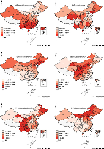
Table 7. Median values and locations of the spatially varying coefficients for each province.

Province	$lnfdev$	Location	$lnloanrate$	Province	$lnfdev$	Location	$lnloanrate$
Anhui	−0.277	A	0.689	Jiangxi	−0.123	B	0.516
Beijing	−0.535	A	0.854	Jilin	−0.486	A	0.867
Chongqing	−0.125	B	0.408	Liaoning	−0.531	A	0.890
Fujian	−0.134	B	0.570	Ningxia	−0.347	A	0.705
Gansu	−0.308	B	0.757	Qinghai	−0.267	B	0.769
Guangdong	−0.058	B	0.386	Shaanxi	−0.314	B	0.635
Guangxi	−0.039	B	0.299	Shandong	−0.457	A	0.826
Guizhou	−0.060	B	0.317	Shanghai	−0.298	B	0.776
Hebei	−0.524	A	0.844	Shanxi	−0.440	A	0.756
Heilongjiang	−0.425	A	0.823	Sichuan	−0.157	B	0.488
Henan	−0.321	A	0.661	Tianjin	−0.527	A	0.857
Hubei	−0.185	B	0.512	Xinjiang	−0.288	B	0.820
Hunan	−0.076	B	0.384	Yunnan	−0.119	B	0.412
Inner Mongolia	−0.506	A	0.829	Zhejiang	−0.226	A	0.700
Jiangsu	−0.342	A	0.777	Hainan	−0.096	B	0.389

A and B denote the location of a province/city is above and below the geographically dividing line, respectively.

4.4. Results of the geographically dividing line

A closer inspection of Figure 2 reflects a clear “northeast‒southwest” spatial pattern with respect to the impact of financial development on carbon emission reduction. That is, the role of financial development in reducing carbon emissions is stronger in the northeastern region due to its negative and larger absolute median values of the estimated spatially varying coefficients, but a weaker impact of financial development is observed in the southwestern region. Interestingly, the above spatial pattern can be approximated by drawing a geographically dividing line connecting the easternmost tip of Xinjiang and the easternmost tip of Fujian, as depicted in Figure 3. Then, all provinces/cities are classified into northeastern provinces/cities above the dividing line with larger impacts of financial development on carbon emission reduction and southwestern provinces/cities below the line where financial development demonstrates smaller impacts on carbon emission reduction. Furthermore, the results of the one-way ANOVA in Table 8 provide statistical evidence (p-value is 0.000) supporting the existence of the geographically dividing line.

Figure 3. Results of the geographically dividing line.

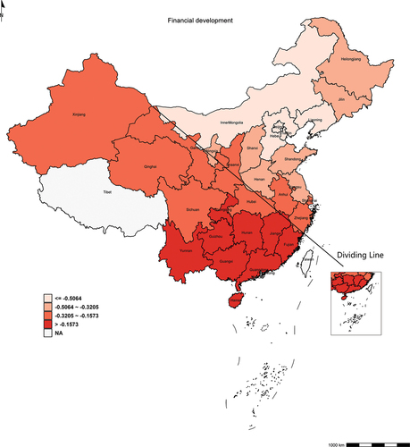
Table 8. One-way analysis of variance (ANOVA).

Source	Sum of squares	Degree of freedom	Mean square	F-statistic	p-value	F-critical value
Between	0.5009	1	0.5009	49.4099	.0000	4.1960
Within	0.2839	28	0.0101
Total	0.7848	29

5. Discussions and implications

The empirical findings of this paper provide policy-makers with profound methodological and managerial implications when developing financial policies for mitigating CO₂ emissions. From the methodological point of view, the superiority of the RE-ESF and RE-ESF-SNVC models has been confirmed by achieving better goodness-of-fit performance than the pooled regression model. That is, the observed spatial effect can be extracted by the Moran eigenvectors and can better characterize the global and local relationships between financial development and CO₂ emissions. This finding suggests the potential application of the RE-ESF and RE-ESF-SNVC models for addressing spatial effects to other air pollutants such as nitrogen oxides (NO_x), sulfur oxides (SO_x), and particulate matter (PM) emissions.

From the managerial point of view, the spatial dependence and heterogeneity of CO₂ emissions driven by financial development encourages policy-makers to develop province-specific and cross-provincial financial policies for mitigating CO₂ emissions. First, at the global level, it is found that financial development can significantly mitigate CO₂ emissions, suggesting the implementation of proactive fiscal and monetary policies to promote financial development. For example, the reserve requirement ratio can be lowered appropriately to increase the total amount of loanable funds. Meanwhile, higher deposit rates and lower tax rates can attract more bank deposits.

Second, at the local level, the contribution of financial development to CO₂ emission mitigation demonstrates clear regional disparities, suggesting province-specific financial policies. That is, more financial resources and policy support can be offered to promote financial development in provinces with greater contributions to CO₂ emission mitigation. However, such contributions are limited by financial constraints due to their positive and spatially heterogeneous impacts on CO₂ emissions. More specifically, more bank loans can influence CO₂ emissions in two different ways. One way is to reduce emissions through a higher level of financial development, and the other way is to increase emissions through a higher level of financial constraints, resulting in inconclusive impacts on CO₂ emissions. Therefore, it is suggested that a balance between financial development and financial constraints should be achieved due to their contrary impacts on CO₂ emissions by closely monitoring the ratio of bank loans to bank deposits.

Third, the impact of financial development on carbon emissions exhibits a clear “northeast‒southwest” spatial pattern that can be approximated by a geographically dividing line connecting the easternmost tip of Xinjiang and the easternmost tip of Fujian. This finding suggests that instead of a one-size-fits-all approach, policy-makers should consider provincial disparities in financial development in reducing carbon emissions and formulate differentiated policies across provinces. More specifically, given the limited financial resources, the credit constraints can be relaxed for the northeastern provinces/cities above the dividing line (e.g., Beijing, Liaoning, Tianjin, Hebei, Inner Mongolia, Jilin) to promote local financial development. At present, the People’s Bank of China’s monetary policy, such as the adjustment of the reserve requirement ratio differentiates among different legal entities (e.g., larger industrial and commercial banks and small village banks) without consideration of regional disparities. Thus, it is concluded that regional monetary policies can be implemented, and national industrial and commercial banks can make reasonable inter-provincial allocations of credit resources in accordance with regional development.

6. Conclusions

To formulate appropriate financial policies for CO₂ emission mitigation, it is essential to better understand the underlying relationships as well as the influential mechanism between financial development and CO₂ emissions. For this purpose, we apply the RE-ESF and RE-ESF-SNVC models to capture their global and local relationships, providing policy-makers with profound implications from a spatial dependence and heterogeneity perspective. Using a provincial panel dataset over the period 1997 − 2017, the main findings are as follows.

First, significant spatial effects of CO₂ emissions are detected by Moran’s I and LM tests, and this should be considered when quantifying the impact of financial development on CO₂ emissions. Second, using Moran eigenvectors to extract spatial effects, the RE-ESF and RE-ESF-SNVC models demonstrate a better fit to the dataset than the pooled panel regression model by achieving higher adjusted R², and lower AIC and BIC. Third, financial development, the factor of interest in this paper, can consistently contribute to CO₂ emission mitigation at both the global and local levels. Moreover, its contributions display clear regional disparities, suggesting the inclusion of spatial heterogeneity when developing financial policies. However, the role of financial development in mitigating CO₂ emissions is limited by financial constraints, exhibiting positive and spatially heterogeneous impacts on CO₂ emissions, suggesting a balance between financial development and financial constraints when expanding bank loans. Finally, a clear “northeast‒southwest” spatial pattern with respect to the impact of financial development on carbon emissions is observed, and this can be approximated by a geographically dividing line connecting the easternmost tip of Xinjiang and the easternmost tip of Fujian.

As noted earlier, profound methodological and managerial implications can be provided to develop province-specific and cross-provincial financial policies for CO₂ emission mitigation. Despite these implications, this paper can still be extended in different ways. First, financial development is represented by the ratio of the sum of bank deposits and bank loans to GDP in the current paper, only considering a country’s bank system and can be extended by including a country’s stock market, bond market and other forms of capital markets. The second way of extending the current work is to explore the spatial linkage between financial development and CO₂ emissions at the city and county levels when more recent and detailed data are available in the future. In addition, the current research can be extended by considering the seasonal characteristics of carbon emissions and discovering the underlying reasons for the geographically dividing line.

Disclosure statement

No potential conflict of interest was reported by the author(s).

Correction Statement

This article has been corrected with minor changes. These changes do not impact the academic content of the article.

Notes

¹ https://www.bp.com/en/global/corporate/energy-economics/statistical-review-of-world-energy.html

² Due to data availability, Tibet, Hong Kong, Macao, and Taiwan are not included. The maps of China’s provincial administrative divisions used in this study are from the 2015 data on China’s provincial administrative boundaries released by the Institute of Geographic Sciences and Natural Resources of the Chinese Academy of Sciences and the Resource and Environmental Science Data Center of the Chinese Academy of Sciences. For the final maps, please refer to the officially released maps.

References

- Abbasi, F., and K. Riaz. 2016. CO2 emissions and financial development in an emerging economy: An augmented VAR approach. Energy Policy 90:102–20. doi:10.1016/j.enpol.2015.12.017.
- Acs, Z. J., L. Anselin, and A. Varga. 2002. Patents and innovation counts as measures of regional production of new knowledge. Research Policy 31 (7):1069–85. doi:10.1016/S0048-7333(01)00184-6.
- Ahmad, M., Z. Khan, Z. U. Rahman, and S. Khan. 2018. Does financial development asymmetrically affect CO2 emissions in China? An application of the nonlinear autoregressive distributed lag (NARDL) model. Carbon Management 9 (6):631–44. doi:10.1080/17583004.2018.1529998.
- Ahmed, F., S. Kousar, A. Pervaiz, and J. P. Ramos-Requena. 2020. Financial development, institutional quality, and environmental degradation nexus: New evidence from asymmetric ARDL co-integration approach. Sustainability 12 (18):7812. doi:10.3390/su12187812.
- Ali, H. S., S. H. Law, W. L. Lin, Z. Yusop, L. Chin, and U. A. A. Bare. 2019. Financial development and carbon dioxide emissions in Nigeria: Evidence from the ARDL bounds approach. GeoJournal 84 (3):641–55. doi:10.1007/s10708-018-9880-5.
- Anselin, L., A. K. Bera, R. Florax, and M. J. Yoon. 1996. Simple diagnostic tests for spatial dependence. Regional Science and Urban Economics 26 (1):77–104. doi:10.1016/0166-0462(95)02111-6.
- Apergis, N., and I. Ozturk. 2015. Testing environmental kuznets curve hypothesis in Asian countries. Ecological Indicators 52:16–22. doi:10.1016/j.ecolind.2014.11.026.
- Bai, J., Q. Jian, Q. Wei, and J. Zeng. 2016. Current situation and trend analysis of carbon dioxide emission from urban and rural residential building at embodies stage in China. Environmental Engineering 34 (10):161–65.
- Bayar, Y., L. D. Maxim, and A. Maxim. 2020. Financial development and CO2 emissions in post-transition European Union countries. Sustainability 12 (7):2640. doi:10.3390/su12072640.
- Chen, P., Y. Lu, Y. Wan, and A. Zhang. 2021. Assessing carbon dioxide emissions of high-speed rail: The case of Beijing-Shanghai corridor. Transportation Research, Part D: Transport & Environment 97:102949. doi:10.1016/j.trd.2021.102949.
- De Hoyos, R. E., and V. Sarafidis. 2006. Testing for cross-sectional dependence in panel-data models. The Stata Journal 6 (4):482–96. doi:10.1177/1536867X0600600403.
- Dietz, T., and E. A. Rosa. 1997. Effects of population and affluence on CO2 emissions. Proceedings of the National Academy of Sciences of the United States of America 94 (1):175–79. doi:10.1073/pnas.94.1.175.
- Dogan, E., and F. Seker. 2016. The influence of real output, renewable and non-renewable energy, trade and financial development on carbon emissions in the top renewable energy countries. Renewable and Sustainable Energy Reviews 60:1074–85. doi:10.1016/j.rser.2016.02.006.
- Farhani, S., and I. Ozturk. 2015. Causal relationship between CO2 emissions, real GDP, energy consumption, financial development, trade openness, and urbanization in Tunisia. Environmental Science and Pollution Research 22 (20):15663–76. doi:10.1007/s11356-015-4767-1.
- Fotheringham, A. S., R. Crespo, and J. Yao. 2015. Geographical and temporal weighted regression (GTWR). Geographical Analysis 47 (4):431–52. doi:10.1111/gean.12071.
- Fotheringham, A. S., W. Yang, and W. Kang. 2017. Multiscale geographically weighted regression (MGWR). Annals of the American Association of Geographers 107 (6):1247–65. doi:10.1080/24694452.2017.1352480.
- Griffith, D. A. 2003. Spatial autocorrelation and spatial filtering: Gaining understanding through theory and scientific visualization. Springer Science & Business Media. doi:10.1007/978-3-540-24806-4_4.
- Griffith, D. A. 2009. Modeling spatial autocorrelation in spatial interaction data: Empirical evidence from 2002 Germany journey-to-work flows. Journal of Geographical Systems 11 (2):117–40. doi:10.1007/s10109-009-0082-z.
- Guo, M., and Y. Hu. 2020. The impact of financial development on carbon emission: Evidence from China. Sustainability 12 (17):6959. doi:10.3390/su12176959.
- Haseeb, A., E. Xia, Danish, M. A. Baloch, and K. Abbas. 2018. Financial development, globalization, and CO2 emission in the presence of EKC: Evidence from BRICS countries. Environmental Science and Pollution Research 25 (31):31283–96. doi:10.1007/s11356-018-3034-7.
- Huang, B., B. Wu, and M. Barry. 2010. Geographically and temporally weighted regression for modeling spatio-temporal variation in house prices. International Journal of Geographical Information Science 24 (3):383–401. doi:10.1080/13658810802672469.
- Jalil, A., and M. Feridun. 2011. The impact of growth, energy and financial development on the environment in China: A cointegration analysis. Energy Economics 33 (2):284–91. doi:10.1016/j.eneco.2010.10.003.
- Javid, M., and F. Sharif. 2016. Environmental kuznets curve and financial development in Pakistan. Renewable and Sustainable Energy Reviews 54:406–14. doi:10.1016/j.rser.2015.10.019.
- Ji, Z. 2013. Research on regional differences in loan-to-deposit ratio based on commercial bank branch data. Financial Research 9:12–31.
- Kao, C. 1999. Spurious regression and residual-based tests for cointegration in panel data. Journal of Econometrics 90 (1):1–44. doi:10.1016/S0304-4076(98)00023-2.
- Kim, D. H., Y. C. Wu, and S. C. Lin. 2020. Carbon dioxide emissions and the finance curse. Energy Economics 88:104788. doi:10.1016/j.eneco.2020.104788.
- Lahiani, A. 2020. Is financial development good for the environment? An asymmetric analysis with CO2 emissions in China. Environmental Science and Pollution Research 27 (8):7901–09. doi:10.1007/s11356-019-07467-y.
- Lantz, V., and Q. Feng. 2006. Assessing income, population, and technology impacts on CO2 emissions in Canada: Where’s the EKC? Ecological Economics 57 (2):229–38. doi:10.1016/j.ecolecon.2005.04.006.
- LeSage, J., and R. K. Pace. 2009. Introduction to spatial econometrics. New York: Chapman and Hall/CRC.
- Li, Y., Y. Cui, B. Cai, J. Guo, T. Cheng, and F. Zheng. 2020. Spatial characteristics of CO2 emissions and PM2.5 concentrations in China based on gridded data. Applied Energy 266:114852. doi:10.1016/j.apenergy.2020.114852.
- Liu, H., and G. Gong. 2022. Heterogeneous impacts of financial development on carbon emissions: Evidence from China’s provincial data. Environmental Science and Pollution Research 29 (25):37565–81. doi:10.1007/s11356-021-18209-4.
- Lv, Z., and S. Li. 2021. How financial development affects CO2 emissions: A spatial econometric analysis. Journal of Environmental Management 277:111397. doi:10.1016/j.jenvman.2020.111397.
- Moghadam, H. E., and V. Dehbashi. 2018. The impact of financial development and trade on environmental quality in Iran. Empirical Economics 54 (4):1777–99. doi:10.1007/s00181-017-1266-x.
- Moran, P. A. P. 1948. The interpretation of statistical maps. Journal of the Royal Statistical Society, Series B (Methodological) 10 (2):243–51. doi:10.1111/j.2517-6161.1948.tb00012.x.
- Murakami, D., and D. A. Griffith. 2015. Random effects specifications in eigenvector spatial filtering: A simulation study. Journal of Geographical Systems 17 (4):311–31. doi:10.1007/s10109-015-0213-7.
- Murakami, D., and D. A. Griffith. 2019. Spatially varying coefficient modeling for large datasets: Eliminating N from spatial regressions. Spatial Statistics 30:39–64. doi:10.1016/j.spasta.2019.02.003.
- Murakami, D., and D. A. Griffith (2020). Balancing spatial and non-spatial variation in varying coefficient modeling: A remedy for spurious correlation. arXiv preprint arXiv:2005.09981.
- Murakami, D., T. Yoshida, H. Seya, D. A. Griffith, and Y. Yamagata. 2017. A Moran coefficient-based mixed effects approach to investigate spatially varying relationships. Spatial Statistics 19:68–89. doi:10.1016/j.spasta.2016.12.001.
- Nasir, M. A., T. L. D. Huynh, and H. T. X. Tram. 2019. Role of financial development, economic growth & foreign direct investment in driving climate change: A case of emerging ASEAN. Journal of Environmental Management 242:131–41. doi:10.1016/j.jenvman.2019.03.112.
- Nasreen, S., and S. Anwar. 2015. The impact of economic and financial development on environmental degradation: An empirical assessment of EKC hypothesis. Studies in Economics and Finance 32 (4):485–502. doi:10.1108/SEF-07-2013-0105.
- Neog, Y., and A. K. Yadava. 2020. Nexus among CO2 emissions, remittances, and financial development: A NARDL approach for India. Environmental Science and Pollution Research 27 (35):44470–81. doi:10.1007/s11356-020-10198-0.
- Omri, A., S. Daly, C. Rault, and A. Chaibi. 2015. Financial development, environmental quality, trade and economic growth: What causes what in MENA countries. Energy Economics 48:242–52. doi:10.1016/j.eneco.2015.01.008.
- Oshan, T. M., and A. S. Fotheringham. 2018. A comparison of spatially varying regression coefficient estimates using geographically weighted and spatial-filter-based techniques. Geographical Analysis 50 (1):53–75. doi:10.1111/gean.12133.
- Oshan, T., L. J. Wolf, A. S. Fotheringham, W. Kang, Z. Li, and H. Yu. 2019. A commenton geographically weighted regression with parameter-specific distance metrics. International Journal of Geographical Information Science 33 (7):1289–99. doi:10.1080/13658816.2019.1572895.
- Ozturk, I., and A. Acaravci. 2013. The long-run and causal analysis of energy, growth, openness and financial development on carbon emissions in Turkey. Energy Economics 36:262–67. doi:10.1016/j.eneco.2012.08.025.
- Pata, U. K. 2018. Renewable energy consumption, urbanization, financial development, income and CO2 emissions in Turkey: Testing EKC hypothesis with structural breaks. Journal of Cleaner Production 187:770–79. doi:10.1016/j.jclepro.2018.03.236.
- Rojas-Suarez, L., and S. Weisbrod. 1996. Banking crises in Latin America: Experiences and issues. Banking Crises in Latin America 3–21. doi:10.2139/ssrn.1815951.
- Saidi, K., and M. B. Mbarek. 2017. The impact of income, trade, urbanization, and financial development on CO2 emissions in 19 emerging economies. Environmental Science and Pollution Research 24 (14):12748–57. doi:10.1007/s11356-016-6303-3.
- Salahuddin, M., K. Alam, I. Ozturk, and K. Sohag. 2018. The effects of electricity consumption, economic growth, financial development and foreign direct investment on CO2 emissions in Kuwait. Renewable and Sustainable Energy Reviews 81:2002–10. doi:10.1016/j.rser.2017.06.009.
- Salahuddin, M., J. Gow, and I. Ozturk. 2015. Is the long-run relationship between economic growth, electricity consumption, carbon dioxide emissions and financial development in gulf cooperation council countries robust? Renewable and Sustainable Energy Reviews 51:317–26. doi:10.1016/j.rser.2015.06.005.
- Shahbaz, M., Q. M. A. Hye, A. K. Tiwari, and N. C. Leitão. 2013. Economic growth, energy consumption, financial development, international trade and CO2 emissions in Indonesia. Renewable and Sustainable Energy Reviews 25:109–21. doi:10.1016/j.rser.2013.04.009.
- Shahbaz, M., S. A. Solarin, H. Mahmood, and M. Arouri. 2013. Does financial development reduce CO2 emissions in Malaysian economy? A time series analysis. Economic Modelling 35:145–52. doi:10.1016/j.econmod.2013.06.037.
- Shahbaz, M., A. K. Tiwari, and M. Nasir. 2013. The effects of financial development, economic growth, coal consumption and trade openness on CO2 emissions in South Africa. Energy Policy 61:1452–59. doi:10.1016/j.enpol.2013.07.006.
- Shan, Y., Q. Huang, D. Guan, and K. Hubacek. 2020. China CO2 emission accounts 2016–2017. Scientific Data 7 (1):1–9. doi:10.1038/s41597-020-0393-y.
- Tamazian, A., J. P. Chousa, and K. C. Vadlamannati. 2009. Does higher economic and financial development lead to environmental degradation: Evidence from BRIC countries. Energy Policy 37 (1):246–53. doi:10.1016/j.enpol.2008.08.025.
- Tang, Z., Z. Mei, and J. Zou. 2021. Does the opening of high-speed railway lines reduce the carbon intensity of China’s resource-based cities? Energies 14 (15):4648. doi:10.3390/en14154648.
- Xiong, F., L. Zang, D. Feng, and J. Chen. 2023. The influencing mechanism of financial development on CO2 emissions in China: Double moderating effect of technological innovation and fossil energy dependence. Environment, Development and Sustainability 25 (6):4911–33. doi:10.1007/s10668-022-02250-5.
- Xu, H., J. Cao, J. C. Chow, R. J. Huang, Z. Shen, L. W. A. Chen, K. F. Ho, and J. H. Watson. 2016. Inter-annual variability of wintertime PM2.5 chemical composition in Xi’an, China: Evidences of changing source emissions. Science of the Total Environment 545-546:546–55. doi:10.1016/j.scitotenv.2015.12.070.
- Yang, F., K. Li, M. Jin, and W. Shi. 2021. Does financial deepening drive spatial heterogeneity of PM2.5 concentrations in China? New evidence from an eigenvector spatial filtering approach. Journal of Cleaner Production 291 (April):125945. doi: 10.1016/j.jclepro.2021.125945.
- Yan, W., and D. Sheng. 2014. Trade openness, technological progress and my country’s human capital investment. International Trade Issues 6:10.
- Yazdi, S. K., and E. G. Beygi. 2018. The dynamic impact of renewable energy consumption and financial development on CO2 emissions: For selected African countries. Energy Sources, Part B: Economics, Planning, & Policy 13 (1):13–20. doi:10.1080/15567249.2017.1377319.
- You, W., and Z. Lv. 2018. Spillover effects of economic globalization on CO2 emissions: A spatial panel approach. Energy Economics 73:248–57. doi:10.1016/j.eneco.2018.05.016.
- Yuan, M., Y. Huang, H. Shen, and T. Li. 2018. Effects of urban form on haze pollution in China: Spatial regression analysis based on PM2.5 remote sensing data. Applied Geography 98:215–23. doi:10.1016/j.apgeog.2018.07.018.
- Yuan, H., T. Zhang, Y. Feng, Y. Liu, and X. Ye. 2019. Does financial agglomeration promote the green development in China? A spatial spillover perspective. Journal of Cleaner Production 237:117808. doi:10.1016/j.jclepro.2019.117808.
- Yu, D., D. Murakami, Y. Zhang, X. Wu, D. Li, X. Wang, and G. Li. 2020. Investigating high-speed rail construction’s support to county level regional development in China: An eigenvector based spatial filtering panel data analysis. Transportation Research Part B: Methodological 133:21–37. doi:10.1016/j.trb.2019.12.006.
- Zaidi, S. A. H., M. W. Zafar, M. Shahbaz, and F. Hou. 2019. Dynamic linkages between globalization, financial development and carbon emissions: Evidence from Asia Pacific economic cooperation countries. Journal of Cleaner Production 228:533–43. doi:10.1016/j.jclepro.2019.04.210.
- Zhang, Y. J. 2011. The impact of financial development on carbon emissions: An empirical analysis in China. Energy Policy 39 (4):2197–203. doi:10.1016/j.enpol.2011.02.026.
- Zhang, W., M. Hong, J. Li, and F. Li. 2021. An examination of green credit promoting carbon dioxide emissions reduction: A provincial panel analysis of China. Sustainability 13 (13):7148. doi:10.3390/su13137148.
- Zhao, B., and W. Yang. 2020. Does financial development influence CO2 emissions? A Chinese province-level study. Energy 200:117523. doi:10.1016/j.energy.2020.117523.
- Zhou, H., S. Qu, Q. Yuan, and S. Wang. 2020. Spatial effects and nonlinear analysis of energy consumption, financial development, and economic growth in China. Energies 13 (18):4982. doi:10.3390/en13184982.
- Zhou, Y., Y. Xu, C. Liu, Z. Fang, and J. Guo. 2019. Spatial effects of technological progress and financial support on China’s provincial carbon emissions. International Journal of Environmental Research and Public Health 16 (10):1743. doi:10.3390/ijerph16101743.
- Zhou, X., and H. Zhang. 2023. Does financial development benefit carbon neutrality in China? Pathway analysis and empirical study. Applied Economics 1–22. doi:10.1080/00036846.2023.2168610.