Plug-in hybrid electric vehicle observed utility factor: Why the observed electrification performance differ from expectations

Abstract

Plug-in hybrid electric vehicles (PHEVs) are an effective vehicle technology to reduce light duty vehicle greenhouse gas emissions and gasoline consumption. They combine all-electric driving capabilities of a battery electric vehicle with the engine downsizing and fuel economy improvements of a hybrid electric vehicle. Their environmental performance is predicated upon the metric utility factor (UF). It is formally defined in the Society of Automotive Engineers J2841 standard and denotes the fraction of vehicle miles traveled (VMT) on electricity (eVMT). Using year-long driving and charging data collected from 153 PHEVs in California with 11–53 miles range, this article systematically evaluates what aspects of driving and charging behavior causes observed UF to deviate from J2841 expectations. Our analyses indicated that charging behavior, distribution of daily VMT, efficiency of electrical energy consumption in the charge depleting (CD) mode, and annual VMT were the major factors contributing to the disparities between observed and expected UF. The direction and magnitude of their individual effect varied with the vehicle type and range. Approximately ±45% of deviations from J2841 UF is attributable to the observed charging behavior. Differences in daily VMT distribution were responsible for −20% to +3% of deviation. Annual VMT and effective CD range achieved on-road influenced the UF deviation by ±25% and −20% to −4%, respectively.

Keywords:

• Electrification potential
• longitudinal data
• plug-in hybrid electric vehicle
• utility factor

1. Introduction

The transportation sector is responsible for 30% of the U.S. total greenhouse gas (GHG) emissions and light duty vehicles (LDVs) account for close to 60% of the transport sector GHG emissions (U.S. Environmental Protection Agency [EPA], 2019a). Light duty vehicle (LDV) electrification is a promising solution to mitigate the adverse impacts of GHG emissions on the environment and public health. Plug-in hybrid electric vehicles (PHEVs) are often considered a viable option to catalyze the transition toward LDV electrification (Cordera et al., 2019; Poullikkas, 2015). PHEVs are equipped with a larger battery pack compared to conventional hybrid vehicles (HEVs) that can be charged using grid electricity and have an internal combustion engine (ICE). PHEVs are not limited by the range of the battery and combine the advantages all-electric capabilities of a battery electric vehicle (BEV) with the engine downsizing, minimal energy losses due to no engine idling, and regenerative braking capabilities of a HEV. PHEVs are operated in two distinct modes: charge depleting (CD), when electrical energy stored in the battery after charging is used to propel the vehicle and charge sustaining (CS) mode in which the PHEV is driven on gasoline.

CD mode can be categorized into CD-EV and CD-blended (CDB) modes. In the CD-EV mode of operation, the entire traction energy is met by discharging the energy stored in the battery. The vehicle is driven in all-electric mode by the motor and the engine is never turned on. This type of operation is called EV-mode, all-electric mode, or zero emission (ZE) mode because only electricity is consumed and there are no tail-pipe emissions. Depending on the powertrain configuration, road network topology, speed and acceleration characteristics, in the CD mode, engine may turn on to partially assist the motor in meeting the total energy demand at the wheels. This is called CDB mode of operation because both electricity and gasoline are consumed. The CD mode of operation continues until the battery is fully discharged, after which the PHEV is operated in the CS mode as a regular HEV with the ICE providing the propulsion energy and only gasoline is consumed. Operational and fuel use flexibility enables PHEVs to substitute gasoline partially or completely with electricity. It is this same attractive design feature that makes the exercise of characterizing PHEV emissions and energy consumption quite challenging. The test procedures for estimating their environmental performance need to combine both modes of operation.

The distance driven in either CD or CS modes depends on battery capacity, electrical energy consumed in the CD mode, distribution of trip lengths and frequencies, and the recharging frequency. A key performance metric of PHEVs from the perspective of gasoline displacement, GHG emissions, and local criteria pollutants is the fraction VMT electrified, also known as utility factor (UF). At a conceptual level as the name implies, it denotes the limited utility of the CD mode of operation until the battery is fully depleted, hence called UF. Society of Automotive Engineers (SAE) J2841 (J2841, 2010) formally defines the UF and outlines recommended procedures to calculate the UF. UF essentially weighs the share of distance driven in CD and CS mode of operation relative to the total distance traveled and is expressed as a ratio between 0 and 1. These weights are incorporated into the test procedures for estimating combined fuel economy, and mode specific emissions and energy consumption according to the SAE J1711 (J1711, 2010) standard.

PHEVs are typically denoted as PHEVX, where “X” is the charge depleting range (R_CD) or simply range in miles, where R_CD is the distance traveled by a fully charged PHEV in the CD mode before the battery is completely depleted. The vehicle miles traveled (VMT) in the CD mode could be comprised of VMT on electricity (eVMT) only or electricity and gasoline (gVMT), whereas CS mode involves only gVMT. There are four different definitions of range in the SAE J1711–All Electric Range (AER), CD Cycle Range, CD Actual Range, and Equivalent All Electric Range. The AER of a PHEV is the total distance traveled from the beginning of a full charge test (FCT) to the point when the first engine turn-on event occurs. The CD cycle range (R_CDC) is the distance traveled either completely (no engine turn-on) in the CD-EV mode or partially in the CDB mode under a test-cycle until the battery is completely depleted. The CD cycle range is the sum of the distances traveled from the beginning of an FCT up until the end of the last test-cycle(s) prior to the cycle meeting the End-of Test (EOT) criterion including the transition range where the engine might momentarily turn on although the battery is not fully depleted. The EPA label lists the AER and R_CDC for applicable PHEV models. Full charge test as the name implies requires that the test begin with the battery state of charge (SOC) of 100% and transition range is the distance traveled between the CD and CS modes. Since the exact determination of the point at which the transition between CD and CS modes occur, the SAE J1711 employs analytical method to determine the CD actual range (R_CDA) which is always less than or equal to the R_CDC. The Equivalent All Electric Range (EAER) is the fraction of CD cycle range attributable to grid electricity and is equal to greater than the AER.

The J2841 UF definitions for PHEVs explicitly assume that:

1. travel day starts with a fully charged battery.

2. PHEV is charged once per day on days driven after the end of last trip.

3. impact of additional intra-day charging, and vehicle not being charged at the end of travel day offset each other equally, and

4. travel patterns of PHEVs are identical to the single-day trip diary information of ICEs in the 2001 National Household Travel Survey (NHTS).

These assumptions have widespread ramifications on energy and emissions estimates of PHEVs embodied in existing policies, charging infrastructure planning, and electricity grid impact studies (Davies & Kurani, 2013; Tal et al., 2014; Wang et al., 2011; Wood et al., 2018; Zhou et al., 2016). In the policy domain, the significance of the UF cannot be understated since it is the critical metric assessed for many policies in the United States including the Environmental Protection Agency (EPA) fuel economy labeling or window sticker (Duoba & Bocci, 2009; Gonder & Simpson, 2007), credit allocations under California’s Zero Emission Vehicle (ZEV) mandate and Low Carbon Fuel Standard (California Air Resources Board [CARB], 2017b), and compliance with fuel economy and emission standards (Aviquzzaman, 2014; Bradley & Davis, 2011; Bradley & Quinn, 2010). Although the SAE J2841 was developed from a U.S. centric perspective, at a methodological level, the concept of UF, core assumptions on charging behavior, relying on national driving statistics to represent PHEV driving patterns, and a standardized procedure to calculate the UF has been adopted by regions outside the United States as well, albeit with few region specific modifications to the test cycles and driving database. China’s LDV fuel economy standards and energy consumption and emission estimates for type approval in European Union (European Commission, 2018; Hao et al., 2020), to name a few.

The assumptions outlined in the J2841, although plausible, may not reflect how actual PHEV owners drive and charge their vehicles. Prior work in this area focused on alternative UF calculated using different cross-sectional or longitudinal travel survey datasets, incorporating additional charging scenarios, and performing sensitivity analysis of UF to various vehicle and sociodemographic attributes (Aviquzzaman, 2014; Bradley & Davis, 2011; Bradley & Quinn, 2010; Gonder et al., 2007; Grahn et al., 2014; Neubauer & Wood, 2014). More recently, with the availability of observed driving and charging data through on-board telematics and data-loggers (Björnsson & Karlsson, 2017; Bradley & Frank, 2009; Crain et al., 2016; Davies & Kurani, 2010; Smart et al., 2010, 2013, 2014), estimating on-road emission mitigation potential and characterizing driving and charging patterns (Duhon et al., 2015; Figenbaum & Weber, 2018; Lee et al., 2011; Plötz et al., 2015, 2017) are other areas where analysis of UF is pertinent. UF has also been widely used in evaluating the life-cycle costs, emissions and value proposition of PHEVs (Karabasoglu & Michalek, 2013; Neubauer et al., 2013), and optimal battery size design and its impact on market acceptance (Björnsson et al., 2018; Tamor et al., 2013).

In summary, many studies have been carried out to assess validity of J2841 UF assumptions on charging and driving by simulating different scenarios and comparing simulated UF to their theoretical J2841 UF equivalent. However, a straightforward approach that uses observed driving and charging behavior to reconcile their deviations from J2841 UF expectations is found lacking. To the best of our knowledge, no study attempted to delve deep into how key driving and charging traits such as annual VMT; daily VMT (DVMT) distribution and range utilization; charging behavior; and effective range achieved on-road, affect the disparities between observed UF and J2841 UF. Data availability of actual PHEVs is still scarce compared to the publicly available travel survey data of conventional ICEs. Though observed data is valuable and desirable since they represent PHEV usage better compared to surveys, policy recommendations cannot be tailored and altered depending on the availability and quality of actual PHEV usage data. Therefore, it is necessary to interpret the UF observed in terms of the standardized UF. This article addresses these two areas of need in the context of UF of PHEVs using year-long GPS enabled driving and charging data of 153 PHEVs (11–53 miles range) in California.

The objectives of this article are:

1. quantitatively and qualitatively understand the deviations in observed UF from J2841 UF.

2. identify vital aspects of driving and charging that cause these deviations and;

3. systematically estimate the direction and magnitude of impact individually attributable to these aspects.

The outcomes of this work will augment policy insights gathered from contemporary efforts and elucidate how observations about PHEV usage today can better inform future vehicle design and policy needs. This study contributes to the evolving field of improving the accuracy of UF estimates to enhance PHEV emissions reduction benefits and market penetration. Furthermore, the methodology outlined in this article is intended to serve as a template for similar comparisons of PHEVs performance in different locations and settings using different standards. Rest of the article is organized as follows. In Section 2, we briefly review the background of the standardized J2841 UF and the alternative definitions considered in literature. A concise overview of its developments in the European Union (EU), South Korea, Japan, and China is also presented in Section 2. Section 3 provides an overview of the data and analytical methods employed in this article to quantify deviations between observed and J2841 UF. Results are elaborated in Section 4. We discuss our findings and its consequences in Section 5.

2. J2841 UF in practice and its variants

In this section, we describe the foundational and procedural aspects of the SAE J2841 UF within the U.S. context. We then broaden the scope and provide an overview of its how it’s estimated outside the United States, specifically in EU, South Korea, Japan and China and summarize contemporary literature on UF and its variants.

2.1. Conventional J2841 UF definitions

The J2841 UF is calculated based on the trip and daily VMT distribution of mainstream ICE users in the United States represented in the 2001 NHTS (Hu & Reuscher, 2004). The NHTS trip diary information captures a one-day snapshot of travel patterns self-reported by survey respondents. The raw trip file has close to 642,000 trips and the following filters are applied to calculate the UF: (i) subject was driver on this trip (DRVR_FLG = 1); (ii) national sample (SMPLSRCE = 1); (iii) non-zero trip miles and duration (TRPMILES and TRVL_MIN > 0); and (iv) only light duty vehicle trips (VEHTYPE is 1–4) are selected. DVMT is obtained by summing the trip distance and time for each unique household and vehicle used and roughly 32,000 vehicles or vehicle-days are in the filtered subset. Let $d\left(k\right)$ denote the distance traveled on travel day k. The VMT weighted daily distance-based UF according to the J2841 methodology is calculated as follows: If $d\left(k\right)>R_{\mathrm{CD}},$ then UF =1 and $R_{\mathrm{CD}}/d\left(k\right)$ otherwise. For a travel dataset with N days, the same logic is extended and the UF for a specific range is calculated according to Equation (1)(1) $$\mathrm{UF}\left(R_{\mathrm{CD}}\right)=\frac{{\sum }_{k-1}^N\min \left(d\left(k\right),R_{\mathrm{CD}}\right)\mathrm{ }}{{\sum }_{k-1}^{N}d\left(k\right)}\mathrm{ }$$(1) . (1) $$\mathrm{UF}\left(R_{\mathrm{CD}}\right)=\frac{{\sum }_{k-1}^N\min \left(d\left(k\right),R_{\mathrm{CD}}\right)\mathrm{ }}{{\sum }_{k-1}^{N}d\left(k\right)}\mathrm{ }$$(1)

The VMT weighted UF described in Equation (1)(1) $$\mathrm{UF}\left(R_{\mathrm{CD}}\right)=\frac{{\sum }_{k-1}^N\min \left(d\left(k\right),R_{\mathrm{CD}}\right)\mathrm{ }}{{\sum }_{k-1}^{N}d\left(k\right)}\mathrm{ }$$(1) is called the fleet utility factor (FUF) since represents the UF of an entire fleet of PHEVs. The numerator and denominator in Equation (1)(1) $$\mathrm{UF}\left(R_{\mathrm{CD}}\right)=\frac{{\sum }_{k-1}^N\min \left(d\left(k\right),R_{\mathrm{CD}}\right)\mathrm{ }}{{\sum }_{k-1}^{N}d\left(k\right)}\mathrm{ }$$(1) are the total eVMT and VMT of the fleet. The FUF represents the fraction of total miles in the NHTS fleet driven in the CD mode. In some instances, it might be desirable to convey information for an average PHEV since the VMT weighted FUF is biased toward long-distance trips. For this purpose, the individual utility factor (IUF) is used which is the vehicle weighted UF. The basic approach to calculate the IUF is same as that of the FUF. Let N_Days and N_Vehicles denote the number of days and vehicles in the dataset and d_(i,j) denote the distance traveled by vehicle i on travel day j. The IUF is calculated according to Equation (2)(2) $$\mathrm{IUF}\left(R_{\mathrm{CD}}\right)=\frac{\sum _{i=1}^{N\mathrm{Vehicles}}\frac{{\sum }_{j=1}^{N\mathrm{Days}}\min \left(d_{i,j},R_{\mathrm{CD}}\right) }{{\sum }_{j=1}^{N\mathrm{Days}}{d}_{i,j}}}{N\mathrm{Vehicles}}$$(2) . The IUF represents the arithmetic mean of the fraction of miles driven in CD mode over N_Vehicles. Depending on the whether the dataset has information about single day (SD) or multiple days (MD) of travel, the IUF calculated is expressed as SDIUF or MDIUF. The Commute Atlanta dataset (Elango et al., 2007) was used as a supplementary dataset to calculate the MDIUF but the FUF and IUF distribution was found to be the same between them. (2) $$\mathrm{IUF}\left(R_{\mathrm{CD}}\right)=\frac{\sum _{i=1}^{N\mathrm{Vehicles}}\frac{{\sum }_{j=1}^{N\mathrm{Days}}\min \left(d_{i,j},R_{\mathrm{CD}}\right) }{{\sum }_{j=1}^{N\mathrm{Days}}{d}_{i,j}}}{N\mathrm{Vehicles}}$$(2)

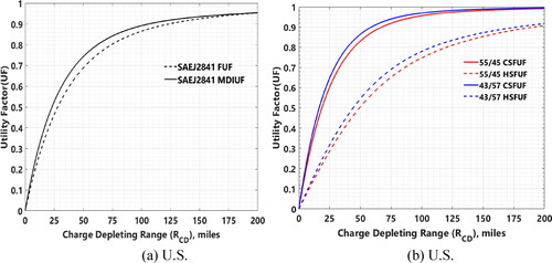
Since energy consumption is a function of driving speed, the J2841 method includes two methods to create FUF that are conditional upon driving style: City Specific (CSFUF) or Highway Specific (HSFUF). In the first method, average trip speed is calculated, and the entire trip is categorized as city or highway driving based on a cutoff speed. The conventional assumption on the split between city and highway driving is 55/45 (U.S. EPA, 2006) and the cutoff speed to obtain this is 42 mph. Trips with average speed greater than 42 mph are designated as highway driving and assigned a highway weight of 1 and city weight of 0 and vice-versa for the remaining trips designated as city driving. The second method selects two cutoff speeds to define city only and highway only. Trips with average speed below 25 mph or above 60 mph are categorized as city only and highway only, respectively. The city/highway weight assignment is like the first method. For trips with average speed between the two cutoffs, the city/highway weight is linearly scaled between 0 and 1, wherein the weight for city driving decreases from 1 with increasing speed beyond 25 mph and vice-versa for the highway driving weights. These trips are considered to have an equal likelihood of being city or highway style driving. At a travel day level, daily weights for city driving and highway driving are calculated based on the method chosen and the share of distance traveled in the respective driving style as a ratio of the total daily distance traveled. The dataset is divided into city and highway driving styles and the UF is estimated according to the basic form shown in Equation (1)(1) $$\mathrm{UF}\left(R_{\mathrm{CD}}\right)=\frac{{\sum }_{k-1}^N\min \left(d\left(k\right),R_{\mathrm{CD}}\right)\mathrm{ }}{{\sum }_{k-1}^{N}d\left(k\right)}\mathrm{ }$$(1) . The J2841 method applies exponential fits to the generate FUF and IUF curves, Equation (3)(3) $$\mathrm{UF}\left(x\right)=1-\exp \left[-\left(\sum _{i=1}^j{C_i\left(\frac{x}{D_n}\right)}^i\right)\right]$$(3) , where x is the R_CD, $C_i$ is the fit coefficient, j is 6 for FUF and 10 for IUF, and D_n is the normalized distance (400 miles in the United States). The J2841 FUF and MDIUF, CSFUF, and HSFUF curves are shown in Figure 1(a,b), respectively. (3) $$\mathrm{UF}\left(x\right)=1-\exp \left[-\left(\sum _{i=1}^j{C_i\left(\frac{x}{D_n}\right)}^i\right)\right]$$(3)

Figure 1. Top left (a) U.S. J2841 FUF and MDIUF curves; top right (b) U.S. J2841 CSFUF and HSFUF curves for 55/45 and 43/57 city/highway driving splits.

2.2. UF developments and applications internationally

The concept of UF, its purpose as a weighing factor and as an indicator of the environmental impact of PHEVs, and the basic procedure to estimate the UF outlined in the SAE J2841 is also used as guideline to calculate energy consumption and emissions of PHEVs outside the United States. To account for the country-specific driving patterns and prevailing regulations, representative national driving statistics, test cycles, and testing procedure used outside the United States typically differ from the conventional SAE J1711 and SAE J2841 approach. Quality, sample size, and resolution of national driving database, pre-conditioning requirements (e.g. soak time and temperature, test site conditions), end-of-test criterion, number of test cycles used for CD range determination, and city/highway driving split are some of the aspects that varies outside the United States in regards to UF determination and regulatory assessment of PHEVs (Riemersma & Mock, 2017). A detailed cross-country comparative assessment of UF estimations is outside the scope of this article, therefore we limit our review of international studies to highlighting only its key features.

In the United States two test cycles are used, the Urban Dynamometer Driving Schedule (UDDS) and Highway Fuel Economy Test (HWFET) cycle. In the EU, only one test cycle, namely the Worldwide Harmonized Light-duty vehicle Test Cycle (WLTC) and its associated Worldwide Harmonized Light-duty vehicle Test Procedure (WLTP) are used (European Commission, 2018, 2016a). Prior to the introduction of WLTP in 2017, New European Drive Cycle (NEDC) was used as the test cycle for type approval (Ligterink et al., 2016) but was phased out in favor of the WLTP to reduce the gap between on-road and type approval energy consumption and emission estimates. Realistic driving behavior, inclusion of diverse driving situations (urban, suburban, main road, and motorway), representing high speed and propulsion power demand, and stringent testing conditions are some of the notable benefits of the WLTP compared to the NEDC (ACEA, 2017). The CD range estimated based on the NEDC is reduced by 25% under the WLTP (European Commission, 2016b). Measurements using the WLTP also considers optional equipment and add-ons for comfort, luxury, and performance that impacts the rolling resistance, vehicle aero-dynamics, and mass (European Commission [EC], 2017).

The WLTP is subdivided into four-phases (low, medium, high, and extra high) with the average speeds increasing with each subsequent phase representative of urban (up to 35 mph), suburban (up to 47 mph), main road(up to 60 mph), and motorway (up to 81 mph) driving, respectively. Energy consumption (fuel and electricity) is calculated in each phase and aggregated based on the phase specific UF also known as fractional UF, to determine the combined energy consumption. Currently two datasets are available in the EU to obtain representative driving patterns – European WLTP database which was used to develop the WLTC and the driving data provided by FIAT (European Commission [EC], 2016a). The single overnight charging at home and travel day starting on a fully charged battery assumption is retained in the WLTP for UF estimation in the EU. The WLTP allows EU member nations to develop their own UF curves.

In Japan, prior to 2020, JC08 was the official test cycle, which is set to be replaced by the WLTP as part of its 2030 fuel economy standards for LDVs (ICCT, 2019). The procedure to estimate the UF of PHEVs in Japan is identical to that of the EU’s approach discussed above. China is currently developing its own LDV test cycle called the China Light-duty vehicle test cycle (CLTC) and it is expected to be the norm from 2023 onwards. Between now and 2023, the WLTP will be used for estimating the UF. South Korea follows the SAE J1711 testing procedure and SAE J2841 for UF estimation (Choi et al., 2020; European Commission [EC], 2014).

Equation (4)(4) $${UF}_j\left(x_p\right)=1-\exp \left[-\left(\sum _{\mathrm{j}=1}^k{C_j\left(\frac{x_p}{D_n}\right)}^i\right)\right]-\sum _{\mathrm{l}=1}^{p-1}{UF}_l$$(4) shows the WLTP-based approach for UF estimation in the EU where – ${UF}_j\left(x_p\right)$ is the fractional UF for phase p, $x_p$ is the distance driven in km from the beginning of the full charge test to the end of phase p, $C_j$ 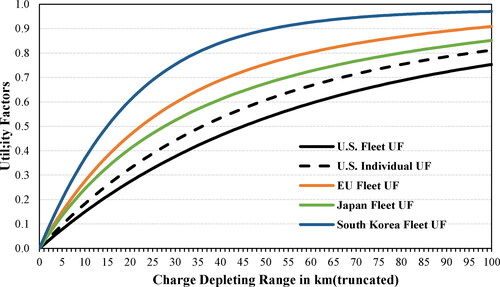is the jth coefficient, k is the order of the exponential fit (10 in EU, 5 in South Korea and 6 in Japan), D_n is the normalized distance, set at 800 km, 600 km, 400 km in the EU, South Korea, and Japan, respectively, and ${\sum }_{\mathrm{l}=1}^{p-1}{UF}_l$ is the sum of calculated UF to phase p – 1. (4) $${UF}_j\left(x_p\right)=1-\exp \left[-\left(\sum _{\mathrm{j}=1}^k{C_j\left(\frac{x_p}{D_n}\right)}^i\right)\right]-\sum _{\mathrm{l}=1}^{p-1}{UF}_l$$(4)

Figure 2 depicts the UF curves generated for the United States, and WLTP-based Fleet UF curves for EU, Japan, and South Korea. Because of the transition to WLTC and WLTP in many countries outside the United States, only the generic procedure to estimate the UF using the WLTP in the EU was elaborated. The fit coefficients used for estimating the UF in the United States, South Korea, EU, and Japan are summarized in Table A1 of Appendix. Cross-country comparison of key test cycle parameters (speed, distance, acceleration) is summarized in Table A2 of Appendix.

Figure 2. United States, South Korea, WLTP-based EU, and Japan UF Curves.

2.3. Alternatives to the conventional UF and empirical evidence from observational studies

Bradley and Davis explored alternatives to the J2841 UF using the 2009 NHTS instead of the 2001 NHTS (Bradley & Davis, 2011). In addition to end of travel day charging, a mid-day opportunistic charging scenario is also considered. The authors report that the alternative UF is higher than the J2841 UF for range less than 65 miles. In (Bradley & Quinn, 2010), sensitivity of the J2841 UF to charging behavior, dwelling unit type, fuel economy, vehicle usage intensity, vehicle age, and vehicle type (passenger cars versus SUVs, vans, and light duty trucks) is studied. An energy-based UF is also proposed in (Bradley & Quinn, 2010). Their analysis shows that UF is highly sensitive to charging behavior, vehicle age, and vehicle usage intensity but insensitive to vehicle class, fuel economy, and dwelling unit type. Longitudinal travel data collected over a span of 18 months via GPS devices installed in approximately 400 ICEs operating in the Seattle metro area data is used in (Wu et al., 2015) to compare UF estimated under different gasoline and electricity prices, type of day (weekday and weekend UF) and the availability of workplace charging. Their study explores how the UF changes if only home-based tours are considered compared to considering the entire distribution of VMT. Authors (Wu et al., 2015) report that UF estimated using the Seattle travel dataset is higher than the conventional J2841 UF, fuel and electricity prices have no significant impact on the UF, and if only home charging is available, UF is not sensitive to travel patterns and charging behavior. Paffumi et al. (2018) conclude that the J2841 UF method sufficiently captures the driving and charging behavior of PHEVs using GPS data of ICEs from six European cities. Their study mentions that future UF estimates should be capable of handling heterogeneous preferences in charging location, timing, and frequency.

With advances in telematics data acquisition, big data analytics, and support for regional and nationwide PHEV demonstration projects such as the Idaho National Laboratory (INL) EV Project (Smart et al., 2010, 2013, 2014), increasing efforts have been made to assess the performance of PHEVs by observing their actual usage. In Smart et al. (2014), it is reported that the observed FUF of 1400 Model Year (MY) 2011–2013 Chevy Volts was higher than their J2841 FUF estimates by 6%. A similar study of close to 50,000 MY 2011–2014 Chevy Volts in Duhon et al. (2015) report that the observed Volts were able to travel 74% of their total miles in EV mode alone without turning on the engine. The recent midterm review of the Advanced Clean Cars program by the California Air Resources Board (CARB) analyzed driving and charging data provided by the automakers and it was found that the observed FUF of Ford PHEVs with 20 mile range was lower than the J2841 FUF estimates by 4%–6% and the observed FUF of Toyota Plug-in Prius PHEVs with 11 miles range was lower than the J2841 FUF by 8% (California Air Resources Board [CARB], 2017b). Researchers in Germany (Plötz et al., 2018a) analyzed the real-world fuel economy and UF of 2000 PHEVs with 11–38 miles range and conclude that the deviations in observed fuel economy varied from the estimates based on standardized drive cycles could be anywhere between 2% and 120%. In (Goebel & Plötz, 2019) supervised and unsupervised machine learning techniques are applied to predict the UF of 1800 Chevrolet Volts. Analyses indicated that the variance and skewness of the daily VMT distribution and frequency of long-distance travel are better predictors of UF compared to assuming a single charging event per day (Goebel & Plötz, 2019).

UFs of various PHEV models reported in related studies in the United States and EU alongside their label expected UF is compiled and presented in Table A3 of Appendix. Literature review indicated that depending on the region and data acquisition method (in-use observational, aggregated telematics data from the OBD port, or surveys), the UF of 11-mile Prius and 20-mile Energi PHEVs could differ from label UF by +30% to −66% and −4% to −50%, respectively. The UF of first generation 35/38-mile range Volt could be +7% to 30% more than the label UF, whereas the second generation 50-mile range Volt’s UF varies from label UF by −5% to +40% (Table A3, Appendix). To summarize, the type of travel survey (stated or observed preferences), duration of data-collection, mode of data acquisition (self-reported trip diaries, data loggers with or without GPS), type of vehicle(s) used for data collection, survey population (mainstream ICEs or actual PHEV owners), and assumptions about charging behavior will have consequential impacts on our understanding of PHEVs and their role in personal transport electrification.

3. Data and methods

The source of the data used in this article is from the Advanced PEV Driving and Charging Behavior project, a multiyear study to monitor PEV usage in California (Tal, 2020; Turrentine & Tal, 2015). This project consists of an online survey of current PEV buyers in California followed by a yearlong data collection study of a subsample of respondents. Data loggers that collect a second by second data on the vehicle energy use and travel characteristics were installed to understand how current PEVs being used a day to day basis. We first describe the online survey methodology followed by the logger data acquisition and postprocessing.

3.1. Online survey data

Participants for the online survey were recruited randomly from the California Clean Vehicle Rebate Project (CVRP) data and the California Department of Motor Vehicles (DMV) records (Center for Sustainable Energy (CSE) & California Air Resources Board [CARB], 2019). Stratified random proportionate sampling strategy was primarily used to recruit participants. Stratification was based on the five major utility companies (investor and publicly owned). Investor owned utilities (IOUs) are Pacific Gas & Electric (PGE), San Diego Gas & Electric (SDGE), and Southern California Edison (SCE). Sacramento Municipal Utility District (SMUD) and Los Angeles Department of Water and Power (LADWP) are the two public owned utilities (POUs). California Air Resources Board emailed survey invitations to people who applied for the CVRP rebate and sent postcards to people randomly selected from the DMV registration data who did not apply for the CVRP. Close to 19,000 PEV owners were recruited between April 2015 and November 2017. Respondents of 12,396 indicated that they are willing to participate in the GPS logger study. The overall response rate for the survey was 18% and 75% (14,000) of these respondents completed the survey. The study population is the list of people who purchased their PEV in the last 4 years. The sampling frame is the list of current PEV owners in CVRP database and the DMV records in the state of California. Apart from the socioeconomics, demographics, vehicle ownership, household size, information about charging behavior (location, charger level, charging frequency, membership with charging networks, perception of charger access at different locations) and driving behavior in the last 30 days and the past week, electricity provider, availed incentives, self-reported annual vehicle miles traveled, and how would they have changed their driving and/or charging behavior under different prices and charger availability at different locations were obtained.

As it is true with similar real-world observational studies of PHEVs (Goebel & Plötz, 2019; Lutsey et al., 2017; Searle et al., 2016; Smart et al., 2013), cross-population generalizability of this study’s findings is limited by the small sample size. PHEV users in this study are early adopters who have unique sociodemographic characteristics (higher income, more educated, more likely to own rather than rent housing), behavioral patterns, and travel needs that may also differ from conventional ICE users (Lutsey, 2018a; Searle et al., 2016). Correlation among socio-economics and demographic indicators and self-selection bias of PEV owners is inherent and it is prohibitively expensive (data collection period, travel logistics associated with logger installation and uninstallations, and staff hours) to control for every such correlation (Hardman et al., 2019; Liao et al., 2017). Despite the small sample size of vehicles, the PHEV models considered in this study accounted for 77%¹ of all rebates issued to PHEVs between 2010 and 2018 under the California Clean Vehicle Rebate Project (Johnson & Williams, 2017), Figure A1. Table A4 of Appendix presents the proportional share of CVRP rebates issued by utility territory and OEM and the corresponding coverage of PHEVs analyzed in this study. Relevant socio-demographic attributes of the 153 PHEV owners recruited for the logger data analyzed in this study and the 2017 National Household Travel Survey California (CA) add-on (Transportation Secure Data Center, 2019) participants are summarized in Table A5 of Appendix. We used the 2017 NHTS-CA add-on because it is more recent, geographical consistent, and overlaps with the survey administration and data collection timespan of this study. Given the sample and cross-population generalizability limitations, this study does not attempt to project the insights gathered on the larger PHEV market segment in California or nation-wide. As such the results presented in this article should be comprehended within the early developmental stage of the PHEV market.

3.2. Logger data acquisition and postprocessing to calculate eVMT

FleetCarma C2 or C5 type data loggers (FleetCarma, 2019) were installed in the on-board diagnostics (OBD-II) port of the vehicles. Key driving and charging related variables such as state of charge, distances, engine speed, battery voltages and currents, fuel and electrical energy consumption were collected. The eVMT is calculated based on the methodology outlined in the Idaho National Laboratory’s EV project (Carlson, 2015; Francfort, 2014). Every trip is classified along the same lines as described in the above as one of the following types: (i) charge-depleting-EV without any engine-turn on event; (ii) charge depleting blended (CDB) which utilizes battery and engine for propulsion; and (iii) charge-sustaining (CS) in which the entire propulsion energy is derived from gasoline. For each PHEV type, the energy efficiency ratio (EER²) between the CS and CD-EV mode of operation is calculated using the official specifications provided in the EPA’s fuel economy database (U.S. Environmental Protection Agency [EPA], 2019b). Since it is impractical and computationally exhaustive to calculate this at every possible operating point (every combination of vehicle speed, engine speed, engine torque, motor speed, motor torque, SOC, etc.), we used the CD-EV mode kWh/mile and the CS mode MPG numbers from EPA’s fuel economy database. The equivalent gasoline displaced, which is the product of trip electrical energy consumed and the EER, is then calculated. In the CD-EV mode, trip VMT and trip eVMT are the same. The blended mode eVMT is calculated by multiplying the trip VMT by the ratio of displaced gasoline to total gasoline consumed (displaced plus consumed gasoline). The trip eVMT is the sum of eVMT in the CD-EV and CDB modes and these are shown in Equations (5)(5) $$\text{Trip eVMT}\left(\mathrm{Blended}\right)=\text{Trip VMT}\times \frac{\stackrel{\text{Displaced Gasoline}}{\overbrace{\text{Trip kWh}\times \left(\frac{\text{Δgallons per mile}}{\text{ΔkWh per mile}}\right)}}}{\text{Displaced Gasoline}+\text{Trip Gasoline}}$$(5) and (6)(6) $$\text{Trip eVMT}\left(\mathrm{Total}\right)=\mathrm{eVMT}\left(\mathrm{CD}-\mathrm{Blended}\right)+\mathrm{eVMT}\left(\mathrm{CD}-\mathrm{EV}\right)\mathrm{ }$$(6) . (5) $$\text{Trip eVMT}\left(\mathrm{Blended}\right)=\text{Trip VMT}\times \frac{\stackrel{\text{Displaced Gasoline}}{\overbrace{\text{Trip kWh}\times \left(\frac{\text{Δgallons per mile}}{\text{ΔkWh per mile}}\right)}}}{\text{Displaced Gasoline}+\text{Trip Gasoline}}$$(5) (6) $$\text{Trip eVMT}\left(\mathrm{Total}\right)=\mathrm{eVMT}\left(\mathrm{CD}-\mathrm{Blended}\right)+\mathrm{eVMT}\left(\mathrm{CD}-\mathrm{EV}\right)\mathrm{ }$$(6)

3.3. Aggregate driving and charging data

Table 1 summarizes the aggregate driving and charging data of the PHEVs analyzed in this article. It includes 153 PHEVs: 22 Toyota Plug-in Prius (11 miles range), 52 Ford CMax and Fusion Energi (20 miles range), 79 Chevrolet Volts (35, 38, and 53 miles range). The driving and charging data consist of 1.95 million VMT, 190,934 trips, 52,223 charging sessions, and 259 MWh of charging energy collected over the course of 44,438 driving days (driving and charging or driving only). Data loggers were installed in the OBD-II port and monitored for at least a year. Out of the 52 Ford PHEVs, 28 were Ford C-Max Energi and 24 were Ford Fusion Energi. Since both have 20-mile range, we combined them into Energi. The 35- and 38-mile range Volts were combined into First Generation Volts (Gen1 Volt) and the 53-mile range as Second Generation Volts (Gen2 Volt) matching with the OEM’s official specifications (General Motors [GM], 2016). On average, every vehicle in the dataset was driven 291 days and among the PHEV models, it varied between 278 and 312 during the data collection period (06/2015-06/2018).

Table 1. Driving and charging data aggregate summaries (non-annualized).

PHEV	Number vehicles	Driving days	Number of trips	Total VMT	Total eVMT^a
Prius	22	6870	31,473	314,231	46,117
Energi	52	14,435	64,076	667,656	229,926
Gen1Volt	43	12,523	50,275	556,092	353,819
Gen2Volt	36	10,620	45,110	413,687	280,390
Aggregate	153	44,448	190,934	1,951,666	910,253
PHEV	Model year	EPA label RCD miles (U.S. Environmental Protection Agency [EPA], 2019b)	Number of charging sessions	Total kWh charged	Charging sessions/driving days^b
Prius	MY12–14	11	7661	17,606	1.12
Energi	MY12–17	20	19,384	70,817	1.34
Gen1Volt	MY11–15	35/38	15,320	96,220	1.22
Gen2Volt	MY16–17	53	9868	74,710	0.93
Aggregate			52,223	259,353

^a eVMT is the sum of eVMT in CD-EV mode and CDB modes.

^b Average number of charging sessions on days driven.

Table 2 summarizes the average annualized VMT, eVMT, gVMT, and UF of observed PHEVs. The reference annual VMT is based on the EPA sticker label value of 15,000 miles. The eVMT and gVMT calculated from the J2841 FUF and IUF is summarized in Table 3. Prius (92%), 53% of Energi, 47% of Gen1 Volts, and 44% of Gen2 Volts charging sessions were at Level 1, up to 1.4 kW (J1772_201710, 2017). Except for the Gen2 Volts, on average all the other PHEVs charged more than once per day and drove more than 15,000 miles annually and the average annual VMT of the dataset was 15,868 miles.

Table 2. Observed average annualized driving estimates and UF.

	Observed					Fleet UF gap	Individual UF gap
PHEVX	VMT	e VMT	g VMT	IUF	FUF	FUFobs- FUFref (ΔFUF)	IUFobs- IUFref (ΔIUF)
Prius11	16,432	2467	13,965	0.175	0.150	–0.097	–0.117
Energi20	16,705	5554	11,150	0.384	0.332	–0.065	–0.072
Gen1 Volt	16,038	10,273	5764	0.671	0.641	0.053	0.023
Gen2 Volt	14,115	9472	4643	0.679	0.671	–0.036	–0.080
Overall fleet	15,868	7358	8510

Mileage annualized based on number of days driven. Observed IUF are vehicle weighed average of UF by the definition of IUF, Equation (2)(2) $$\mathrm{IUF}\left(R_{\mathrm{CD}}\right)=\frac{\sum _{i=1}^{N\mathrm{Vehicles}}\frac{{\sum }_{j=1}^{N\mathrm{Days}}\min \left(d_{i,j},R_{\mathrm{CD}}\right) }{{\sum }_{j=1}^{N\mathrm{Days}}{d}_{i,j}}}{N\mathrm{Vehicles}}$$(2) .

Table 3. Reference average annualized driving estimates and UF.

		Reference fleet			Reference individual
PHEVX	VMT	eVMT (FUF)	gVMT (FUF)	J2841 (FUF)	eVMT (IUF)	gVMT (IUF)	J2841 IUF
Prius11	15,000	3705	11,295	0.247	4395	10,605	0.293
Energi20	15,000	5955	9045	0.397	6840	8160	0.456
Gen1 Volt	15,000	8820	6180	0.588	9720	5280	0.648
Gen2 Volt	15,000	10,605	4395	0.707	11,385	3615	0.759

Throughout the rest of the article unless otherwise specified: J2841 UF and eVMT estimates, NHTS, range, and energy consumption found in EPA fuel economy data are addressed as Reference (Ref). Corresponding estimates and dataset of observed PHEVs are addressed as Observed (Obs). VMT, eVMT, and gVMT are annualized averages, range referred is the CD range cycle (for notational simplicity we use R_CD), NHTS refers to the 2001 NHTS, and IUF referred is the Multiday Individual Utility Factor (MDIUF). Prius and Energy are collectively addressed as Short-range PHEVs (20-miles or less range) and the Volts as longer-range PHEVs (35- miles or more). Although the classification of PHEV into short or longer-range could arbitrarily differ between studies, it is appropriate resulting in a nearly even split- 74 short-range (22 Prius and 52 Energi) and 79 longer-range PHEVs (43 Gen1 Volt and 36 Gen2 Volt).

To reinforce the motivation behind this work, refer to Figures 3 and 4. Figure 3(a) presents the distribution of the UF of the 153 PHEVs and Figure 3(b) shows the distribution of the ratio of observed UF to J2841 IUF. Figure 4(a) shows the observed and J2841 IUF. In our dataset, the IUF of Prius, Energi, and Gen2 Volts was 60%, 84%, and 89.5% of their respective J2841 IUF. The IUF of Gen1 Volts was slightly higher than their J2841 IUF by 3%. Figure 4(b) shows the difference in average annualized eVMT between the PHEVs observed and their reference values based on three methods. The first bar for each vehicle type is the raw difference in eVMT found in Tables 2 and 3. The second bar multiplies $\Delta \mathrm{IUF}$ with Reference annual VMT and the third bar multiplies $\Delta \mathrm{IUF}$ with observed annual VMT, respectively. Our understanding of whether (and by how much) observed eVMT is higher or lower than the label expectations varies. This further highlights the need and the value of reconciling observed UF in relation to the standardized J2841 UF form to better elucidate their role in LDV electrification. Table 4 presents additional summary statistics of the IUF of PHEVs analyzed in this article.

Figure 3. (a) Distribution of observed UF of every vehicle in the dataset; (b) Distribution of the ratio of observed UF to J2841 IUF.

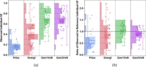
Figure 4. (a) Average observed IUF and J2841 IUF; (b) Annual eVMT differences between observed and J2841 estimates. Observed IUF are vehicle weighed average definition.

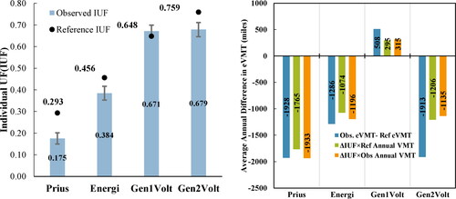
Table 4. Descriptive statistics of observed IUF.

PHEV	Mean	Std. Dev	Std. Err mean	95% C.I Mean [Lower, Upper]	Inter quartile range	Median	Median absolute deviation
Prius	0.175	0.121	0.026	[0.122,0.229]	0.115	0.143	0.050
Energi	0.384	0.231	0.032	[0.320,0.449]	0.322	0.358	0.159
Gen1Volt	0.671	0.185	0.028	[0.614,0.727]	0.280	0.681	0.146
Gen2Volt	0.679	0.190	0.032	[0.614,0.743]	0.290	0.697	0.145

3.4. Procedure to explore observed IUF deviations from the reference J2841 IUF

The goal of this procedure is to investigate what aspects of driving and charging could be probable reason(s) for Obs UF deviating from the J2841 UF expectations and calculate the individual contribution of each of these sources to the total deviation in UF. Consider Equation (7)(7) $$\mathrm{UF}(R_{\mathrm{CD}})=\frac{\stackrel{\text{CD VMT }(\mathrm{eVMT})}{\overbrace{{\sum }_{k¯1}^N\min (d(k),R_{\mathrm{CD}})}}\mathrm{ }}{{\sum }_{k-1}^N\min (d(k),R_{\mathrm{CD}})+\underset{\text{CS VMT }(\mathrm{gVMT})}{\underbrace{({\sum }_{k-1}^{N}d(k)-{\sum }_{k-1}^N\min (d(k),R_{\mathrm{CD}}))}}}$$(7) which is obtained from the basic buildup of the J2841 UF shown in Equation (1)(1) $$\mathrm{UF}\left(R_{\mathrm{CD}}\right)=\frac{{\sum }_{k-1}^N\min \left(d\left(k\right),R_{\mathrm{CD}}\right)\mathrm{ }}{{\sum }_{k-1}^{N}d\left(k\right)}\mathrm{ }$$(1) by rearranging the terms and expressing the denominator as the sum of eVMT and gVMT. For the sake of brevity, Equation (7)(7) $$\mathrm{UF}(R_{\mathrm{CD}})=\frac{\stackrel{\text{CD VMT }(\mathrm{eVMT})}{\overbrace{{\sum }_{k¯1}^N\min (d(k),R_{\mathrm{CD}})}}\mathrm{ }}{{\sum }_{k-1}^N\min (d(k),R_{\mathrm{CD}})+\underset{\text{CS VMT }(\mathrm{gVMT})}{\underbrace{({\sum }_{k-1}^{N}d(k)-{\sum }_{k-1}^N\min (d(k),R_{\mathrm{CD}}))}}}$$(7) is rewritten as Equation (8)(8) $${\mathrm{UF}}_{\mathrm{ref}}\left(R_{\mathrm{CDref}}\right)=\frac{e_{\mathrm{ref}}}{v_{\mathrm{ref}}}=\frac{e_{\mathrm{ref}}}{e_{\mathrm{ref}}+g_{\mathrm{ref}}}\mathrm{ };\mathrm{ }{\mathrm{UF}}_{\mathrm{obs}}\left(R_{\mathrm{CDobs}}\right)=\frac{e_{\mathrm{obs}}}{v_{\mathrm{obs}}}=\frac{e_{\mathrm{obs}}}{e_{\mathrm{obs}}+g_{\mathrm{obs}}}\mathrm{ }$$(8) , where e,g,v denotes the annual eVMT, gVMT, and VMT and similar expression can be written for the observed PHEVs. Disparities between Obs UF and J2841 UF ($\Delta \mathrm{UF}={\mathrm{UF}}_{\mathrm{obs}}-{\mathrm{UF}}_{\mathrm{ref}}$ could be due to variations in one or more of the following: (i) Annual VMT $\left(v_{\mathrm{obs}}-v_{\mathrm{ref}}\right)$ which in turn manifests as differences in eVMT $\left(e_{\mathrm{obs}}-e_{\mathrm{ref}}\right)$ and/or gVMT $\left(g_{\mathrm{obs}}-g_{\mathrm{ref}}\right);$ (ii) charging behavior which directly impacts $\left(e_{\mathrm{obs}}-e_{\mathrm{ref}}\right);$ (iii) Daily VMT distribution which influences range utilization and thereby determines eVMT; and (iv) Observed CD range digressing from EPA label estimates$\left(R_{\mathrm{CDobs}}-R_{\mathrm{CDref}}\right).$ (7) $$\mathrm{UF}(R_{\mathrm{CD}})=\frac{\stackrel{\text{CD VMT }(\mathrm{eVMT})}{\overbrace{{\sum }_{k¯1}^N\min (d(k),R_{\mathrm{CD}})}}\mathrm{ }}{{\sum }_{k-1}^N\min (d(k),R_{\mathrm{CD}})+\underset{\text{CS VMT }(\mathrm{gVMT})}{\underbrace{({\sum }_{k-1}^{N}d(k)-{\sum }_{k-1}^N\min (d(k),R_{\mathrm{CD}}))}}}$$(7) (8) $${\mathrm{UF}}_{\mathrm{ref}}\left(R_{\mathrm{CDref}}\right)=\frac{e_{\mathrm{ref}}}{v_{\mathrm{ref}}}=\frac{e_{\mathrm{ref}}}{e_{\mathrm{ref}}+g_{\mathrm{ref}}}\mathrm{ };\mathrm{ }{\mathrm{UF}}_{\mathrm{obs}}\left(R_{\mathrm{CDobs}}\right)=\frac{e_{\mathrm{obs}}}{v_{\mathrm{obs}}}=\frac{e_{\mathrm{obs}}}{e_{\mathrm{obs}}+g_{\mathrm{obs}}}\mathrm{ }$$(8)

We break $\Delta \mathrm{UF}$ into four components to represent the individual contribution of the four aspects to $\Delta \mathrm{UF}.$ Due to the inter-relationship between driving and charging, we consider one aspect at a time, and then, include the remaining sequentially. We evaluate the effect of each of the variations individually as difference in eVMT $\left({\delta }_{\mathrm{eVMT}}\right)$ and subsequently express these in J2841 UF fraction $\left({\delta }_{\mathrm{UF}}\right)$ terms by dividing ${\delta }_{\mathrm{eVMT}}$ by $v_{\mathrm{ref}}$ as needed. To ensure parity and methodologically consistency, we have to first apply the J2841 method, Equation (1)(1) $$\mathrm{UF}\left(R_{\mathrm{CD}}\right)=\frac{{\sum }_{k-1}^N\min \left(d\left(k\right),R_{\mathrm{CD}}\right)\mathrm{ }}{{\sum }_{k-1}^{N}d\left(k\right)}\mathrm{ }$$(1) , on our dataset. Equation (9)(9) $${\mathrm{UF}}_{\mathrm{obs}}^{\mathrm{J}2841}\left(R_{\mathrm{CDobs}}\right)=\frac{e_{\mathrm{obs}}^{\mathrm{J}2841}}{e_{\mathrm{obs}}^{\mathrm{J}2841}+g_{\mathrm{obs}}^{\mathrm{J}2841}}$$(9) describes the UF, eVMT, and gVMT after applying the J2841 methodology. (9) $${\mathrm{UF}}_{\mathrm{obs}}^{\mathrm{J}2841}\left(R_{\mathrm{CDobs}}\right)=\frac{e_{\mathrm{obs}}^{\mathrm{J}2841}}{e_{\mathrm{obs}}^{\mathrm{J}2841}+g_{\mathrm{obs}}^{\mathrm{J}2841}}$$(9)

Since J2841 assumes that the travel day starts with a fully charged battery, the term $\left(e_{\mathrm{obs}}-e_{\mathrm{obs}}^{J2841}\right)$ is entirely due to charging behavior observed not aligning with the J2841 assumptions. $\left(e_{\mathrm{obs}}-e_{\mathrm{ref}}\right)$ can be rewritten as Equation (10)(10) $$\left(e_{\mathrm{obs}}-e_{\mathrm{ref}}\right)=\left(e_{\mathrm{obs}}-e_{\mathrm{obs}}^{J2841}\right)+\left(e_{\mathrm{obs}}^{J2841}-e_{\mathrm{ref}}\right)$$(10) , where $\left(e_{\mathrm{obs}}^{J2841}-e_{\mathrm{ref}}\right)$ represents the difference between Obs eVMT after applying J2841 method and Ref eVMT. The effect of charging can be further broken down based on whether the PHEVs were unable to use the full range due to inadequately charging or if the PHEVs exceeded the range capabilities by charging more and this is detailed in Subsection 4.2. This enables characterizing the net impact of charging as positive or negative depending on the magnitude of ${\delta }_{\mathrm{eVMT}}\left(\text{Inadequate Charging}\right)$ and ${\delta }_{\mathrm{eVMT}}\left(\text{Excess Charging}\right),$ Equation (11)(11) $${\mathit{\delta }}_{\mathbf{eVMT}}\left(\mathbf{Charging}\right)={-\delta }_{\mathrm{eVMT}}\left(\text{Inadequate Charging}\right)+{\delta }_{\mathrm{eVMT}}\left(\text{Excess Charging}\right) =e_{\mathrm{obs}}-e_{\mathrm{obs}}^{J2841}$$(11) . (10) $$\left(e_{\mathrm{obs}}-e_{\mathrm{ref}}\right)=\left(e_{\mathrm{obs}}-e_{\mathrm{obs}}^{J2841}\right)+\left(e_{\mathrm{obs}}^{J2841}-e_{\mathrm{ref}}\right)$$(10) (11) $${\mathit{\delta }}_{\mathbf{eVMT}}\left(\mathbf{Charging}\right)={-\delta }_{\mathrm{eVMT}}\left(\text{Inadequate Charging}\right)+{\delta }_{\mathrm{eVMT}}\left(\text{Excess Charging}\right) =e_{\mathrm{obs}}-e_{\mathrm{obs}}^{J2841}$$(11)

Next, we examine the effect of variations between Observed Daily VMT (DVMT) and Reference DVMT distributions. If the DVMT distribution is partitioned into two regions (DVMT less and more than range), charging cannot explain eVMT differences on days when DVMT exceeds the range. This is simply due to the fundamental feature of J2841 UF which assigns the minimum of range and DVMT as eVMT on that travel day and the PHEV is driven in the CS mode only after exhausting the range when DVMT exceeds range. Even if we consider the subset of days when DVMT was lower than the range, it is possible that the difference in eVMT may not be entirely captured by charging alone, i.e. $\left(e_{\mathrm{obs}}-e_{\mathrm{ref}}\right)\ne \left(e_{\mathrm{obs}}-e_{\mathrm{obs}}^{J2841}\right)$ . This is due to the differences in the DVMT distribution with respect to range. This in turn determines the fraction of range utilized on a given travel day. Therefore, the impact of variations in DVMT distribution can be scrutinized in the form of range utilized or not utilized. We present an intuitive explanation as to why the term $\left(e_{\mathrm{obs}}^{J2841}-e_{\mathrm{ref}}\right)$ captures the impact of variations in DVMT distributions.

Consider a hypothetical travel day where DVMT is less than the range and the Obs DVMT is higher (lower) than the Ref DVMT. According to the J2841 UF, the eVMT estimated using the Obs DVMT is higher (lower) compared to that of the Ref DVMT. Consider the extreme scenario where every day, all the vehicles in Obs and Ref datasets are driven at least their range. The maximum theoretical annual eVMT in this scenario $\left(e_{\max }^{J2841}\right)$ based on the J2841 UF assumptions of travel day starting with a fully charged battery every day is $365\times R_{\mathrm{CD}}$ . $\left(e_{\mathrm{obs}}^{J2841}-e_{\mathrm{ref}}\right).$ This can be rewritten as shown in Equation (12)(12) $$\begin{array}{c}{\mathit{\delta }}_{\mathbf{eVMT}}\left(\mathbf{DVMT} \mathbf{distribution} \mathbf{and} \mathbf{range} \mathbf{utilization} \right)=\left({\mathit{e}}_{\mathbf{obs}}^{\mathit{J}2841}-{\mathit{e}}_{\mathbf{ref}}\right)\\ =\left({\mathit{e}}_{\mathbf{max}}^{\mathit{J}2841}-{\mathit{e}}_{\mathbf{ref}}\right)-\left({\mathit{e}}_{\mathbf{max}}^{\mathit{J}2841}-{\mathit{e}}_{\mathbf{obs}}^{\mathit{J}2841}\right)\end{array}$$(12) by simply adding and subtracting $\left(e_{\max }^{J2841}\right)$ and rearranging the terms. (12) $$\begin{array}{c}{\mathit{\delta }}_{\mathbf{eVMT}}\left(\mathbf{DVMT} \mathbf{distribution} \mathbf{and} \mathbf{range} \mathbf{utilization} \right)=\left({\mathit{e}}_{\mathbf{obs}}^{\mathit{J}2841}-{\mathit{e}}_{\mathbf{ref}}\right)\\ =\left({\mathit{e}}_{\mathbf{max}}^{\mathit{J}2841}-{\mathit{e}}_{\mathbf{ref}}\right)-\left({\mathit{e}}_{\mathbf{max}}^{\mathit{J}2841}-{\mathit{e}}_{\mathbf{obs}}^{\mathit{J}2841}\right)\end{array}$$(12) If $\left(e_{\mathrm{obs}}^{J2841}-e_{\mathrm{ref}}\right)>0\Rightarrow \left(e_{\max }^{J2841}-e_{\mathrm{ref}}\right)>\left(e_{\max }^{J2841}-e_{\mathrm{obs}}^{J2841}\right)$ implying that $e_{\mathrm{obs}}^{J2841}$ is relatively closer in magnitude to $e_{\max }^{J2841}$ compared to $e_{\mathrm{ref}}$ resulting in better range utilization by the Obs DVMT distribution. Alternatively, the fraction of range that remains unused by the observed PHEVs is lower than that of the vehicles in the Ref DVMT distribution. This is due to the fact that compared to the NHTS (i) Obs DVMT distribution has higher share of days where DVMT was closer to or more than range; and (ii) Average DVMT observed is higher irrespective of whether DVMT was more or less than range. Converse observations are applicable if$\left(e_{\mathrm{obs}}^{J2841}-e_{\mathrm{ref}}\right)<0.$ By subtracting $\left(e_{\max }^{J2841}-e_{\mathrm{ref}}\right)\mathrm{ }$ from $\left(e_{\max }^{J2841}-e_{\mathrm{obs}}^{J2841}\right),$ we can directly estimate the effect of DVMT variations between Obs and Ref DVMT from Equation (12)(12) $$\begin{array}{c}{\mathit{\delta }}_{\mathbf{eVMT}}\left(\mathbf{DVMT} \mathbf{distribution} \mathbf{and} \mathbf{range} \mathbf{utilization} \right)=\left({\mathit{e}}_{\mathbf{obs}}^{\mathit{J}2841}-{\mathit{e}}_{\mathbf{ref}}\right)\\ =\left({\mathit{e}}_{\mathbf{max}}^{\mathit{J}2841}-{\mathit{e}}_{\mathbf{ref}}\right)-\left({\mathit{e}}_{\mathbf{max}}^{\mathit{J}2841}-{\mathit{e}}_{\mathbf{obs}}^{\mathit{J}2841}\right)\end{array}$$(12) . From a distribution perspective, $\left(e_{\mathrm{obs}}^{J2841}-e_{\mathrm{ref}}\right)$ discerns how range utilized (or not utilized) responds to the separation of distance between the two cumulative distribution function (CDF) of DVMT.

The portion of annual VMT difference that still remains to be accounted for is $\left(g_{\mathrm{obs}}-g_{\mathrm{ref}}\right)=\left(v_{\mathrm{obs}}-v_{\mathrm{ref}}\right)-\left(e_{\mathrm{obs}}-e_{\mathrm{ref}}\right).$ Equations (10)(10) $$\left(e_{\mathrm{obs}}-e_{\mathrm{ref}}\right)=\left(e_{\mathrm{obs}}-e_{\mathrm{obs}}^{J2841}\right)+\left(e_{\mathrm{obs}}^{J2841}-e_{\mathrm{ref}}\right)$$(10) and (12)(12) $$\begin{array}{c}{\mathit{\delta }}_{\mathbf{eVMT}}\left(\mathbf{DVMT} \mathbf{distribution} \mathbf{and} \mathbf{range} \mathbf{utilization} \right)=\left({\mathit{e}}_{\mathbf{obs}}^{\mathit{J}2841}-{\mathit{e}}_{\mathbf{ref}}\right)\\ =\left({\mathit{e}}_{\mathbf{max}}^{\mathit{J}2841}-{\mathit{e}}_{\mathbf{ref}}\right)-\left({\mathit{e}}_{\mathbf{max}}^{\mathit{J}2841}-{\mathit{e}}_{\mathbf{obs}}^{\mathit{J}2841}\right)\end{array}$$(12) together represent the difference in eVMT between Observed and Reference $\left(e_{\mathrm{obs}}-e_{\mathrm{ref}}\right).$ This surplus (or deficient) eVMT observed is equivalent to deficient (or surplus) gVMT in the reference travel dataset. Therefore, while examining the impact of variations in annual VMT, only the net gVMT that still has not been accounted for must be considered as shown in Equation (13)(13) $${\mathit{\delta }}_{\mathbf{gVMT}}\left(\mathbf{Annual} \mathbf{VMT}\right)=\left|v_{\mathrm{obs}}-v_{\mathrm{ref}}\right|-\left|e_{\mathrm{obs}}-e_{\mathrm{ref}}\right|$$(13) . Equation (13)(13) $${\mathit{\delta }}_{\mathbf{gVMT}}\left(\mathbf{Annual} \mathbf{VMT}\right)=\left|v_{\mathrm{obs}}-v_{\mathrm{ref}}\right|-\left|e_{\mathrm{obs}}-e_{\mathrm{ref}}\right|$$(13) forces ${\mathrm{\Delta }}_{\mathrm{gVMT}}$ to be negative in case the variations in eVMT captured by Equations (10)(10) $$\left(e_{\mathrm{obs}}-e_{\mathrm{ref}}\right)=\left(e_{\mathrm{obs}}-e_{\mathrm{obs}}^{J2841}\right)+\left(e_{\mathrm{obs}}^{J2841}-e_{\mathrm{ref}}\right)$$(10) and (12)(12) $$\begin{array}{c}{\mathit{\delta }}_{\mathbf{eVMT}}\left(\mathbf{DVMT} \mathbf{distribution} \mathbf{and} \mathbf{range} \mathbf{utilization} \right)=\left({\mathit{e}}_{\mathbf{obs}}^{\mathit{J}2841}-{\mathit{e}}_{\mathbf{ref}}\right)\\ =\left({\mathit{e}}_{\mathbf{max}}^{\mathit{J}2841}-{\mathit{e}}_{\mathbf{ref}}\right)-\left({\mathit{e}}_{\mathbf{max}}^{\mathit{J}2841}-{\mathit{e}}_{\mathbf{obs}}^{\mathit{J}2841}\right)\end{array}$$(12) subsumes the variations in total VMT so that in this case gVMT is not treated as excess gVMT observed. (13) $${\mathit{\delta }}_{\mathbf{gVMT}}\left(\mathbf{Annual} \mathbf{VMT}\right)=\left|v_{\mathrm{obs}}-v_{\mathrm{ref}}\right|-\left|e_{\mathrm{obs}}-e_{\mathrm{ref}}\right|$$(13)

Finally, we address the difference between EPA label and observed range. The label range is determined by testing the PHEV using standardized dynamometer drive cycles (U.S. Environmental Protection Agency [EPA], 2018) in accordance with the recommended practices outlined in J1711. In CD mode, electrical energy consumption is influenced by vehicle driving speed, acceleration, road network topology, and prevailing traffic conditions. If the observed PHEVs are driven more aggressively (high speeds/acceleration, higher share of highway specific driving compared to city specific driving for example) compared to the test cycles, their kWh/mile will be higher than the label kWh/mile. By aggregating the kWh consumed and the miles driven in trips where the engine was never turned on (ZE trips), we calculate the kWh/mile consumed. The average usable electrical energy per eVMT when the PHEV is operated in the CD-EV mode (ZE trips) will be used as an indicator to gauge by how much on-road and EPA label expected range differ. This quantifies the relative electrical energy efficiency, i.e., the ratio of observed kWh/mile to label kWh/mile or $\eta ,$ Equation (14)(14) $$\eta =\frac{{\left(\frac{\mathrm{kWh}}{\mathrm{mile}}\right)}_{\mathrm{obs}}}{{\left(\frac{\mathrm{kWh}}{\mathrm{mile}}\right)}_{\mathrm{ref}}}$$(14) . If $\eta >1,$ effective range is lower than label estimates by $\eta .$ Using this effective range, we recalculate the J2841 UF. The difference between the UF corresponding to effective and label estimates represents the impact of observed driving characteristics deviating from test cycle expectations. It is expressed in UF and as eVMT in Equations (15)(15) $${\mathit{\delta }}_{\mathbf{UF}}\left(\mathbf{Efficiency}\right)=\mathrm{UF}\left(R_{\mathrm{CDobs}}=\frac{R_{\mathrm{CDref}}}{\eta }\right)-\mathrm{UF}\left(R_{\mathrm{CDref}}\right);$$(15) and (16)(16) $${\delta }_{\mathrm{eVMT}}\left(\mathrm{Efficiency}\right)={\delta }_{\mathrm{UF}}\left(\mathrm{Efficiency}\right)\times v_{\mathrm{ref}}$$(16) , respectively. Although this approach is an approximation, it nevertheless provides a valuable understanding of whether the test cycles adequately reflect real-world operation and on-road energy consumption. Estimating the impact of driving conditions and style on effective range at every operating point or understanding the relationship between kWh/mile and speed or acceleration was deemed out of scope for this study, and therefore, we use this simplified form. (14) $$\eta =\frac{{\left(\frac{\mathrm{kWh}}{\mathrm{mile}}\right)}_{\mathrm{obs}}}{{\left(\frac{\mathrm{kWh}}{\mathrm{mile}}\right)}_{\mathrm{ref}}}$$(14) in ZE trips (no engine turn-on event) (15) $${\mathit{\delta }}_{\mathbf{UF}}\left(\mathbf{Efficiency}\right)=\mathrm{UF}\left(R_{\mathrm{CDobs}}=\frac{R_{\mathrm{CDref}}}{\eta }\right)-\mathrm{UF}\left(R_{\mathrm{CDref}}\right);$$(15) (16) $${\delta }_{\mathrm{eVMT}}\left(\mathrm{Efficiency}\right)={\delta }_{\mathrm{UF}}\left(\mathrm{Efficiency}\right)\times v_{\mathrm{ref}}$$(16)

The left-hand side of Equations (10)(10) $$\left(e_{\mathrm{obs}}-e_{\mathrm{ref}}\right)=\left(e_{\mathrm{obs}}-e_{\mathrm{obs}}^{J2841}\right)+\left(e_{\mathrm{obs}}^{J2841}-e_{\mathrm{ref}}\right)$$(10) , (12)(12) $$\begin{array}{c}{\mathit{\delta }}_{\mathbf{eVMT}}\left(\mathbf{DVMT} \mathbf{distribution} \mathbf{and} \mathbf{range} \mathbf{utilization} \right)=\left({\mathit{e}}_{\mathbf{obs}}^{\mathit{J}2841}-{\mathit{e}}_{\mathbf{ref}}\right)\\ =\left({\mathit{e}}_{\mathbf{max}}^{\mathit{J}2841}-{\mathit{e}}_{\mathbf{ref}}\right)-\left({\mathit{e}}_{\mathbf{max}}^{\mathit{J}2841}-{\mathit{e}}_{\mathbf{obs}}^{\mathit{J}2841}\right)\end{array}$$(12) , and (13)(13) $${\mathit{\delta }}_{\mathbf{gVMT}}\left(\mathbf{Annual} \mathbf{VMT}\right)=\left|v_{\mathrm{obs}}-v_{\mathrm{ref}}\right|-\left|e_{\mathrm{obs}}-e_{\mathrm{ref}}\right|$$(13) are divided by $v_{\mathrm{ref}},$ and then, summed with the left-hand side of Equation (16)(16) $${\delta }_{\mathrm{eVMT}}\left(\mathrm{Efficiency}\right)={\delta }_{\mathrm{UF}}\left(\mathrm{Efficiency}\right)\times v_{\mathrm{ref}}$$(16) . $\Delta \mathrm{UF}$ is the actual deviation in UF, Equation (17)(17) $$\Delta \mathbf{UF}={\mathbf{IUF}}_{\mathbf{obs}}-{\mathbf{IUF}}_{\mathbf{ref}}$$(17) . $\Delta \mathrm{UF}$ is expressed as the sum of deviations due to four aspects of driving and charging, Equation (18)(18) $$\Delta \mathbf{UF}\cong {\pm \mathit{\delta }}_{\mathbf{UF}}\left(\mathbf{Charging}\right)\pm {\mathit{\delta }}_{\mathbf{UF}}\left(\mathbf{Range} \mathbf{Utilization}\right)\pm {\mathit{\delta }}_{\mathbf{UF}}\left(\mathbf{Annual} \mathbf{VMT}\right)\pm {\mathit{\delta }}_{\mathbf{UF}}\left(\mathbf{Efficiency}\right)$$(18) . We use $\pm$ to indicate that the contribution to $\Delta \mathbf{UF}$ could be positive or negative except for annual VMT since it represents CS mode gVMT. To account for circumstances which the four factors explained above may not entirely capture, an error component to denote the unobservable factors has been included. The authors would like to draw the distinction between this error component from random errors and latent factors which varies from vehicle to vehicle. Error in the context of this methodology accounts for the remaining difference due to unobservable factors, Equation (19)(19) $$\Delta \mathbf{UF}={\pm \mathit{\delta }}_{\mathbf{UF}}\left(\mathbf{Charging}\right)\pm {\mathit{\delta }}_{\mathbf{UF}}\left(\mathbf{Range} \mathbf{Utilization}\right)\pm {\mathit{\delta }}_{\mathbf{UF}}\left(\mathbf{Annual} \mathbf{VMT}\right)\pm {\mathit{\delta }}_{\mathbf{UF}}\left(\mathbf{Efficiency}\right)\pm {\mathit{\delta }}_{\mathbf{UF}}\left(\mathbf{error}\right)$$(19) . (17) $$\Delta \mathbf{UF}={\mathbf{IUF}}_{\mathbf{obs}}-{\mathbf{IUF}}_{\mathbf{ref}}$$(17) (18) $$\Delta \mathbf{UF}\cong {\pm \mathit{\delta }}_{\mathbf{UF}}\left(\mathbf{Charging}\right)\pm {\mathit{\delta }}_{\mathbf{UF}}\left(\mathbf{Range} \mathbf{Utilization}\right)\pm {\mathit{\delta }}_{\mathbf{UF}}\left(\mathbf{Annual} \mathbf{VMT}\right)\pm {\mathit{\delta }}_{\mathbf{UF}}\left(\mathbf{Efficiency}\right)$$(18) (19) $$\Delta \mathbf{UF}={\pm \mathit{\delta }}_{\mathbf{UF}}\left(\mathbf{Charging}\right)\pm {\mathit{\delta }}_{\mathbf{UF}}\left(\mathbf{Range} \mathbf{Utilization}\right)\pm {\mathit{\delta }}_{\mathbf{UF}}\left(\mathbf{Annual} \mathbf{VMT}\right)\pm {\mathit{\delta }}_{\mathbf{UF}}\left(\mathbf{Efficiency}\right)\pm {\mathit{\delta }}_{\mathbf{UF}}\left(\mathbf{error}\right)$$(19)

The individual contribution, ${\delta }_{\mathrm{UF}}\left(.\right)$ to $\Delta \mathbf{UF}$ is expressed as a percentage of total absolute deviation as shown in Equation (20)(20) $${\mathbf{\delta }}_{\mathbf{UF}}\left(.\right) \mathbf{\%}= \frac{{\delta }_{\mathrm{UF}}\left(.\right)}{\left|{\delta }_{\mathrm{UF}}\left(\text{Observed Factors}\right)\right|+\left|{\delta }_{\mathrm{UF}}\left(\mathrm{error}\right)\right|}$$(20) . To check the accuracy of the procedure, we calculated IUF estimated by the procedure$\left({\mathrm{IUF}}_{\mathrm{obs}.\mathrm{est}}\right)$ according to Equation (21)(21) $${\mathrm{IUF}}_{\mathrm{est}}={\mathrm{IUF}}_{\mathrm{ref}}-\Delta \mathrm{UF}$$(21) , compared it with the actual observed IUF $\left({\mathrm{IUF}}_{\mathrm{obs}.\mathrm{actual}}\right)$ and express the percentage error as shown in Equation (22)(22) $$\% \mathrm{Error}=\frac{\left({\mathrm{IUF}}_{\mathrm{obs}.\mathrm{actual}}-{\mathrm{IUF}}_{\mathrm{obs}.\mathrm{est}}\right)}{{\mathrm{IUF}}_{(.)}}\mathrm{ };\mathrm{where}\mathrm{ }\left(.\right)\in \left\{\mathrm{Ref},\mathrm{ }\mathrm{Obs},\mathrm{ }\mathrm{Est}\right\}$$(22) . (20) $${\mathbf{\delta }}_{\mathbf{UF}}\left(.\right) \mathbf{\%}= \frac{{\delta }_{\mathrm{UF}}\left(.\right)}{\left|{\delta }_{\mathrm{UF}}\left(\text{Observed Factors}\right)\right|+\left|{\delta }_{\mathrm{UF}}\left(\mathrm{error}\right)\right|}$$(20) where $\left|{\delta }_{\mathrm{UF}}\left(\text{Observed Factors}\right)\right|=\left|{\delta }_{\mathrm{UF}}\left(\mathrm{Charging}\right)\right|+\left|{\delta }_{\mathrm{UF}}\left(\text{Range Utilization}\right)\right|+\left|{\delta }_{\mathrm{UF}}\left(\text{Annual VMT}\right)\right|+\left|{\delta }_{\mathrm{UF}}\left(\mathrm{Efficiency}\right)\right|$ (21) $${\mathrm{IUF}}_{\mathrm{est}}={\mathrm{IUF}}_{\mathrm{ref}}-\Delta \mathrm{UF}$$(21) (22) $$\% \mathrm{Error}=\frac{\left({\mathrm{IUF}}_{\mathrm{obs}.\mathrm{actual}}-{\mathrm{IUF}}_{\mathrm{obs}.\mathrm{est}}\right)}{{\mathrm{IUF}}_{(.)}}\mathrm{ };\mathrm{where}\mathrm{ }\left(.\right)\in \left\{\mathrm{Ref},\mathrm{ }\mathrm{Obs},\mathrm{ }\mathrm{Est}\right\}$$(22)

4. Results

In this section, we describe the consequences of implementing the procedure outlined in Subsection 3.4 using the driving and charging data collected from the 153 PHEVs. First, we performed tests for statistically significant differences between the UF of observed PHEVs and the SAE J2841 reference estimates. Second, we apply the J2841 UF method on the observed data and discuss the impact of charging. We, then, investigate how daily VMT distribution influences range utilization. Relationship between annual VMT, charging frequency and UF is analyzed followed by a comparison between observed and label expected range and fuel economy. We synthesize our findings using the functional form represented in Equations (19)–(22) in the concluding part of this section.

4.1. Tests for statistical significance

Observed IUF and FUF of all PHEVs except Gen 1 Volt is lower than their respective Reference UF estimates, Tables 2 and 3. Although at an aggregate fleet and average vehicle level, there are differences between the Observed UF and Reference J2841 estimates, we want to ascertain if these differences are statistically significant and merit examining in detail. This was accomplished by comparing the UF (sample) of every vehicle in the dataset with the J2841 FUF and J2841 IUF (population) using t-tests and equivalence tests.

We first performed two-tailed one sample t-tests between the UF of every vehicle in the dataset with the J2841 IUF and J2841 FUF. The null hypothesis if rejected indicates that the sample Obs UF value is not equal to the hypothesized population means. At 5% significance level, the null hypothesis test of J2841 IUF was rejected for the Prius, Energi, and Gen2 Volt. Null hypothesis test for the J2841 FUF was rejected for the Prius and Gen1 Volt. We then checked if the Obs UF is within a certain interval around the population means. To perform the equivalence tests, suitable upper and lower equivalence bounds need to be specified based on the smallest effect of interest. The null hypothesis is the existence of a true effect that is at least the chosen lower or upper equivalence bound and the alternative hypothesis is that the effect falls within the chosen equivalence bound or the absence of any worthwhile effect (Lakens, 2017). To determine the effect size, we used standardized differences between the two means, namely Cohen’s d and selected the small effect size of 0.2 (Lakens, 2013; Sullivan & Feinn, 2012). The equivalence bound is the product of d and the sample standard deviation. Analysis indicated that the observed IUF and FUF of all the four PHEV models are not equivalent to the J2841 IUF and J2841 FUF at 5% significance level, respectively. The results of the t-tests and equivalence tests are summarized in Tables A6–A9 in Appendix. Using G*power (Faul et al., 2007), post hoc effect size and achieved statistical power for the sample size in our dataset was calculated and summarized in Table A10 in Appendix. We have included the FUF only as a guide and for the purpose of carrying out the statistical tests. Throughout the reminder the rest of the article, we consider the multiday (MDIUF) for analyzing UF discrepancies. Unless otherwise explicitly specified, UF and IUF refer to the MDIUF.

Table 5. Kolmogorov–Smirnov two-sample test report^a.

	KS test statistic	D = Max|F1-F2|	Observed CDF at D	NHTS CDF at D	Observed DVMT at D	Prob > D
Prius	0.058	0.152	0.264	0.416	20	<.0001*
Energi	0.0638	0.137	0.429	0.567	30	<.0001*
Gen1Volt	0.056	0.125	0.389	0.508	26	<.0001*
Gen2Volt	0.043	0.099	0.203	0.303	14	<.0001*

* Statistically significant at 5%. p <.0001* rejects null hypothesis that the two samples were drawn from the same distribution.

^a Table A12 in Appendix presents additional details including the test report for the two alternative one-sided hypothesis tests.

Table 6. Relationship between average annualized VMT, charging sessions, UF, and eVMT.

	N vehicles		VMT		eVMT		gVMT
	Below 15,000	Above 15,000	Below 15,000	Above 15,000	Below 15,000	Above 15,000	Below 15,000	Above 15,000
Prius	9	13	9597	21,165	2444	2483	7153	18,682
Energi	24	28	11,204	21,422	5232	5831	5972	15,591
Gen1Volt	21	22	10,727	21,107	8236	12,218	2491	8890
Gen2Volt	25	11	12,052	18,806	8338	12,050	3714	6756
	Observed IUF		Reference IUF		Charging sessions/driving day		ΔeVMT (Obs-Ref)
	Below 15,000	Above 15,000	Below 15,000	Above 15,000	Below 15,000	Above 15,000	Below 15,000	Above 15,000
Prius	0.255	0.117	0.293		1.47	1.24	–1951	–1912
Energi	0.467	0.272	0.456		1.69	1.69	–1608	–1009
Gen1 Volt	0.768	0.579	0.648		1.47	1.69	–1484	2497
Gen2 Volt	0.692	0.641	0.759		1.06	1.28	–3047	665

Table 7. Distribution of the contribution to IUF deviations.

	Inadequate charging	Excess charging	Range utilization	ZE trip efficiency	Annual VMT
Prius	–46.6% ± 6.7%	4.6% ± 2.3%	–20.2% ± 1.6%	–12.5% ± 8.6%	16.0% ± 15.1%
Energi	–42.5% ± 6.4%	22.0% ± 5.3%	–16.1% ± 3.1%	–7.4% ± 9.0%	–11.9% ± 13.6%
Gen1Volt	–20.1% ± 8.5%	47.1% ± 13.7%	3.2% ± 15.7%	–4.4% ± 4.3%	–25.2% ± 28.9%
Gen2Volt	–43.4% ± 8.5%	3.2% ± 2.0%	–7.0% ± 11.2%	–21.0% ± 6.7%	25.4% ± 13.3%

Mean and standard error.

Values are Means ± standard errors in italics.

4.2. Effect of charging

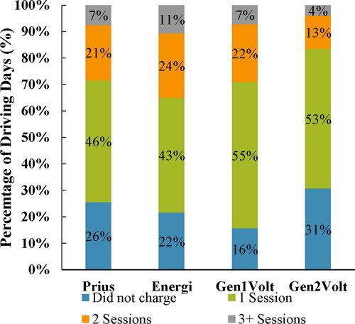
For each of the four PHEV models, we applied the J2841 method on our dataset and generated the UF curves. Figure 5 depicts these UF curves alongside the J2841 IUF (solid black line) and J2841 FUF (dashed black line) curves. Referring to Figure 6, we can see that except for the Gen1 Volt, the IUF increased by varying degrees. The increase in IUF was highest for Gen2Volt followed Prius and Energi. Figure 7 shows the percentage share of driving days by the number of charging sessions. We can see that on roughly 20%–35% of driving days, the PHEVs charged more than once and on 15%–30% of the driving days, the vehicles were not charged at all, both of these situations are not included in the J2841 UF.

Figure 5. Comparison of J2841 UF curves (truncated) generated using NHTS/J2841 estimates and observed PHEVs.

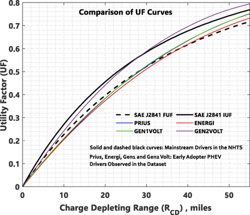
Figure 6. Means and std. error of Observed IUF, observed IUF after applying J2841 UF method, and reference J2841 IUF. Observed IUF are vehicle weighed average of UF by the definition of IUF.

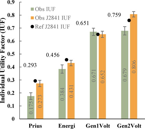
Figure 7. Percentage share of driving days by number of charging sessions.

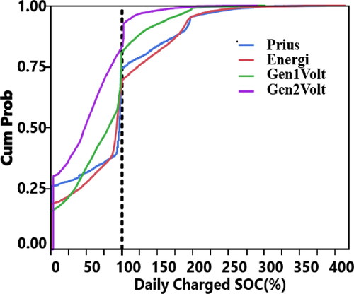
Referring to Figure 8, which shows the CDF of battery SOC at the beginning of travel day, on approximately 25% of driving days Prius and Energi started their travel on nearly empty battery (less than 5% SOC remaining indicated by the vertical dashed line in Figure 8), which also contradicts with the J2841 assumptions. The other charging related aspect not captured in J2841 UF is the possibility of PHEVs extending their CD mode of operation beyond their range by charging more than 100% of SOC. Figure 9 shows the CDF of daily charged SOC. On approximately 10%–30% of days, PHEVs either charged more than 100% or did not charge at all depending on the range.

Figure 8. CDF plot of travel day starting SOC.

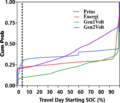
Figure 9. CDF plot daily charged SOC.

At a daily level, we calculated the difference between the observed daily eVMT and the expected J2841 eVMT. We analyzed the effect of charging by categorizing the travel day into three types: (i) PHEVs inadequately charging when Daily VMT (DVMT) is less than range; (ii) charging when DVMT exceeds range; and (iii) PHEVs exceeding their range capability by charging more than 100% SOC. The effect of charging on δeVMT is shown in Figure 10. We categorized the travel day into three types to illustrate how charging behavior influences δeVMT with respect to range. Gen1 Volts overcompensates for the eVMT missed due to not charging adequately by regaining eVMT beyond their range by charging more than 100% of SOC.

Figure 10. Effect of charging on average annualized δeVMT.

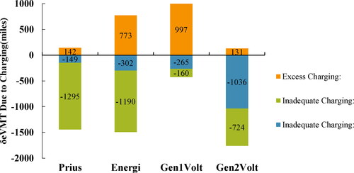
The effect of charging is most pronounced in the case of short-range PHEVs (Prius and Energi) followed by Gen2 Volts. The eVMT missed due to inadequate charging and eVMT gained by charging more frequently by Gen2 Volt reduced appreciably compared to Gen1 Volt.

4.3. Daily VMT distribution’s influence on range utilization

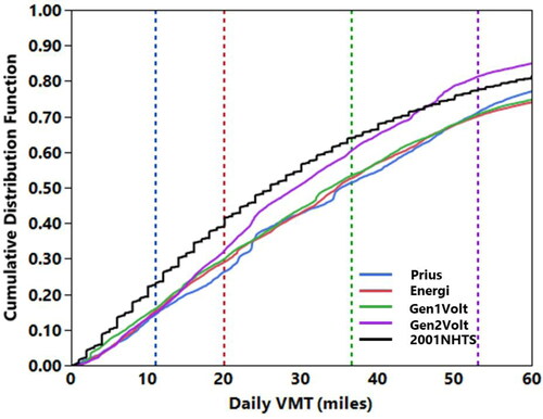
Variations in DVMT distribution between our data and NHTS expectations corresponds to variations in range utilization. Additional descriptive details of the distributions are summarized in Table A11 of Appendix. To examine this further, we compared the CDF of DVMT of observed PHEVs with the NHTS using the two-sample Kolmogorov–Simonov (KS) test. The KS test report is presented in Table A12 of Appendix. The KS test statistic D measures the maximum absolute deviation between the two CDFs. Of interest is the DVMT at which maximum deviation between the NHTS and observed PHEV CDF occurs in relation to the range.

Referring to Table 5, the observed DVMT at which maximum deviation (D) increases with range (up to Gen1 Volt) and then reduces. The maximum deviation for Gen1 and Gen2 Volts happens when DVMT is lower than their range −26 miles and 14 miles, respectively. In the case of Prius and Energi, D occurs at a value of DVMT that is 10 miles more than their range. For the Prius and Energi, the D statistic indicates that the observed PHEVs have a higher share of DVMT beyond their range. This is most noticeable for the Prius as evidenced by the value of NHTS CDF (0.416) and observed CDF at D (0.264), which is near the first quartile. For the Energi and Gen1 Volt this occurs closer to the median and in the case of Gen2 Volt, it is below the first quartile.

From Table A11, we can see that the 10%, 25%, 50%, 75%, 90% quantile DVMT of NHTS is lower than those of the observed PHEVs, except for the 75% and 90% quantile DVMT of Gen2 Volt. The mean is higher than the median across all PHEV, indicative of the left-skewed nature of the distributions. However, their extent of separation displays a gradually decreasing trend with increasing range demonstrating that the left-tail of observed PHEVs being much longer than NHTS. This effect is measured using the expression in Equation (12)(12) $$\begin{array}{c}{\mathit{\delta }}_{\mathbf{eVMT}}\left(\mathbf{DVMT} \mathbf{distribution} \mathbf{and} \mathbf{range} \mathbf{utilization} \right)=\left({\mathit{e}}_{\mathbf{obs}}^{\mathit{J}2841}-{\mathit{e}}_{\mathbf{ref}}\right)\\ =\left({\mathit{e}}_{\mathbf{max}}^{\mathit{J}2841}-{\mathit{e}}_{\mathbf{ref}}\right)-\left({\mathit{e}}_{\mathbf{max}}^{\mathit{J}2841}-{\mathit{e}}_{\mathbf{obs}}^{\mathit{J}2841}\right)\end{array}$$(12) . Referring to Figure 11, the CDF of NHTS lies entirely above the CDF of observed PHEVs up to approximately 45 miles. We can observe that the J2841 UF based on the NHTS under-represents the number of days DVMT was higher than the range of all PHEVs except Gen2 Volt. In the case of Gen2 Volt, the NHTS over-represents share of days beginning approximately 10 miles below its range. This explains why the IUF of Gen2 Volt increased the most compared to the other PHEVs when the J2841 UF method was applied, Figure 5. Expanded cumulative distribution and probability density function plots of DVMT are depicted in Figures A2 and A3 respectively in Appendix.

Figure 11. Comparison of daily VMT CDF (truncated) between NHTS and observed PHEVs.

4.4. Interactions between annual VMT, charging sessions and IUF

Calculating the net gVMT portion of annual VMT variation between observed and NHTS due to differences in range utilization or charging behavior is a straightforward task, Equation (13)(13) $${\mathit{\delta }}_{\mathbf{gVMT}}\left(\mathbf{Annual} \mathbf{VMT}\right)=\left|v_{\mathrm{obs}}-v_{\mathrm{ref}}\right|-\left|e_{\mathrm{obs}}-e_{\mathrm{ref}}\right|$$(13) . We examine the relationships between annual VMT, UF, eVMT, and charging. Table 6 summarizes the average annualized VMT, eVMT, and UF of the observed PHEVs grouped based on whether Observed annual VMT was more (or less) than Reference annual VMT (15,000 miles). Overall, 48% of observed PHEVs (74 out of 153) drove longer than 15,000 VMT. Approximately 60% of Prius, 54% of Energi, 51% of Gen1 Volt, and 31% of Gen2 Volt drove more than 15,000 miles annually. Referring to Table 6, we can see that UF reduces as the total VMT increases, since the UF is a ratio of eVMT to total VMT. If we look at ΔeVMT of Prius and Gen2 Volt that drove less than Reference annual VMT (15,000), their observed IUF was still less than the J2841 IUF.

Increase in the annual VMT traveled is associated with increase in charging frequency of all PHEVs except the Prius and Energi. Table 6 shows that the IUF of Gen1 Volt being slightly more than the J2841 UF is stemming from the group that drove more than 15,000 miles. In the case of Gen1 Volt, although charging contributes to IUF slightly exceeding J2841 IUF, the effect of range utilization also plays an equally important role. Referring to Figure 10, the additional eVMT beyond its range gained by Gen1 Volt was the highest, followed by the Energi, Prius, and Gen2 Volt. On an absolute eVMT basis, Gen2 Volt missed more eVMT by charging inadequately on days when the daily VMT was less than its range compared to the eVMT missed on days when daily VMT exceeded its range than all other PHEV models (Figure 10). If we consider ΔeVMT of short-range PHEVs (Prius and Energi), it is worthwhile to note that lower annual VMT was associated with slightly higher (Prius) or relatively comparable (Energi) frequency of charging when compared to the group that drove more than 15,000 miles annually.

The average annual VMT across the entire dataset of 153 PHEVs is 7% more (15,868 miles) than the EPA label reference 15,000 miles. We selected 15,000 miles as the cutoff based on the EPA fuel economy label assumption (U.S. EPA, 2006) but in general annual mileage depends on a variety of aspects such as built environment characteristics (land-use mix, sprawl, housing, and population densities) (Ding et al., 2017), socio-demographic attributes, typical travel needs (Chiara et al., 2019), rebound effects (Munyon et al., 2018), and charging accessibility (Chakraborty et al., 2020). In our study, the short-range PHEVs (Prius and Energi) have higher annual mileage than the longer-range PHEVs (Gen1 and Gen 2 Volts). From a directional perspective, this observed trend is consistent with evidence from nationwide studies in which the average annual VMT was estimated to be 12,400 miles, up to 20% lower than short-range PHEVs (California Air Resources Board [CARB], 2017a; Carlson, 2015). Annual VMT comparisons between this study and other PHEV observational studies are summarized in Table A13 of Appendix.

To further understand annual mileage differences between short-range and longer-range PHEVs, we compared the frequency (days/year) of long-distance travel (daily VMT 50 miles or more) and charging accessibility as they are reasonable indicators of annual mileage and IUF deviations (Chakraborty et al., 2020; Goulias et al., 2017; Plötz et al., 2018b). Prius, Energi, and Gen1 Volt had a comparable number of long-distance travel days (115 days/year), whereas Gen2 Volts were used for long-distance travel only on 78 days/year on average. Contribution of long-distance travel (100 miles or more) to annual mileage of Prius and Energi exceeded the Gen1 Volt and Gen2 Volt by roughly 3% and 6%, respectively. These are depicted in Figures A4 and A5 of Appendix. The online survey asks the respondents to specific over the past 30 days whether they charged at their home only or away from home only or both at home and away locations. We used this categorical variable for the purpose of examining the impact of charging accessibility on annual mileage and IUF. Figure A6 depicts the mean and standard error bars of annual VMT and IUF grouped by PHEV type (Prius, Energi, Gen1 Volt, Gen2 Volt) and charging accessibility (Home, Away, Home, and Away). Overall, we find that PHEVs that charged at home on average have higher annual VMT compared to the subgroup that charged at away locations and this holds true for the IUF as well (except in the case of Prius). Our analysis indicated that Energi and Volts (Gen1 and Gen2) that charged at home and away locations have the highest UF and annual VMT among their respective subgroups. We can also observe that short-range PHEVs (Prius and Energi) that charged at home and away locations on average have comparable annual mileage (17,000 miles) and the highest across the 12 groups (four PHEV types and three categories of charging accessibility).

4.5. Impact of ZE trip efficiency on effective range

To assess how efficiency of the ZE trips (kWh/mile) influences the effective range on road, we compared our results to three EPA dynamometer drive cycles that are integral to many of the performance and fuel economy standards: Urban Dynamometer Driving Schedule (UDDS), Highway Fuel Economy Test (HWFET), and Supplemental Federal Test Procedure (FTP) or US06. We express efficiency as the ratio of per-mile electrical energy consumption in ZE trips (trips where engine was never turned on) observed to the EPA label rated values. Considering the powertrain design of the Volt, which enables it to be driven as a BEV up to its range (Matthe et al., 2011), and for the purpose of not penalizing the short range PHEVs unfavorably due to their smaller range and blended mode of operation, we consider the efficiency of ZE trips alone. This is in consistent with California’s test procedures which measures the electrical energy consumed in CD-EV mode (2015).

UDDS and HWFET are intended to characterize typical urban and highway driving styles, respectively. The US06 finds its specific application to capture engine turn-on events under high speed and aggressive acceleration as part of determining the ZEV credit under California’s ZEV mandate. Figure 12(a) shows the percentage share of VMT comparison between the commonly used test cycles for fuel economy and range measurements alongside the entire fleet of PHEVs observed and NHTS by speed in mph. For the test cycles and the observed PHEVs, the distances were binned based on the actual distance driven in 5 mph speed bin intervals. For the NHTS, we used the average trip speed to bin the trip distances. Figure 12(b) compares the share of travel at different speeds between the PHEVs observed.

Figure 12. (a) Percentage share of VMT comparison between test cycles, observed PHEVs and NHTS by speed bins; (b) Percentage share of VMT comparison by speed bins.

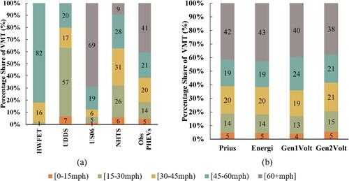
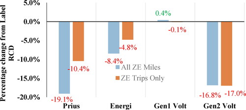
Overall, we can see that there are noteworthy differences between the test cycles and observed PHEVs, especially high speed (60+ mph) travel which neither the UDDS nor HWFET capture. If we use the average trip speed as a classifier to compare driving characteristics of NHTS vehicles with observed PHEVs, high speed travel (60 + mph) is under-represented by roughly 30%. Figure 12(b) illustrates that even among the PHEVs; there are differences in share of VMT above 45 mph. The Volts accomplish a higher share of VMT at 45–60 mph but a lower share of VMT at 60+ mph compared to the Prius and Energi. If we use 45 mph as cutoff to classify city driving (J2841 UF uses 42 mph as the threshold to obtain 55/45 city and highway driving split on the NHTS data), the city/highway driving split observed is almost 40/60. Figure 13 shows the effective range calculated. For the sake of completeness we present the effective range when we consider only the ZE trips (trips where the engine did not turn) and ZE miles which include the ZE trips and fraction of eVMT in the blended mode of operation before the first engine turn-on event. The effective range based on the energy consumption of ZE trips on average can be as low as only 83% (Gen2 Volt) of the label range or slightly more than label range (Gen1Volt).

Figure 13. Percentage difference between effective and label range.

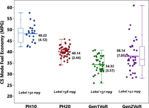
If the actual range realized on-road is less than the label expected range, the vehicle enters the CS mode after driving relatively shorter distances compared to test cycle expectations. Furthermore, due to the underrepresentation of high-speed travel in the test cycles compared to the observed share of VMT by driving speeds (Figure 12) when considered in conjunction with the observed PHEVs not realizing the label expected range on-road (Figure 13), has direct implications on the fuel economy in CS mode. On average observed CS mode fuel economy (mpg) differed from label values on average by −9% to +6%, Figure 14.

Figure 14. Distribution of observed PHEV charge sustaining mode fuel economy (mpg). Standard deviation shown within parentheses below the mean values and label values shown inset.

4.6. Consolidated effect of all observed variations

The individual effect of the four key driving and charging aspects are aggregated and depicted in Figure 15. The functional relationships between the observed IUF and the sources that contributed to its deviations from J2841 IUF were described in Subsection 3.4. The effect of charging, range utilization, annual VMT, ZE trip efficiency, and unobservable factors are expressed as percentage of total absolute deviation, Equations (17)–(20). The effect of charging is broken down into inadequate charging on both types of travel days (DVMT more and DVMT less than range) and excess charging on days when driving more than the range as explained in Subsection 4.2. With the inclusion of an error component to capture the unobservable factors, the absolute value of the percentages shown in Figure 15 sums to 100%. For clarity, the mean along with the standard errors are summarized in Table 7.

Figure 15. Combining the effect of charging behavior, range utilization, ZE trip efficiency, and annual VMT. Individual contribution is expressed as percentage of total absolute deviation, Equations (19)(19) $$\Delta \mathbf{UF}={\pm \mathit{\delta }}_{\mathbf{UF}}\left(\mathbf{Charging}\right)\pm {\mathit{\delta }}_{\mathbf{UF}}\left(\mathbf{Range} \mathbf{Utilization}\right)\pm {\mathit{\delta }}_{\mathbf{UF}}\left(\mathbf{Annual} \mathbf{VMT}\right)\pm {\mathit{\delta }}_{\mathbf{UF}}\left(\mathbf{Efficiency}\right)\pm {\mathit{\delta }}_{\mathbf{UF}}\left(\mathbf{error}\right)$$(19) and (20)(20) $${\mathbf{\delta }}_{\mathbf{UF}}\left(.\right) \mathbf{\%}= \frac{{\delta }_{\mathrm{UF}}\left(.\right)}{\left|{\delta }_{\mathrm{UF}}\left(\text{Observed Factors}\right)\right|+\left|{\delta }_{\mathrm{UF}}\left(\mathrm{error}\right)\right|}$$(20) . Percentages shown are average and the standard errors are presented in Table 7.

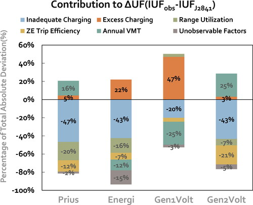
The net impact of charging is the dominant cause of Prius and Energi IUF being lower than J2841 IUF expectations even though both on average charge more than once per day, Table 1. On roughly 20%–30% of days, Prius and Energi started their travel day on a nearly empty battery, Figure 8. The second major reason is the influence of DVMT distribution on range utilization. This is mainly due to NHTS underrepresenting the share of travel accomplished on days when the Prius and Energi drove longer than their respective range. The negative impact of ZE trip mile efficiency (observed kWh/mile higher than EPA label rated kWh/mile) on Prius was slightly more compared to Energi. Despite Prius driving 1432 miles more than the reference annual VMT (15,000 miles), variations in charging and range utilization together accounted for 1928 miles of missed eVMT. In the case of Energi, there is still a portion (419 miles), of annual VMT not captured by variations in charging and range utilization. Consequently, the effect of annual VMT on Prius and Energi are displayed as positive and negative, respectively, Figure 15.

There is considerable difference in the relative contribution of the four key driving and charging aspects toward the IUF deviations from label values between the Gen1 and Gen2 Volts. Average daily charging frequency of Gen1 Volt was the highest and its IUF was slightly higher than the J2841 UF expectations. This is mainly due to the negative impact of higher annual VMT (1000 miles more than the reference annual mileage of 15,000) being almost entirely offset by the positive impact of charging more frequently. Furthermore, it is also aided in part by better range utilization and slightly better ZE trip mile efficiency. Among all PHEVs and especially within the Volts, a symbolic feature of Gen1 Volts observed in this article is their effectiveness in coordinating travel needs with charging behavior. The Gen2 Volt had the lowest annual VMT, lowest charging frequency/day and highest share of days on which it did not charge, Figure 7. The positive impact of lower annual driving was dominated by the negative effects of not charging adequately and kWh/mile of ZE trips being more than the label estimated values.

Observed charging behavior differing from the baseline single charge session per day and the travel day starting with a fully charged battery alone contributed to IUF deviating from label values of Prius and Gen2 Volts by −40% (Prius and Gen2 Volt), −21% in the case of Energi, and +27% in the case of Gen1 Volt. Differences in range utilization between NHTS and observed PHEVs were responsible for −20% to +3% of IUF deviation from J2841. Differences in annual VMT accounted for ±25% of deviation in observed IUF from J2841 UF. Observed PHEVs accomplish a higher share of VMT at speeds (45 mph or more) that is not captured by EPA certification cycles or the NHTS. Therefore, effective range of observed PHEVs realized on-road was lower than EPA label range. Variations between effective range and EPA label range influenced the IUF deviation by −20% to +1%.

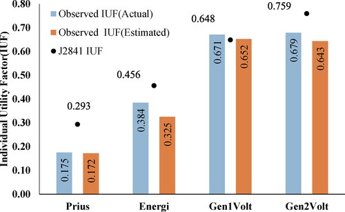
Figure 16 shows the observed IUF actual, observed IUF estimated by subtracting the deviations explained by Equation (19)(19) $$\Delta \mathbf{UF}={\pm \mathit{\delta }}_{\mathbf{UF}}\left(\mathbf{Charging}\right)\pm {\mathit{\delta }}_{\mathbf{UF}}\left(\mathbf{Range} \mathbf{Utilization}\right)\pm {\mathit{\delta }}_{\mathbf{UF}}\left(\mathbf{Annual} \mathbf{VMT}\right)\pm {\mathit{\delta }}_{\mathbf{UF}}\left(\mathbf{Efficiency}\right)\pm {\mathit{\delta }}_{\mathbf{UF}}\left(\mathbf{error}\right)$$(19) in Subsection 3.4 from the reference J2841 IUF $\left({\mathrm{IUF}}_{\mathrm{est}.}={\mathrm{IUF}}_{\mathrm{ref}}-\Delta \mathrm{UF}\right),$ and the reference J2841 IUF. We calculated the difference between the actual observed and estimated IUF. If we express this difference as a percentage of the observed IUF (actual), the procedure outlined in this article underestimates the observed IUF (actual) of Prius by 2%, Energy by 15%, Gen1 Volt by 3%, and Gen2 Volt by 5%.

Figure 16. Comparison of actual IUF and IUF estimated alongside the reference J2841 IUF. Observed IUF are vehicle weighed average of UF by the definition of IUF. Estimated and observed IUF are average values.

5. Discussion

Electrification of LDVs is essential to reduce gasoline consumption and emissions in the United States. In this regard, PHEVs continue to receive attention as an attractive vehicle technology option in the transition toward complete electrification. UF, which denotes the fraction of travel electrified, is used to measure the performance of PHEVs and is formally defined in the SAE J2841 standard. We used year-long driving and charging data of 153 PHEVs (22 Toyota Prius, 52 Ford CMax/Fusion Energi, 43 Gen 1 Volt, and 36 Gen2 Volts) with 11–53 miles of range from California, and systematically evaluated how their real-world operation deviates from the J2841 assumptions. We then quantified how each of these deviations contributes to the observed UF of PHEVs varying from their respective J2841 estimates. We elaborated on the salient traits of PHEVs observed that are not sufficiently addressed or entirely excluded from the J2841 framework in its current form.

Three charging aspects were observed that markedly differed from the J2841 UF charging assumptions of a single charging event per day and the travel day stating with a fully charged battery: (i) the tendency of PHEVs, especially those with short range (Prius and Energi) to start their travel day on an empty battery and be driven as a regular HEV; (ii) PHEVs charging on average more than once per day (except Gen2 Volt) and on roughly 15%–35% of days, PHEVs charged more than twice per day depending on the range and as a consequence; (iii) possibility for PHEVs to fully recover or even exceed their range by charging more than 100% of their SOC. This brings up an important feature missing in J2841, impact of additional charging beyond once per day on eVMT and UF and broadly speaking the value of public charging infrastructure on PHEV adoption and utilization (Ghamami et al., 2016). Although our analysis indicates that the short-range PHEVs (Prius, Energi) and Gen2 Volt missed eVMT due to not charging adequately, it could be due to contrasting reasons. In the case of short-range PHEVs, lack of sufficient incentive to maximize eVMT due to short-range, self-section bias by users who are less likely to charge or their purchase motivation was other incentives like upfront rebate, HOV lane access, and preferential parking spaces (Zhou et al., 2015). In contrast, Gen2 Volt not charging could be due to their higher range capabilities coupled with the fact that their average DVMT (39 miles) was the lowest among all the PHEVs analyzed in this article.

Prius, Energi, and Gen2 Volt are presumed to electrify a higher share of VMT according to the J2841 UF estimates compared to what they accomplished in the California sample of 153 PHEVs analyzed in this study. The characteristics (average, quantile, median, share of travel below their range, skewness, and kurtosis) of daily VMT distribution observed varied noticeably from the NHTS. When combined with the basic feature of J2841 UF which assumes that the PHEV switches to the CS mode only when daily VMT exceeds range, induced diverse impacts on IUF. Gen1 Volt had a slightly higher annual VMT, charged more on average, and has a higher IUF than the Gen2 Volt. Even though Gen2 Volt has a bigger battery and longer range, its IUF and annual eVMT was lower than that of Gen1 Volt. Moreover, the average daily VMT of Gen2 Volt (39 miles) was below its range. This could be to the misalignment between user’s driving needs and the range and/or there were other factors in play such as desire for the occasional long trips without having to charge. Marginal increase in battery capacity did improve IUF and absolute eVMT in our dataset, except in the case of Gen2 Volt.

The J2841 method presumes that all consumers utilize range equally and the marginal benefits of increasing the range is realized by all consumers in a homogenous manner. Moreover, this assumption dilutes the perception and adoption of PHEVs with varying range and drivetrain topologies in different market segments (Morton et al., 2017). This suggests that irrespective of sociodemographic indicators, potential PHEV owners are indifferent to range – meaning that their travel demand has no bearing on the range of the PHEV they eventually purchase. The NHTS draws its sample from mainstream ICE owners. Assuming travel patterns of PHEVs are identical to ICEs irrespective of range, presents an incomplete and uncertain picture of how different consumers value and utilize the same range. There is notable variation in UF for the same range (Figure 3), indicative of the fact that not all users value and utilize range homogenously. This is in stark contrast to the assumption in J2841 that users are indifferent to range which effectively decouples travel demand of potential PHEV users from the range of PHEV they eventually decide to buy.

The net environmental benefits of PHEVs depend on eVMT, which hinges on the ability of PHEVs to fully utilize their range. However, the effective range realized on the road depends on driving style (city dominant or highway dominant for example), ambient conditions, traffic, and road network topology. Our analysis indicated that the effective range realized on road was lower than the EPA label estimates for all four PHEV types. This could potentially be due to certification cycles underestimating travel at high speeds. In the medium to long-term if the trend toward high speed travel persists, it will adversely impact their life-cycle environmental and value proposition calculations. In our dataset, the share of VMT at 60 + mph by the short-range PHEVs (Prius and Energi) was higher than that of the Volts, whereas the share of travel at 45–60 mph by the Volts were higher than that of the short-range PHEVs. EPA test cycles (UDDS and HWFET) and the J2841 method of trip allocation do not reflect the city/highway style driving observed in this article across all the four PHEV types. The J2841 UF and the EPA CD test procedures are ultimately built on the hypothesis that daily VMT encapsulated in the NHTS is just a gradual extension of driving styles represented by the test cycles for range measurement (Gonder & Simpson, 2007; Liu & Santos, 2015).

A fundamental issue in evaluating the performance of PHEVs is understanding the context and experimental design under which the data was collected to estimate the UF. This is important for three reasons. First, results presented in this study clearly demonstrated that the observed PHEVs and J2841 charging and driving assumptions vary across trip, daily, and annualized timescales. It is difficult to interpret the actual performance of PHEVs calculated from data sources that are neither comparable nor compatible from a vehicle technology, time-scale, or target respondent perspectives. Second, in the case of studies that report UF from actual PHEVs, although technological capabilities are geographically neutral, ambient conditions, road network topology, travel demand, and user behavior are not. California is considered as a leader in the United States for implementing policies to mitigate the adversarial impacts of climate change concerns and has a plethora of policies that encourage PEV adoption. The performance of PHEVs observed in our analyses will be markedly different from elsewhere. Finally, apart from regional differences, as this study indicated, travel demand and charging behavior varied with range. To ensure consistency in the comparative assessment of UF with J2841 and also among the observed PHEVs, standardizing with J2841 is critical. This article developed a procedure to precisely fill this need.

5.1. PHEV policy and performance implications

The relevance of this article from demand (PHEV users) and supply (OEMs) sides, and regulatory design perspectives are described below. The article concludes with few remarks on the course of action currently being explored globally which could augment the environmental benefits of PHEVs.

The positive association between demand side purchase incentives, tax exemptions, and registration waivers, and PHEV uptake is well established across many countries. However, increasing efforts have been undertaken to ensure that they are better targeted. Currently the purchase incentives for PHEVs in California irrespective of the range (eligible PHEV models must have at least 10-mile range) is fixed at $1500. Such a mechanism does not appropriately reward longer-range PHEVs (35-miles or more) even though they have a higher UF and gasoline displacement potential than short-range PHEVs. Furthermore, behavioral aspects’ particularly charging accessibility and utilization is overlooked. This is also the case in the J2841 methodology which assumes every PHEV is charged once overnight at home and travel day starts with a fully charged battery. By extension, we can posit that the impact of intra-day charging at public charging stations and workplace on the eVMT created is ignored. This could potentially lead to perverse effects being generated in the form of missed eVMT due to not charging and used as a regular HEV, self-selection bias by users who are less likely to charge buying short-range PHEVs, or purchase was motivated by access to car-pool lanes (Tal et al., 2014). In The Netherlands and the UK, PHEVs are widely purchased as company cars for which the users get paid for fuel but not electricity is a practical example of a wrongly targeted demand side incentive that by design rewards perverse behavior (Gibbs, 2020).

One of the globally adopted strategy to promote electrified vehicles (EVs and PHEVs) is to integrate them within corporate average fuel economy and consumption standards through super credits or production multipliers and zero emission accounting provisions for the proportion of grid-electricity enabled operation (U.S. EPA, 2018; Lutsey, 2018b; Rokadiya et al., 2019; Wang et al., 2019). The UF and thereby the assumptions on charging behavior, representative driving patterns, and test cycles for range estimation are intricately linked to the broader fuel economy standards. Deviations between on-road and label UF directly influence the gap between on-road and test cycle fuel consumption of PHEVs. Observed driving and charging behavior varying from the reference and test cycles not adequately representing real-world driving patterns highlight the need for incorporating realistic driving and charging scenarios for estimating the UF. Withdrawal of several PHEV models from the market in the EU due to noncompliance under the WLTP (Emission Analytics, 2020); taking advantage of the credit multiplier and zero emissions accounting loophole that rewards short-range PHEVs in fleet fuel consumption standards by treating PHEVs as merely “compliance cars” in the United States and EU (Transport & Environment [T&E], 2018); and China’s proposed fuel economy standards that requires PHEVs to have a minimum range of 31 miles (50 km) credit qualification (ICCT, 2020) are few examples that demonstrate how regulatory mechanism and compliance flexibilities influence PHEV supply.

Looking ahead, we can foresee four major developments that could influence the performance of PHEVs from the vantage point of eVMT and UF:

• Incorporating realistic driving and charging behavior - 25% reduction in range under WLTP compared to NEDC is a tangible example that illustrates the consequences of adopting realistic test cycles for range measurement. To date no such measure has been considered to account for charging behavior deviating from the single charging session overnight at home and travel day starting on a fully charged battery. Generating UF curves by vehicle class (from compact to SUVs), annual mileage, access to charging, and recharging frequency are potential variants to consider for future PHEV UF assessments.

• Expanding OBD-II compliance requirements - Push toward remote monitoring and reporting of important in-use parameters would prevent tampering and increase the effectiveness of inspection and maintenance programs (Posada & German, 2016). California’s OBD-II regulations require reporting of blended mode and pure-EV mode eVMT and grid energy consumed, and fuel consumption in the CS mode (California OBD II Regulations, 2016). Although out of scope of this study, better understanding of PHEV engine-on events and cold-start emissions is of topical interest and one can expect an increase in such efforts – for example, Real-world Driving Emissions (RDE) test to complement SAEJ1711/WLTP to accurately measure criteria pollution using Portable Emissions Measuring Systems (Franco et al., 2019).

• OEM trends and strategies - OEMs are gradually shifting toward electrifying larger foot-print vehicles by offering PHEV versions of SUVs with bigger batteries resonating with the growing number of consumers favoring SUVs over passenger cars, especially in the U.S. Prospects for leveraging advancements in Information and Communication Technologies (ICT) through blockchain technology and geofencing capabilities are expected to improve. This serves multiple purposes from mitigating privacy and data security concerns, to accurately monitoring on-road emissions and tracking green miles traveled. This is currently being piloted in Cologne, Germany using a test fleet of 10 PHEVs (Ford, 2020). A related innovation in design is equipping the PHEVs that would automatically operate in the CD mode upon entering a low or zero-emission zone, such as the eDrive Zone project in Rotterdam, Netherlands (BMW, 2020).

• Public charging infrastructure expansion - As the share of potential PHEV owners living in apartment complexes, especially as the uptake of PHEVs increase in dense urban metros, public charging infrastructure would play a crucial role in supplementing home-charging infrastructure or lack thereof.

J2841 UF is widely used to evaluate the performance of PHEVs despite its simplistic and restrictive assumptions about how PHEVs are driven and charged. These assumptions determine how PHEVs are assessed in regulatory and incentive-based policies. The extent to which these assumptions capture real-world operation of PHEVs has a cascading effect on policy signals that inform automakers about future vehicle designs which in turn influences consumer expectations and purchase decisions. Favorable policies accompanied by improvements in battery technology and powertrain architecture, and charging infrastructure expansion, will increase the number of PHEV model offerings for prospective PHEV users. Consequently, it will be valuable to consider real-world scenarios that deviate from J2841 expectations to enhance the representativeness of UF estimates. As a step in this direction, this study examined PHEV usage and presented insights on their real-world usage. Data collection from additional PHEV models: 25-mile range Toyota Prius Prime and 32-mile Chrysler Pacifica are ongoing. Future research direction includes replicating the procedure outlined in this article to other PHEV models, understanding the impact of UF deviations from a life-cycle emissions and total cost of ownership perspectives, and quantifying the impact of public charging infrastructure on PHEV usage and eVMT.

Abbreviations
AER	=	all electric range in miles;
BEV	=	battery electric vehicle;
CAFC	=	corporate average fuel consumption;
CAFE	=	corporate average fuel economy;
CARB	=	California air resources board;
CD	=	charge depleting;
CDB	=	charge depleting blended;
CEC	=	California energy commission;
CLTC	=	China light-duty vehicle test cycle;
CS	=	charge sustaining;
CSFUF	=	city specific fleet utility factor;
CVRP	=	clean vehicle rebate project;
EER	=	energy economy ratio;
EIA	=	energy information administration;
EPA	=	environmental protection agency;
EU	=	European Union;
EV	=	electric vehicle;
eVMT	=	vehicle miles traveled on electricity;
EVSE	=	electric vehicle supply equipment;
FCT	=	full charge test;
FTP	=	federal test procedure. UDDS plus first 505 seconds of additional UDDS;
FUF	=	fleet utility factor;
GHG	=	greenhouse gases;
GPS	=	global positioning system;
gVMT	=	vehicle miles traveled on gasoline;
HEV	=	hybrid electric vehicle;
HOV	=	high occupancy vehicle;
HSFUF	=	highway specific fleet utility factor;
HWFET	=	highway fuel economy test procedure;
ICE	=	internal combustion engine vehicle;
IUCP	=	in-use confirmatory program;
IUVP	=	in-use verification program;
LCFS	=	low carbon fuel standards;
LDV	=	light duty vehicles, includes trucks and passenger cars;
MDIUF	=	multiday individual utility factor;
MPG	=	miles per gallon;
MY	=	model year;
NEDC	=	new European driving cycle;
NHTS	=	national household travel survey;
NOx	=	nitrogen oxides;
OBD	=	on board diagnostics;
OEM	=	original equipment manufacturer;
PEMS	=	portable emissions measurement system;
PEV	=	plug-in electric vehicle (PHEV and BEVs);
PHEVX	=	plug-in hybrid electric vehicle with X miles of RCD;
PM	=	particulate matter;
RCD:	=	charge depleting range in miles;
RCDA	=	actual charge depleting range in miles. Distance traveled at which the battery is completely depleted;
RCDC	=	cycle charge depleting range in miles. The total number of cycles driven at least partially in CD mode multiplied by the cycle distance for a given FCT;
RDE	=	real-world driving emissions;
SAE	=	society of automotive engineers;
SDIUF	=	single day individual utility factor;
SOC	=	state of charge (%);
SRPHEV	=	short-range PHEV. PHEV with less than 20 miles of RCD;
SUV	=	sports utility vehicle;
UDDS	=	urban dynamometer driving schedule;
UF	=	utility factor;
US:	=	United States of America;
VMT	=	vehicle miles traveled;
WLTP	=	worldwide harmonized light vehicles testing procedure;
ZEV	=	zero emission vehicle;
zVMT	=	zero emissions vehicle miles traveled. VMT on electricity alone without any engine turn-on event. Analogous to the eVMT in the CD-EV mode

Data availability statement

The data that support the findings of this study are available from the Plug-in Hybrid and Electric Vehicle Center, Institute of Transportation Studies at University of California, Davis. The Restrictions as per University of California, Davis Institutional Review Board Administration and the Institute of Transportation Studies, Davis, and the California Air Resources Board apply to the availability of these data.

Additional information

Funding

Data collected and used in this article was funded by California Air Resources Board under contract number 12-319. The authors would like to thank the California Air Resources Board and the California Energy Commission for their support. The statements and conclusions presented are those of the contractor and not necessarily those of the California Air Resources Board or the California Energy Commission. The mention of commercial products, their source, or their use in connection with material reported herein is not to be construed as actual or implied endorsement of such products.

Notes

1 On a one-to-one comparison between the PHEV models in this study and the CVRP database. This difference is due to the launch of 25-mile range Prius Prime PHEV in 2017, which was excluded when comparing the proportional shares. If we use the OEM, then the OEMs of the analyzed PHEVs in this study account for 87% of the CVRP rebates issued to PHEVs.

2 Ratio of gallons per mile (CS mode) to electrical energy consumed per mile in CD-EV mode (kWh/mile)

3 Investor owned utilities (IOUs) are Pacific Gas & Electric (PGE), San Diego Gas & Electric(SDGE), and Southern California Edison (SCE). Sacramento Municipal Utility District (SMUD) and Los Angeles Department of Water and Power (LADWP) are the two public owned utilities (POUs).

Appendix

Exponential and fit coefficients for UF estimation

Regulatory test cycles in the United States, EU, Japan, and China

Summary of UF estimates from various studies

Sampling comparisons

Tests for statistical significance

Daily VMT descriptive summaries comparisons between NHTS and Observed PHEVs

Figure A1. (Left) Percentage of PHEVs by utility company: observed and CVRP database; (Right) Percentage of PHEVs by PHEV model: observed and CVRP database.

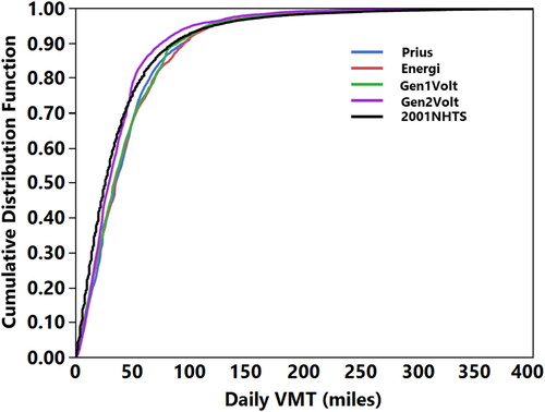
Figure A2. Expanded CDF plot of observed PHEVs and NHTS.

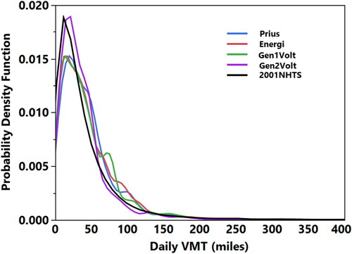
Figure A3. Expanded PDF plot of observed PHEVs and NHTS.

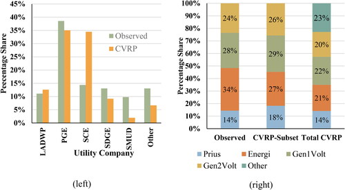
Average annual VMT and long-distance travel

Figure A4. Average number of days/year daily VMT exceeded 50, 100, 200 miles or more.

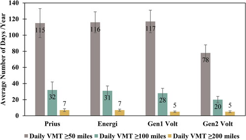
Figure A5. Share of annual VMT binned by daily VMT distance.

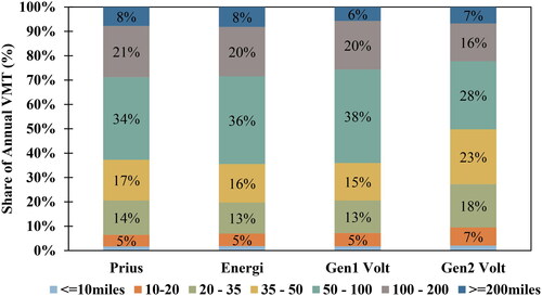
Charging accessibility, annual VMT, and observed IUF

Figure A6. Relationship between charging accessibility, annual VMT, and observed IUF. Share of PHEVs by type and charging access shown inset.

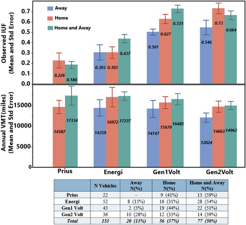
Table A1. Exponential fit coefficients for UF estimation.

	United States		South Korea	EU	Japan
Coefficient	Fleet	Individual	Fleet	Fractional	Fractional
C1	10.52	13.1	26.5	26.25	11.9
C2	–7.282	–18.7	77.9	–38.94	–32.5
C3	–26.37	5.22	–1100	–631.05	89.5
C4	79.08	8.15	2960	5964.83	–134
C5	–77.36	3.53	–1960	–25094.6	98.9
C6	26.07	–1.34		60380.21	–29.1
C7		–4.01		–87517.2	11.9
C8		–3.9		75513.77	–32.5
C9		–1.15		–35748.8	89.5
C10		3.88		7154.94	–134
Reference	(J2841, 2010)	(J2841, 2010)	(Choi et al., 2020)	(United Nations [UN], 2019)	(United Nations [UN], 2019)
Normalized distance	400 miles		600 km	800 km	400 km
Test cycles and procedures	SAE J2841 and SAE J1711		SAE J2841 and SAE J1711 (J2841, 2010; J1711, 2010)	WLTP (European Commission [EC], 2016a; 2018; Riemersma and Mock, 2017; United Nations [UN], 2019)

Table A2. Comparison of test cycle parameters used for range, fuel economy, energy and emission estimation in different regions.

Driving cycle parameters	Units	NEDC	WLTP	FTP75	HWFET	CAFE	JC08	CLTC
Country		EU (European Commission, 2016b; Kühlwein et al., 2014)		United States (U.S. Environmental Protection Agency [EPA], 2018, 2019; Kühlwein et al., 2014)			Japan (International Council on Clean Transportation [ICCT], 2019)	China (Liu et al., 2018; Wang et al., 2020)
Cycle distance	km	11	23.25	11.99	16.5		8.17	14.5
Average speed	kmph	33.6	46.5	31.5	77.7	43	24.4	29
Maximum speed	kmph	120	131	91.2	96.4		81.6	114
Cycle time	s	1180	1800	1369	765		1204	1800
Average Acceleration	ms^–Citation2	0.53	0.53	0.5	0.19	0.42	0.42	0.45
Average Deceleration	ms^–Citation2	–0.75	–0.58	–0.58	–0.22	–0.49	–0.45	–0.5
Acceleration fraction	%	20.9	30.9	39.7	44.2	40.8	35.9	28.7
Deceleration fraction	%	15.1	28.6	34.7	38.8	35.7	33.6	26.4
Cruising fraction	%	40.3	27.8	8	16.5	10.1	1.7	22.8
Idling fraction	%	23.7	13.4	17.6	0.5	13.2	28.7	22.1
Driving Style(s)		Urban, Extra Urban	4-phase^a	Urban	Highway

^a Divided into four phases(low, medium, high, and extra high) with the average speeds increasing with each subsequent phase representative of urban (up to 35 mph) , suburban (up to 47 mph), up to 60 mph, and up to 81 mph driving, respectively.

NEDC: New European driving cycle; WLTP: Worldwide harmonized light duty vehicle test procedure; FTP75: Federal test procedure. Urban Dynamometer Driving Schedule (UDDS) plus the first 505 seconds of another UDDS; HWFET: Highway fuel economy test cycle; CAFE: Corporate average fuel economy; JC08 Japanese Test Cycle up to 2020 and from 2030 onwards will be replaced by WLTP; CLTC: China Light-duty Vehicle Test Cycle. CLTC is currently under development and is expected to replace the WLTP. China currently uses modified NEDC and will use the WLTP until the transition to CLTC is complete.

Table A3. Summary of UF estimates from various studies.

PHEV model	Range (miles)^a	N vehicles	Reported UF	Label UF^b	% Deviation from label UF	Region	Data source
Chevy Gen1 Volt	35/38	1867	0.745	0.573/0.591	28.0%	United States (Smart et al., 2014)	In use data logging
Chevy Gen1 Volt	35	787	0.724	0.573	26.4%	United States (Carlson, 2015)
Chevy Gen1 Volt	38	618	0.739	0.600	23.2%
Chevy Gen1 Volt	35/38	48,000–63,000	0.74	0.573/0.591	27.1%	United States and Canada (Duhon et al., 2015)
Chevy Gen2 Volt	50	48,000–63,000	0.8	0.707	13.2%
Ford Cmax	20	5368	0.328	0.396	–17.2%	United States (Carlson, 2015)
Ford Cmax	20	10,253	0.328	0.396	–17.2%	United States (California Air Resources Board [CARB], 2017a)
Ford Fusion	20	5803	0.352	0.396	–11.1%	United States (Carlson, 2015)
Ford Fusion	20	12,842	0.343	0.396	–13.4%	United States (California Air Resources Board [CARB], 2017a)
Toyota Prius	11	1523	0.164	0.247	–33.6%	United States (California Air Resources Board [CARB], 2017a; Carlson, 2015)
Honda Accord	13	189	0.222	0.284	–21.8%
BMW i3 REX	72/80	8309	0.921	0.793/0.821	13.7%	United States (California Air Resources Board [CARB], 2017a)
Chevy Gen1 Volt	38	1831	0.785	0.591	32.8%	United States and Canada (Plötz et al., 2017)	User reported and aggregate OBD telematics data
Toyota Prius	11	88	0.304	0.247	23.1%	Germany (Plötz et al., 2017)
Opel Ampera	38	25	0.723	0.591	22.3%
Mitsubishi Outlander	23	46	0.469	0.442	6.1%
Volvo V60	24	15	0.486	0.534	–9.0%
Audi A3	31	197	0.59	0.755	–21.9%	Norway (Figenbaum and Kolbenstvedt, 2016)	Survey of existing PHEV users
Opel Ampera	52	46	0.72	0.874	–11.9%
BMW C350e	19	11	0.41	0.607	–32.5%
VW Golf GTE	31	283	0.57	0.755	–12.6%
Mitsubishi Outlander	32	806	0.55	0.766	–11.2%
Toyota Prius	16	67	0.38	0.536	–6.7%
Volvo V60	31	104	0.51	0.755	–11.3%
Opel Ampera	51	1190	0.44–0.48	0.77	–40.3%	Netherlands (van Gijlswijk and Ligterink, 2018)	In use data logging
Chevrolet Volt	51	203	0.44–0.49	0.77	–40.3%
Toyota Prius	15	906	0.15–0.19	0.5	–66.0%
Volvo V60	31	2738	0.23–0.3	0.67	–61.2%
Mitsubishi Outlander	32	5390	0.29–0.35	0.68	–52.9%
Ford Cmax	20	229	0.28–0.37	0.64	–48.4%
Audi e-tron	31	1345	0.21–0.34	0.67	–58.2%
VW Golf GTE	31	2235	0.21–0.3	0.66	–63.6%
VW Passat GTE	31	698	0.3	0.67	–55.2%
MercedesC 350e	19	895	0.25–0.4	0.55	–40.0%
BMW i3	72/80	86	0.84–0.89	0.86	0.0%

^a Range refers to charge depleting range estimated under region specific test cycles and procedures.

^b Germany, Norway, and Netherlands Range and Label UF based on NEDC. United States and Canada Range and UF based on U.S. EPA combined city/highway UF.

Table A6. t-Test results - Comparing UF of every vehicle observed with J2841 IUF.

${\mathbf{UF}}_{\mathbf{obs}} \mathbf{and} {\mathbf{IUF}}_{\mathbf{ref}}$	t test test statistic	Prob > |t|	Prob < t	Prob > t
Prius	–4.547	0.0002	<.0001	1.000
Energi	–2.237	0.030	0.015	0.985
Gen1Volt	0.695	0.491	0.755	0.245
Gen2Volt	–2.538	0.016	0.008	0.992
p-values significant at 5% are shown in italics

Table A7. t-Test results- Comparing UF of every vehicle observed with J2841 FUF.

${\mathbf{UF}}_{\mathbf{obs}}\mathrm{ }\mathbf{and}\mathrm{ }{\mathbf{FUF}}_{\mathbf{ref}}$	t test test statistic	Prob > |t|	Prob < t	Prob > t
Prius	–2.769	0.012	0.006	0.994
Energi	–0.394	0.696	0.348	0.652
Gen1Volt	2.944	0.0053	0.997	0.0026
Gen2Volt	–0.897	0.376	0.188	0.812
p-values significant at 5% are shown in italics

Table A8. Equivalence tests- Comparing UF of every vehicle observed with J2841 IUF.

	Equivalence region	${\mathit{H}}_0:\mathrm{ }{\mathbf{UF}}_{\mathbf{obs}}\le {\mathbf{IUF}}_{\mathbf{ref}}-\mathbf{\Delta }$		${\mathit{H}}_0:\mathrm{ }{\mathbf{UF}}_{\mathbf{obs}}\ge {\mathbf{IUF}}_{\mathbf{ref}}+\mathbf{\Delta }$
		t-Ratio	p-Value	t-Ratio	p-Value
Prius	[0.269,0.317]	–3.620	.999	–5.475	<.0001
Energi	[0.410,0.502]	–0.800	.786	–3.673	.000
Gen1Volt	[0.614,0.688]	2.02	.024	0.605	.274
Gen2Volt	[0.721,0.797]	–1.339	.905	–3.738	.0003
α = 0.05, $\mathrm{\Delta }=0.2\mathrm{ }\left({\mathrm{Cohen}}^{\mathrm{\text{'}}}\mathrm{s}\mathrm{ }d\right)\times \text{sample Std}.\mathrm{Dev}.$

Table A9. Equivalence tests- comparing UF of vehicle observed with J2841 FUF.

	Equivalence region	${\mathit{H}}_0:\mathrm{ }{\mathbf{UF}}_{\mathbf{obs}}\le {\mathbf{FUF}}_{\mathbf{ref}}-\mathbf{\Delta }$		${\mathit{H}}_0:\mathrm{ }{\mathbf{UF}}_{\mathbf{obs}}\ge {\mathbf{FUF}}_{\mathbf{ref}}+\mathbf{\Delta }$
		t-Ratio	p-Value	t-Ratio	p-Value
Prius	[0.223,0.271]	–1.842	.960	–3.697	.001
Energi	[0.351,0.443]	1.043	.151	–1.830	.037
Gen1Volt	[0.551,0.625]	4.257	<.0001	1.631	.945
Gen2Volt	[0.669,0.745]	0.303	.382	–2.096	.022
α = 0.05, $\mathrm{\Delta }=0.2\mathrm{ }\left({\mathrm{Cohen}}^{\mathrm{\text{'}}}\mathrm{s}\mathrm{ }d\right)\times \text{sample Std}.\mathrm{Dev}.$

Table A10. Post hoc two-tailed t tests achieved power and effect size for given α and sample size.

	Observed IUF and J2841 IUF		Observed IUF and J2841 FUF
	Power (1-β)	Effect size d	Power (1-β err prob)	Effect size d
Prius	0.992	0.975	0.947	0.801
Energi	0.597	0.312	0.512	0.281
Gen1Volt	0.109	0.1111	0.463	0.291
Gen2Volt	0.690	0.421	0.44	0.189
α = 0.05, Effect size d = 0.2 (small), d = 0.5(medium), d = 0.8 Large

Table A11. NHTS and observed PHEVs: DVMT descriptive statistics.

	Quantiles
	10	25	50	75	90	Mean
NHTS	5	12	26	50	85.5	40
Prius	8.7	19.2	35.2	56.9	94.7	46
Energi	8.3	16.9	34.7	61.7	95.4	46
Gen1Volt	7.1	16.2	33.8	60.6	88.6	44
Gen2Volt	7.8	16.0	29.3	47.8	75.4	39
	Median absolute deviation	Skewness	Kurtosis	Lower 95% Mean	Upper 95% Mean	IQR
NHTS	16	5.2	52.0	39.5	40.7	38.0
Prius	18	3.9	28.1	44.7	46.8	37.7
Energi	20	3.8	26.3	45.5	47.0	44.8
Gen1Volt	20	2.8	14.5	43.7	45.1	44.4
Gen2Volt	15	5.1	48.5	38.2	39.7	31.8

Table A12. KS test report: Comparing CDF of DVMT between NHTS and observed PHEVs.

	KS	D =Max|F1-F2|	NHTS CDF at D	Observed DVMT at D	Prob >D
Prius	0.058	0.152	0.416	20	<.0001*
Energi	0.0638	0.137	0.567	30	<.0001*
Gen1Volt	0.056	0.125	0.508	26	<.0001*
Gen2Volt	0.043	0.099	0.303	14	<.0001*
	KSa	D+ =Max(F1-F2)	Prob > D+	D-=Max(F2-F1)	Prob > D-
Prius	11.42	0.0069	0.578	0.1519	<.0001*
Energi	13.72	0.0057	0.520	0.1376	<.0001*
Gen1Volt	11.85	0.0086	0.2678	0.1250	<.0001*
Gen2Volt	8.92	0.0427	<.0001*	0.0999	<.0001*

Table A4. Comparison between observed PHEVs and Clean Vehicle Rebate Project (CVRP) database by utility company and PHEV model.

Observed PHEVs (this study)
Utility	Observed PHEVs		Prius	Energi	Gen1Volt	Gen2Volt
LADWP	17		2	5	4	6
PGE	59		11	16	17	15
SCE	22		2	7	6	7
SDGE	20		3	9	5	3
SMUD	15		1	7	6	1
Other	20		3	8	5	4
Total	153		22	52	43	36
Number of rebates issued under the CVRP 2012–2018 (Center for Sustainable Energy (CSE) and California Air Resources Board [CARB], 2019)
Utility^3	CVRP Subset^a	Total CVRP	Prius	Energi	Gen1Volt	Gen2Volt
LADWP	11,278	13,688	1569	2212	4021	3476
PGE	5848	7607	1028	1417	1695	1708
SCE	30,922	39,550	5499	8306	8746	8371
SDGE	29,911	39,711	6429	8242	8496	6744
SMUD	7803	10,409	1217	2861	1999	1726
Other	1661	2343	251	580	404	426
Total	87,423	113,308	15,993	23,618	25,361	22,451
^aSubset of CVRP includes the rebates issued to the PHEV models analyzed in this study: Toyota Plug-in Prius, Ford CMax and Fusion Energi, Gen1 Chevrolet Volt (MY 2011–2015), and Gen2 Chevrolet Volt (MY 2016 onwards). Total CVRP rebates include rebates issued to all PHEV models between 2012 and 2018.

Table A5. Sociodemographic attributes comparisons between the 2017 NHTS California Add-on (Transportation Secure Data Center, 2019) and this study.

Household ownership	Own	Rent	Gender	Male	Female
NHTS-CA	18,436(71%)	7444(29%)	NHTS-CA	26,554(48%)	29,180(52%)
This Study	122(80%)	30(20%)	This Study	106(69%)	44(29%)
Educational attainment	Less than a high school graduate	High school graduate or GED	Some college or associates degree	Bachelor’s degree	Graduate or professional degree
NHTS-CA	10,204(18%)	7391(13%)	15,043(27%)	11,837(21%)	11,282(20%)
This Study			18(12%)	49(32%)	86(56%)
Income	Less than $50,000	$50,000 to $99,999	$1,00,000 to $1,49,999	$1,50,000 to $1,99,999	$2,00,000 and more
NHTS-CA	9260(37%)	7541(30%)	4495(18%)	1844(7%)	2169(9%)
This Study	11(7%)	33(22%)	33(22%)	31(20%)	43(28%)
Household size	1	2	3	4	5+
NHTS-CA	8459(32%)	10,928(42%)	3218(12%)	2320(9%)	1187(5%)
This Study	19(12%)	63(41%)	29(19%)	29(19%)	12(8%)
Number of drivers	0	1	2	3	4+
NHTS-CA	935(4%)	9755(37%)	12,971(50%)	1855(7%)	596(2%)
This Study		23(15%)	109(71%)	14(9%)	6(4%)

Table A13. Average annual VMT reported in literature.

	This study	EV project (Carlson, 2015)	CARB (California Air Resources Board [CARB], 2017a)	Voltstats (Plötz et al., 2018)	MyFord Mobile (Boston and Werthman, 2016)
Prius	16,432	15,136	15,283	12,694
Energi	16,705	12,403	13,920/15,076		12,674/14,058
Gen1 Volt	16,038	12,238	12,403	8517–10,828
Gen2 Volt	14,115

References

- Aviquzzaman, M. (2014). Analysis of plug-in hybrid electric vehicles' utility factors using gps-based longitudinal travel data. Lamar University-Beaumont.
- Björnsson, L.-H., & Karlsson, S. (2017). Electrification of the two-car household: PHEV or BEV? Transportation Research Part C: Emerging Technologies, 85, 363–376.
- Björnsson, L.-H., Karlsson, S., & Sprei, F. (2018). Objective functions for plug-in hybrid electric vehicle battery range optimization and possible effects on the vehicle fleet. Transportation Research Part C: Emerging Technologies, 86, 655–669.
- BMW. (2020). BMW E-drive Zones – Automatically emission-free in the city. Retrieved May 5, from https://www.bmwgroup.com/en/company/bmw-group-news/artikel/bmw-edrive-zones.html
- Boston, D., & Werthman, A. (2016). Plug-in vehicle behaviors: An analysis of charging and driving behavior of ford plug-in electric vehicles in the real world. World Electric Vehicle Journal, 8(4), 926–935.
- Bradley, T. H., & Davis, B. M. (2011). Alternative plug in hybrid electric vehicle utility factor. Technical Paper, 0148-7191. Society of Automotive Engineers (SAE).
- Bradley, T. H., & Frank, A. A. (2009). Design, demonstrations and sustainability impact assessments for plug-in hybrid electric vehicles. Renewable and Sustainable Energy Reviews, 13(1), 115–128.
- Bradley, T. H., & Quinn, C. W. (2010). Analysis of plug-in hybrid electric vehicle utility factors. Journal of Power Sources, 195(16), 5399–5408.
- California Air Resources Board (CARB). (2017a). California's advanced clean cars midterm review, appendix G: Plug-in electric vehicle in-use and charging data analysis. Retrieved May 1, 2019, from https://ww2.arb.ca.gov/resources/documents/2017-midterm-review-report,
- California Air Resources Board (CARB). (2017b). California's advanced clean cars midterm review: Summary report for the technical analysis of the light duty vehicle standards. Retrieved January 10, 2019, from https://ww2.arb.ca.gov/resources/documents/2017-midterm-review-report
- California OBD II Regulations, Final Rulemaking, California Code of Regulations Sections 1968.2, 1968.5,1900, 1956.8,1971.1, 2485 of Title 13, and Sections 95302 and 95662 of Title 17, C. A. R. Board (CARB) 1968.2, 1968.5,1900, 1956.8,1971.1, and 2485. (2016).
- Carlson, B. (2015). Electric vehicle mile traveled (eVMT): On-road results and analysis. U.S. Department of Energy Vehicle Technologies Office 2015 Annual Merit Review and Peer Evaluation Meeting, June 8–11, Idaho National Laboratory, Washington, DC.
- Center for Sustainable Energy (CSE) & California Air Resources Board (CARB). (2019). Clean Vehicle Rebate Project (CVRP) Rebate Statistics. Retrieved October 15, from https://cleanvehiclerebate.org/eng/rebate-statistics
- CFR § 86.1866-12. (2018). CO 2 credits for advanced technology vehicles. U.S. Environmental Protection Agency (EPA).
- CFR § 600.116-12. (2019). Title 40 - Protection of Environment. Fuel Economy and Greenhouse Gas Exhaust Emissions of Motor Vehicles. Special procedures related to electric vehicles and hybrid electric vehicles. Chapter I, Subchapter Q, Part 600. U. S. EPA Regulatory Information.
- Chakraborty, D., Hardman, S., & Tal, G. (2020). Why do some consumers not charge their plug-in hybrid vehicles? Evidence from Californian plug-in hybrid owners. Environmental Research Letters, 15(8), 084031.
- Chiara, B. D., Deflorio, F., Pellicelli, M., Castello, L., & Eid, M. (2019). Perspectives on electrification for the automotive sector: A critical review of average daily distances by light-duty vehicles, required range, and economic outcomes. Sustainability, 11(20), 5784–5735.
- Choi, W., Yoo, E., Seol, E., Kim, M., & Song, H. H. (2020). Greenhouse gas emissions of conventional and alternative vehicles: Predictions based on energy policy analysis in South Korea. Applied Energy, 265, 114754. https://doi.org/https://doi.org/10.1016/j.apenergy.2020.114754
- Cordera, R., dell'Olio, L., Ibeas, A., & Ortúzar, J. d D. (2019). Demand for environmentally friendly vehicles: A review and new evidence. International Journal of Sustainable Transportation, 13(3), 210–223. https://doi.org/https://doi.org/10.1080/15568318.2018.1459969
- Crain, T., Gorgia, T., & Alley, R. J. (2016). Application of PHEV Fractional Utility Factor Weighting to EcoCAR On-Road Emissions and Energy Consumption Testing. Technical Paper, 0148-7191. Society of Automotive Engineers (SAE)
- Davies, J., & Kurani, K. (2010). Recharging behavior of households' plug-in hybrid electric vehicles: Observed variation in use of conversions of 5-kW-h blended plug-in hybrid electric vehicle. Transportation Research Record: Journal of the Transportation Research Board, 2191(1), 75–83. https://doi.org/https://doi.org/10.3141/2191-10
- Davies, J., & Kurani, K. S. (2013). Moving from assumption to observation: Implications for energy and emissions impacts of plug-in hybrid electric vehicles. Energy Policy, 62, 550–560.
- Ding, C., Liu, C., Zhang, Y., Yang, J., & Wang, Y. (2017). Investigating the impacts of built environment on vehicle miles traveled and energy consumption: Differences between commuting and non-commuting trips. Cities, 68, 25–36.
- Duhon, A. N., Sevel, K. S., Tarnowsky, S. A., & Savagian, P. J. (2015). Chevrolet volt electric utilization. SAE International Journal of Alternative Powertrains, 4(2), 269–276.
- Duoba, M., & Bocci, D. (2009). Calculating results and performance parameters for PHEVs. Technical Paper, 0148-7191. Society of Automotive Engineers (SAE).
- Elango, V. V., Guensler, R., & Ogle, J. (2007). Day-to-day travel variability in the Commute Atlanta, Georgia, study. Transportation Research Record: Journal of the Transportation Research Board, 2014(1), 39–49. https://doi.org/https://doi.org/10.3141/2014-06
- Emission Analytics. (2020). Plug-in hybrids without behavioural compliance risk failure. Tensions between official EU emissions policy and member states. Retrieved April 10, from https://www.emissionsanalytics.com/news/2020/1/8/plug-in-hybrids-without-behavioural-compliance-risk-failure
- European Automobile Manufacturers’ Association (ACEA). (2017). The worldwide harmonised light-duty vehicle test procedure (WLTP) facts. Retrieved March 30, 2020, from https://www.wltpfacts.eu/wltp-benefits/
- European Commission (EC). (2014). Proposal for an Electric Vehicle Regulatory Reference Guide Submitted by the Working Party on Pollution and Energy in accordance with the programme of work of the Inland Transport Committee for 2012–2016 (ECE/TRANS/224, para. 94 and ECE/TRANS/2012/12, programme activity 02.4) for consideration and endorsements by WP.29. Retrieved February 1, 2020, from https://www.unece.org/fileadmin/DAM/trans/doc/2014/wp29/ECE-TRANS-WP29-2014-81e.pdf
- European Commission (EC). (2016a). Technical Report on the development of a Worldwide Harmonised Light duty vehicle Test Procedure (WLTP). European Commission, Brussels. Retrieved February 10, 2020, from https://circabc.europa.eu/sd/a/a19b42c8-8e87-4b24-a78b-9b70760f82a9/July%202018%20Technical%20Guidelines.pdf
- European Commission. (2016b). Technical Report on the development of a Worldwide Harmonised Light duty vehicle Test Procedure (WLTP). UN/ECE/WP.29/GRPE/WLTP-IG. Retrieved February 15, 2020, from https://www.unece.org/fileadmin/DAM/trans/doc/2015/wp29grpe/GRPE-72-02.pdf
- European Commission (EC). (2017). Commission Recommendation of 31.5.2017: On the use of fuel consumption and CO2 emission values type-approved and measured in accordance with the World Harmonised Light Vehicles Test Procedure when making information available for consumers pursuant to Directive 1999/94/EC of the European Parliament and of the Council. Retrieved March 30, 2020, from https://ec.europa.eu/transport/sites/transport/files/c20173525-recommendation-wltp.pdf
- European Commission. (2018). Technical Guidelines for the preparation of applications for the approval of innovative technologies pursuant to Regulation (EC) No 443/2009 and Regulation (EU) No 510/2011.
- Faul, F., Erdfelder, E., Lang, A.-G., & Buchner, A. (2007). G*Power 3: A flexible statistical power analysis program for the social, behavioral, and biomedical sciences. Behavior Research Methods, 39(2), 175–191. https://doi.org/https://doi.org/10.3758/bf03193146
- Figenbaum, E., & Kolbenstvedt, M. (2016). Learning from Norwegian battery electric and plug-in hybrid vehicle users: Results from a survey of vehicle owners. In TØI report, 8248017184. Retrieved March 15, 2020, from https://www.toi.no/getfile.php?mmfileid=43161
- Figenbaum, E., & Weber, C. (2018). Estimating real-world emissions of PHEVs in Norway by combining laboratory measurement with user surveys. World Electric Vehicle Journal, 9(2), 31.
- FleetCarma. (2019). C2 and C5 logger specifications. https://www.fleetcarma.com/documents/. Retrieved January 1.
- Ford. (2020). Blockchain trial brings hybrid-drive Transits to Cologne. Retrieved May 1. https://fordeurope.blogspot.com/2019/10/blockchain-trial-brings-hybrid-drive.html
- Francfort, J. (2014). 2014 DOE vehicle technologies office review - EV project data & analytic results. Idaho National Laboratory (INL). Retrieved May 10, 2019, from https://energy.gov/sites/prod/files/2014/07/f18/vss137_francfort_2014_o.pdf
- Franco, P. V. J., Suarez-Bertoa, R., Astorga, C., Clairotte, M., Giechaskiel, B., Valverde, V., & Kregar, Z. (2019). On-road vehicle emissions beyond RDE conditions: Experimental assessment addressing EU Real-Driving Emission (RDE). Joint Research Centre (European Commission) Technical Report. KJ-NA-29905-EN-N.
- Fuel Economy Labeling of Motor Vehicles: Revisions To Improve Calculation of Fuel Economy Estimates; Final Rule. Docket Number EPA-HQ-OAR-2005-0169. (2006). U.S. EPA 40 CFR Parts 86 and 400.
- General Motors (GM). (2016). 2016 Chevrolet Volt Battery System. Retrieved March 20, 2020, form https://media.gm.com/content/dam/Media/microsites/product/Volt_2016/doc/VOLT_BATTERY.pdf
- Ghamami, M., Nie, Y., & Zockaie, A. (2016). Planning charging infrastructure for plug-in electric vehicles in city centers. International Journal of Sustainable Transportation, 10(4), 343–353.
- Gibbs, N. (2020). Plug-in hybrids give automakers an emissions compliance lifeline, 2019. Retrieved April 20, from https://europe.autonews.com/automakers/plug-hybrids-give-automakers-emissions-compliance-lifeline
- Goebel, D., & Plötz, P. (2019). Machine learning estimates of plug-in hybrid electric vehicle utility factors. Transportation Research Part D: Transport and Environment, 72, 36–46.
- Gonder, J., Markel, T., Thornton, M., & Simpson, A. (2007). Using global positioning system travel data to assess real-world energy use of plug-in hybrid electric vehicles. Transportation Research Record: Journal of the Transportation Research Board, 2017(1), 26–32. https://doi.org/https://doi.org/10.3141/2017-04
- Gonder, J., & Simpson, A. (2007). Measuring and reporting fuel economy of plug-in hybrid electric vehicles. World Electric Vehicle Journal, 1(1), 134–141.
- Goulias, K., Davis, A., Elizabeth, M. C., Janowicz, K., & Zhou, R. (2017). Long Distance Travel in the California Household Travel Survey. Final Report Contract Number: 64A0529 Task Order: 047. UC Santa Barbara, Caltrans, and UCConnect. Retrieved April 10, 2020, from http://ucconnect.berkeley.edu/sites/default/files/file_uploads/2016-TO-047-65A0529.pdf
- Grahn, P., Alvehag, K., & Soder, L. (2014). PHEV utilization model considering type-of-trip and recharging flexibility. IEEE Transactions on Smart Grid, 5(1), 139–148.
- Hao, X., Zhou, Y., Wang, H., & Ouyang, M. (2020). Plug-in electric vehicles in China and the USA: A technology and market comparison. Mitigation and Adaptation Strategies for Global Change, 25(3), 325–329.
- Hardman, S., Plotz, P., Tal, G., Axsen, J., Figenbaum, E., Karlsson, S., Refa, N., Sprei, F., Williams, B., Whitehead, J. & Witkamp, B. (2019). Exploring the role of plug-in hybrid electric vehicles in electrifying passenger transportation. Research Report UCD-ITS-RR-19-01.
- Hu, P. S., & Reuscher, T. R. (2004). Summary of travel trends: 2001 national household travel survey. Retrieved March 1, 2019, from https://nhts.ornl.gov/2001/pub/STT.pdf
- International Council on Clean Transportation (ICCT). (2019). Japan 2030 fuel economy standards, policy update. Retrieved December 10, 2019, from https://theicct.org/sites/default/files/publications/Japan_2030_standards_update_20190927.pdf
- J1711_201006. (2010) Recommended practice for measuring the exhaust emissions and fuel economy of hybrid-electric vehicles, including plug-in hybrid vehicles. Society of Automotive Engineers (SAE).
- J1772_201710. (2017). Electric vehicle and plug in hybrid electric vehicle conductive charge coupler. Society of Automotive Engineers (SAE).
- J2841_201009. (2010). Utility factor definitions for plug-in hybrid electric vehicles using travel survey data. Society of Automotive Engineers (SAE).
- Johnson, C., & Williams, B. (2017). Characterizing plug-in hybrid electric vehicle consumers most influenced by california’s electric vehicle rebate. Transportation Research Record: Journal of the Transportation Research Board, 2628(1), 23–31. https://doi.org/https://doi.org/10.3141/2628-03
- Karabasoglu, O., & Michalek, J. (2013). Influence of driving patterns on life cycle cost and emissions of hybrid and plug-in electric vehicle powertrains. Energy Policy, 60, 445–461.
- Kühlwein, J., German, J., & Bandivadekar, A. (2014). Development of test cycle conversion factors among worldwide light-duty vehicle CO2 emission standards. The International Council on Clean Transportation(ICCT) White Paper. Retrieved July 10, 2019, from https://theicct.org/sites/default/files/publications/ICCT_LDV-test-cycle-conversion-factors_sept2014.pdf
- Lakens, D. (2013). Calculating and reporting effect sizes to facilitate cumulative science: A practical primer for t-tests and ANOVAs. Frontiers in Psychology, 4, 863. https://doi.org/https://doi.org/10.3389/fpsyg.2013.00863
- Lakens, D. (2017). Equivalence tests: A practical primer for t tests, correlations, and meta-analyses. Social Psychological and Personality Science, 8(4), 355–362. https://doi.org/https://doi.org/10.1177/1948550617697177
- Lee, T.-K., Adornato, B., & Filipi, Z. S. (2011). Synthesis of real-world driving cycles and their use for estimating PHEV energy consumption and charging opportunities: Case study for Midwest/US. IEEE Transactions on Vehicular Technology, 60(9), 4153–4163.
- Liao, F., Molin, E., & van Wee, B. (2017). Consumer preferences for electric vehicles: A literature review. Transport Reviews, 37(3), 252–275.
- Ligterink, N. E., van Mensch, P., Cuelenaere, R. F. A. (2016). NEDC - WLTP comparative testing, Dutch Ministry of Infrastructure and the Environment, TNO Report 2016 R11285. Retrieved March 10, 2020, from https://publications.tno.nl/publication/34622355/ZCzWY2/TNO-2016-R11285.pdf
- Liu, J., & Santos, G. (2015). Plug-in hybrid electric vehicles’ potential for urban transport in china: The role of energy sources and utility factors. International Journal of Sustainable Transportation, 9(2), 145–157.
- Liu, Y., Zhou, H., Xu, Y., Kongjian, Q., & Yu, H. (2018). Feasibility study of using WLTC for fuel consumption certification of chinese light-duty vehicles. Technical Paper, 0148-7191. Society of Automotive Engineers(SAE).
- Lutsey, N. (2018a). California's continued electric vehicle market development. International Council on Clean Transportation. Retrieved July 2, 2018, from https://www.theicct.org/sites/default/files/publications/CA-cityEV-Briefing-20180507.pdf
- Lutsey, N. (2018b). Integrating electric vehicles within U.S. and European efficiency regulations. Working Paper 2017-07. The International Council on Clean Transportation(ICCT).
- Lutsey, N., Meszler, D., Isenstadt, A., German, J., & Miller, J. (2017, March 22) Efficiency technology and cost assessment for US 2025–2030 light-duty vehicles. White Paper. International Council on Clean Transportation (ICCT), Washington, USA.
- Matthe, R., Turner, L., & Mettlach, H. (2011). VOLTEC battery system for electric vehicle with extended range. SAE International Journal of Engines, 4(1), 1944–1962.
- Morton, C., Anable, J., & Nelson, J. D. (2017). Consumer structure in the emerging market for electric vehicles: Identifying market segments using cluster analysis. International Journal of Sustainable Transportation, 11(6), 443–459.
- Munyon, V. V., Bowen, W. M., & Holcombe, J. (2018). Vehicle fuel economy and vehicle miles traveled: An empirical investigation of Jevon’s Paradox. Energy Research & Social Science, 38, 19–27.
- Neubauer, J., Brooker, A., & Wood, E. (2013). Sensitivity of plug-in hybrid electric vehicle economics to drive patterns, electric range, energy management, and charge strategies. Journal of Power Sources, 236, 357–364.
- Neubauer, J., & Wood, E. (2014). Thru-life impacts of driver aggression, climate, cabin thermal management, and battery thermal management on battery electric vehicle utility. Journal of Power Sources, 259, 262–275.
- Paffumi, E., Gennaro, M. D., & Martini, G. (2018). Alternative utility factor versus the SAE J2841 standard method for PHEV and BEV applications. Transport Policy, 68, 80–97.
- Plötz, P., Funke, S., & Jochem, P. (2015). Real-world fuel economy and CO2 emissions of plug-in hybrid electric vehicles. Working Paper Sustainability and Innovation.
- Plötz, P., Funke, S. Á., & Jochem, P. (2018a). Empirical fuel consumption and CO2 emissions of plug‐in hybrid electric vehicles. Journal of Industrial Ecology, 22(4), 773–784.
- Plötz, P., Funke, S. Á., & Jochem, P. (2018b). The impact of daily and annual driving on fuel economy and CO2 emissions of plug-in hybrid electric vehicles. Transportation Research Part A: Policy and Practice, 118, 331–340.
- Plötz, P., Funke, S., Jochem, P., & Wietschel, M. (2017). CO 2 mitigation potential of plug-in hybrid electric vehicles larger than expected. Scientific Reports, 7(1), 16493. https://doi.org/https://doi.org/10.1038/s41598-017-16684-9
- Posada, F., & German, J. (2016). Review of LDV OBD requirements under the European, Korean and Californian emission programs. The International Council on Clean Transportation (ICCT) White Paper.
- Poullikkas, A. (2015). Sustainable options for electric vehicle technologies. Renewable and Sustainable Energy Reviews, 41, 1277–1287.
- Riemersma, I., & Mock, P. (2017). Too low to be true? How to measure fuel consumption and CO2 emissions of plug-in hybrid vehicles, today and in the future. Briefing. Retrieved January 15, 2019, from https://www.theicct.org/sites/default/files/publications/EU-PHEV_ICCT-Briefing-Paper_280717_vF.pdf
- Rokadiya, S., Yang, Z., & Bandivadekar, A. (2019). Incentivizing Electric Vehicles to Meet Fuel Consumption Standards for Passenger Cars in India. The International Council on Clean Transportation (ICCT) White Paper.
- Searle, S., Pavlenko, N., & Lutsey, N. (2016). Leading edge of electric vehicle market development in the United States: An analysis of California cities. International Council on Clean Transportation.
- Section 1962.2. (2015). Title 13, California Code of Regulations (CCR). California exhaust emission standards and test procedures for 2018 and subsequent model zero-emission vehicles and hybrid electric vehicles, in the passenger car, light-duty truck and medium-duty vehicle classes.
- Smart, J., Bradley, T., & Salisbury, S. (2014). Actual versus estimated utility factor of a large set of privately owned Chevrolet Volts. SAE International Journal of Alternative Powertrains, 3(1), 30–35.
- Smart, J., Powell, W., & Schey, S. (2013). Extended range electric vehicle driving and charging behavior observed early in the EV project. Technical Paper, 0148-7191. Society of Automotive Engineers (SAE).
- Smart, J., Shirk, M., Kurani, K., Quinn, C., & Davies, J. (2010). Electricity demand of PHEVs operated by private households and commercial fleets: Effects of driving and charging behavior. 25th World Battery, Hybrid, and Fuel Cell Electric Vehicle Symposium & Exhibition, Shenzhen, China.
- Sullivan, G. M., & Feinn, R. (2012). Using effect size-or why the P value is not enough. Journal of Graduate Medical Education, 4(3), 279–282. https://doi.org/https://doi.org/10.4300/JGME-D-12-00156.1
- Tal, G. (2020). Advanced plug-in electric vehicle travel and charging behavior -final report. California Air Resources Board Contract #12-319 (Under Review), Report 2020.
- Tal, G., Nicholas, M. A., Davies, J., & Woodjack, J. (2014). Charging behavior impacts on electric vehicle miles traveled: Who is not plugging in? Transportation Research Record: Journal of the Transportation Research Board, 2454(1), 53–60. https://doi.org/https://doi.org/10.3141/2454-07
- Tamor, M. A., Gearhart, C., & Soto, C. (2013). A statistical approach to estimating acceptance of electric vehicles and electrification of personal transportation. Transportation Research Part C: Emerging Technologies, 26, 125–134.
- The International Council on Clean Transportation (ICCT). (2020). Comments on China's proposed 2021-2025 fuel consumption limits, evaluation methods, and targets for passenger cars. Retrieved May 1, from https://theicct.org/news/comments-chinas-proposed-2021-2025-fuel-consumption-limits-evaluation-methods-and-targets
- Transport & Environment (T&E). (2018). EU cars CO2 regulation and plug-in hybrid cars. European Federation for Transport and Environment AISBL, Policy Briefing. Retrieved April 2, 2020, from https://www.transportenvironment.org/sites/te/files/publications/Cars%20CO2%20PHEV%20analysis.pdf
- Transportation Secure Data Center. (2019). 2017 National Household Travel Survey – California Add-On. National Renewable Energy Laboratory. Retrieved January 15, from https://www.nrel.gov/transportation/secure-transportation-data/tsdc-nhts-california.html
- Turrentine, T., & Tal, G. (2015). Advanced plug-in electric vehicle usage and charging behavior. Contract #12-319. CARB and CEC.
- U.S. Environmental Protection Agency (EPA). (2018). Dynamometer Drive Schedules. Retrieved December 1, from https://www.epa.gov/vehicle-and-fuel-emissions-testing/dynamometer-drive-schedules
- U.S. Environmental Protection Agency (EPA). (2019a). Inventory of U. S. Greenhouse Gas Emissions and Sinks: 1990-2017, April 11, EPA 430-R-19-001. https://www.epa.gov/ghgemissions/inventory-us-greenhouse-gas-emissions-and-sinks-1990-2017
- U.S. Environmental Protection Agency (EPA). (2019b). Fuel economy data. Retrieved January 1, form https://www.fueleconomy.gov/feg/download.shtml
- United Nations (UN). (2019). United Nations Global Technical Regulation (GTR) on the Evaporative emission test procedure for the Worldwide harmonized Light vehicles Test Procedure (WLTP EVAP). United Nations, Brussels, ECE/TRANS/180/Add.15/Amend.5. Retrieved February 10, 2020, from https://www.unece.org/fileadmin/DAM/trans/main/wp29/wp29r-1998agr-rules/GTR15-am5-For_Registry_EN.pdf
- van Gijlswijk, R., & Ligterink, N. E. (2018). Real-world fuel consumption of passenger cars based on monitoring of Dutch fuel pass data 2017. TNO Report 2018 R10371. Den Haag: TNO.
- Wang, J., Liu, C., Ton, D., Zhou, Y., Kim, J., & Vyas, A. (2011). Impact of plug-in hybrid electric vehicles on power systems with demand response and wind power. Energy Policy, 39(7), 4016–4021.
- Wang, S., Chen, K., Zhao, F., & Hao, H. (2019). Technology pathways for complying with Corporate Average Fuel Consumption regulations up to 2030: A case study of China. Applied Energy, 241, 257–277.
- Wang, Y., Hui, C., & Liu, Y. (2020). Research on the test and evaluation method of fuel consumption based on chinese light-duty test cycle. Technical Paper, 0148-7191. Society of Automotive Engineers (SAE).
- Wood, E. W., Rames, C. L., Bedir, A., Crisostomo, N., & Allen, J. (2018) California plug-in electric vehicle infrastructure projections: 2017-2025-Future infrastructure needs for reaching the state's zero emission-vehicle deployment goals. National Renewable Energy Lab. (NREL), Golden, CO (United States), 17-ALT-01; TN # 224505. Retrieved March 1, 2019, form https://www.nrel.gov/docs/fy18osti/70893.pdf
- Wu, X., Aviquzzaman, M., & Lin, Z. (2015). Analysis of plug-in hybrid electric vehicles’ utility factors using GPS-based longitudinal travel data. Transportation Research Part C: Emerging Technologies, 57, 1–12.
- Zhou, Y., Levin, T., & Plotkin, S. E. (2016). Plug-in Electric Vehicle Policy Effectiveness: Literature Review. Argonne National Laboratory. U.S. Department of Energy Office of Energy Policy and Systems Analysis.
- Zhou, Y., Wang, M., Hao, H., Johnson, L., Wang, H., & Hao, H. (2015). Plug-in electric vehicle market penetration and incentives: A global review. Mitigation and Adaptation Strategies for Global Change, 20(5), 777–795.