Analyzing the city-level effects of land use on travel time and CO₂ emissions: a global mediation study of travel time

Abstract

This global study simultaneously analyzes how land use differences between cities affect travel time and CO₂ emissions. The land use–travel time–carbon emission relationship in which the time is specified as a mediator is analyzed at the city level on an international scale based on individually reported data by moving away from the tendency of conducting country-level, regional-scale analysis based on estimates from travel survey data or satellite images. A major finding of the structural equation model is that because of the high population density in their high-density built-up areas, compact developments with urban cores reduce travel, and indirectly lessen CO₂ emissions (complete mediation by travel time). In contrast, despite no effect on travel, gross population density in the entire city is found to have a direct effect in reducing per-capita emissions based partially on the economies of scale. The proportion of the low-density built-up area in the city also directly reduces the emissions, which might reinforce the concept of the paradox of intensification. Among the control variables, household size, fuel price, and congestion level may ultimately lead to less CO₂ emissions because their direct effects, which are positive on travel time, would be overwhelmed by the negative effects on CO₂ emissions.

Keywords:

• Carbon emissions
• land use
• mediating effects
• structural equation modeling
• travel time

1. Introduction

Research on how land use affects travel has an over 60-year history, beginning with Mitchell and Rapkin’s book (Mitchell & Rapkin, 1954), Urban Traffic: A Function of Land Use, and Levinson and Wynn’s research article (Levinson & Wynn, 1963), which was published in the second issue of Highway Research Record. Particularly, the article suggested that high population density in the neighborhood is significantly related to fewer automobile trips. Such an effort has gradually confirmed—at least regarding the statistical significance, but not the magnitude—at the metropolitan and regional levels, how land use variations in a neighborhood have effects on travel behavior and energy consumption (Cao & Fan, 2012; Ewing et al., 2008), but how the variations between cities exert effects at the international level is still an unanswered question (Gim, 2012; Giuliano & Dargay, 2006) despite continuous attempts (e.g., Kenworthy & Laube, 1999; Newman & Kenworthy, 1989b; Schwanen, 2002).

Due to high external (in)validity/transferability, however, international-scale research is frequently cited. As an iconic image in the transportation field, Newman and Kenworthy charted an inversely proportional (exponentially negative) relationship that gross population density has with per-capita automobile use and subsequent energy use. This relationship has been referred to by thousands of research articles, textbooks, and policy reports (Ewing et al., 2018). To confirm/correct the chart, this study aims to analyze the effects of land use variables including gross population density on travel.

Specifically, the purpose of this study is twofold: (1) to simultaneously analyze land use effects on travel and carbon dioxide (CO₂) emissions through one model (Holz-Rau & Scheiner, 2019) in which travel is specified as a mediator/intermediary in the land use–carbon emission relationship and (2) to analyze the data of land use, travel, and carbon emissions at the city level (Sovacool & Brown, 2010) on a global scale (Bechle et al., 2011; Rahman, 2017). The remainder of the paper is organized as follows. First, the literature is reviewed to describe how this study differs from previous studies. Then, it presents the methodology employed for city-level research on a global scale. Empirical results are provided in the order of the bivariate correlation between land use and travel/carbon emissions, the direct effect of land use, and its indirect effect (or the mediating effect of travel). The paper ends with a summary of the findings and their implications.

2. Literature review

In the following two subsections, this study will separately review previous research on the relationship that land use has with travel behavior and air quality. Regarding the land use–travel relationship, it will show the importance of inferential studies based on appropriate statistical controls. Then, studies on the land use–air quality relationship will be reviewed in terms of data availability and accuracy. This study will accordingly justify the analysis of travel behavior as a mediator of the land use–air quality relationship.

2.1. The land use–travel relationship

This subsection presents a review of aggregate (city-level) studies on an international scale that analyzed the relationship between density-based land use variables and travel or carbon emissions. In this sense, studies conducted in a single country—for example, a book by Ewing et al. (2008), Growing Cooler—is not reviewed. Why the review is limited to city-level aggregate studies is that intrinsically, they have different interests from a currently predominant approach in the literature, which is individual-level disaggregate studies, and the difference typically brings about different results on the density–travel relationship (Ewing et al., 2018; Handy, 2005). According to Ewing et al. (2018), disaggregate studies evaluate the density in the immediate neighborhood while controlling for the characteristics of the entire city (e.g., in the same sprawling city, how commuting from pedestrian-friendly and automobile-oriented neighborhoods differ), whereas aggregate studies are interested in variations in city-level variables and their effects (e.g., how living in sprawling and compact cities differentiates travel patterns). Generally, individuals’ travel is affected by city-level characteristics rather than neighborhood variables (Ewing et al., 2018).¹ Similarly, based on a review of 30 Nordic studies on the land use–travel relationship, Naess (2012) reported that while previous studies often focused on micro-scale land use variables, travel tends to be affected mainly by land use characteristics relative to the city-level structure such as the population density of a continuous urban area. This tendency is particularly so with regard not to walking/biking, but to motorized travel, which is more directly related to fossil energy use and carbon emissions (Gim, 2017); whether to use the automobile hinges on distances to urban centers rather than those to local facilities. In fact, studies have found that variations in the spatial unit in which density is evaluated differentiate the density–travel relationship (Boarnet & Crane, 2001; Buchanan et al., 2006; Sultana & Weber, 2007).

Among the pioneers of global comparisons across cities/metropolitan areas, Newman and Kenworthy’s book (Newman & Kenworthy, 1989a) and research article (Newman & Kenworthy, 1989b) analyzed 32 metropolitan areas and argued that gross population density is most strongly related to energy consumption by automobile travel. In their follow-up studies, Newman and Kenworthy (2006, 2011) reaffirmed that in global comparisons, fuel use is inversely associated with gross population density. Kenworthy and Laube’s update (Kenworthy & Laube, 1999) also expanded the sample size to 46 cities and again demonstrated a clear relationship. Based on a sample of 58 cities, Newman and Kenworthy’s most recent global study (Newman & Kenworthy, 2015) analyzed population density and additionally, transit service. They consistently found that population density is the most important in explaining per-capita automobile use (transit service was also significant, but conditional on the density).

However, because other variables on travel and energy use (e.g., wealth) were not duly controlled for (Gim, 2012) and their studies were rarely multivariate, but bivariate (Dujardin et al., 2012), a question was raised about the inference validity of the Newman and Kenworthy-type studies (Ewing et al., 2018; Snellen et al., 2002; Stead & Marshall, 2001). Indeed, in a study that used Newman and Kenworthy’s data (Newman & Kenworthy, 1989a, 1989b) and additionally controlled for socioeconomic variables (Mindali et al., 2004), the significance of the density–gas consumption relationship disappeared. Similarly, Van de Coevering and Schwanen (2006) analyzed the same (but refined) data used for Kenworthy and Laube’s study (1999) and concluded that the relationship is not as strong as previously studied. That is, since sociodemographic variables were uncontrolled for, the simple correlation studies may have produced misestimated results (Stead, 2001), likely leading to a false positive conclusion or type I error (Gim, 2012, 2013). Because of an issue with variable control, Schwanen (2002) acknowledged that his analysis of 11 cities in Europe is inherently flawed. Such an issue originates mainly from the limited availability of the data on control variables (Schwanen, 2002; Van de Coevering & Schwanen, 2006).

From a different perspective, Choi et al. (2012) constructed a sample of 44 metropolitan cities from 23 European, North and Latin American, Asian, and African countries and analyzed how population density is associated with travel patterns and transportation energy consumption. Specifically, in each country, they selected the upper 15% and lower 15% cities according to city-level GDP, and then developed scatter plots where the horizontal axis was population density and the axis of ordinates was average daily trip frequency and trip length by motorized mode, mode share of private automobiles, and annual transportation energy use per capita. By visualizing the fact that the upper and lower cities in GDP are separately grouped, the authors argued that the wealth of a city affects travel and energy consumption. However, their argument was not grounded on inferential statistics. As another difference from this particular study, which analyzes individually reported data on carbon emissions, they estimated energy use based on a formula that consisted of travel indicators such as trip length and speed.

McIntosh et al. (2014) conducted path analysis of the pooled data of per-capita VMT (vehicle miles traveled) in 26 cities for 1970, 1980, 1990, and 2000. Among the explanatory variables—year dummies and archetype dummies (the four categories included full motorization, weak center, strong center, and traffic limiting strategies) as well as transit service and urban density variables—density and transit services were found to be particularly significant. Meanwhile, the global study was somewhat geographically limited in that the 26 cities were sampled from the U.S., Europe, Canada, and Australia, which have been substantially studied.

A common feature of the above global studies is that analyses were centered on population density. Density is easy to measure and control (Forsyth et al., 2007), and almost all governments provide city-level density data (Gim, 2012). Furthermore, insomuch as other land use variables (e.g., transit proximity, street connectivity, and land use mix) are usually correlated with density, density has been selected as a substitute for these less measurable variables or because of spatial multicollinearity (Rajamani et al., 2003; Zhang, 2004). While Gim’s meta-analysis (2013) found that spatial multicollinearity is a universal phenomenon rather than applying to particular cases, density may be an intermediate (Ewing & Cervero, 2010) or proxy (Handy, 2005) for these causal elements of land use. In this vein, Ewing and Cervero (2001) did not recommend separating density effects from others when density is found to be significant. If spatial multicollinearity is universal, interventions in density as a more controllable characteristic may be an efficient way of changing individuals’ behavior (Filion et al., 2006; Gim, 2013; Holden & Norland, 2005). Therefore, this study focuses on population density while evaluating it in different forms.

2.2. The land use–air quality relationship

In contrast to the land use–travel relationship, a request for global city-level research on the land use–air quality relationship has been consistent. Actually, research has not been substantially conducted due to limited data availability (Sovacool & Brown, 2010) rather than its low validity. This is because in city-level research, travel is an aggregate of individuals’ variations (Ewing et al., 2018; Handy, 2005), but air quality is observed and managed at a spatial level—not an individual level—such as the city (i.e., an agreement between the units of observation and analysis).

Bechle et al. (2011) used Landsat satellite-derived NO₂ estimates to investigate the relationship between land use and city-level air pollution in 83 world cities. Research variables included population, contiguity (proportion of the major contiguous built-up area to the total built-up area in a city), circularity, income (World Bank GDP), and meteorological conditions (based on a dilution rate as the product of wind-speed and mixing height). In their regression model, contiguity and population had negative and positive relationships with NO₂ concentrations, respectively. Then, since contiguity and population were correlated, the positive effect of population on the concentrations was canceled out by the stronger negative effect of contiguity.

Sovacool and Brown (2010) computed partial carbon footprints based on carbon emissions from selective sectors including vehicles, buildings, industry, agriculture, and wastes for a sample of 12 metropolitan cities. They compared the footprints with the means of their respective countries. Based on a discussion on each of the 12 cases, the authors concluded that compact and dense land use, alternative transportation to automobiles, and limited income are correlated with low carbon footprints.

Ou et al. (2017) examined whether land use variables influence automobile-generated CO₂ emissions in 35 cities in China and those in developed countries (34 U.S. and 26 European metro areas and 12 Japanese and 7 South Korean cities, all of which have more than one million population). The analytical model included explanatory variables of population density, city-level GDP per capita, and registered private automobiles per thousand persons and showed that population density significantly reduces CO₂ emissions. However, the emissions were not individually observed, but estimated by a formula that used multiple travel-related variables from personal travel surveys in respective countries (the emissions were a product of mode share, trip frequency, trip length, and travel speed by private automobiles). Thus, the study could not reveal how the density exerts an effect on CO₂ emissions regardless of the travel variables.

In summary, city-level studies on the land use–travel relationship delivered somewhat mixed results and it is related to their methodological rigor (lack of statistical inference and control). While those studies on the land use–air quality relationship are few because of the limited availability of city-level data, they consistently found it to be significant. However, the studies used air quality estimates that were derived from formulae (Ou et al., 2017; Sovacool & Brown, 2010) or satellite images (Bechle et al., 2011). By contrast, this study bases its evaluation of both travel patterns and carbon emissions on individually reported data. Also, as a step forward from previous attempts that explored the direct land use–air quality relationship, it specifies travel patterns as a mediator of the relationship and simultaneously analyzes the direct and indirect land use effects.

3. Data and methods²

In this study, the emissions were evaluated using (1) individually reported (2) city-level data (3) on a global scale. As discussed above, land use studies concerning air quality have been mostly based on (1′) scenario modeling and the few empirical studies were limited (3′) to a small number of countries in a region (Bechle et al., 2011). Rahman (2017) similarly emphasized that while research on the population density–CO₂ emission relationship is very limited, its unit of analysis is mostly at the country level.

That is, (1″–2″) land use, particularly population density as its representative, appears to affect the urban climate at the city level rather than the country level, but city-level research is scarce because greenhouse gas (GHG) emission data are limited and their availability is varied by city (Sovacool & Brown, 2010). [Although this study attempts to more accurately estimate the emission at the city level rather than the aggregate national level, such a city-level estimation may still face the threat of ecological fallacy since travel behavior is better estimated at a lower level of the individual traveler (Ewing et al., 2018; Handy, 2005). When city-level studies may be relevant instead of disaggregate individual-level studies is discussed in “The land use–travel relationship”.] Moreover, methodological differences in density measurement and GHG emission estimation caused contradictory results (Gudipudi et al., 2016). Thus, according to Sovacool and Brown’s suggestion (2010), this study analyzed consistently reported first-hand emission data.

Moreover, regarding the spatial coverage, (3″) global-scale research can accurately reveal how density and other land use variables exert effects on travel, energy consumption, and carbon emissions since the effects may differ between regions such as Europe and North America. [According to Gim (2012), regional differences are the strongest determinant of the variation of results in comparison to methodological differences (i.e., how advanced/rigorous the analytical technique/research design is) as suspected in the literature.] As an alternative in controlling for regional differences, several studies (e.g., Ewing & Cervero, 2001, 2010) employed a meta-analysis. However, a meta-analysis still reflects the methodological issues of its sampled studies, and accordingly, the internal validity of a meta-analysis cannot be better than that of the primary studies in its sample (Cooper & Hedges, 1994). This supports the need to conduct a primary study on a global scale.

In addition, global studies may be statistically more robust. The broader range of values for a variable allows a fuller understanding of the relationship (Light and Pillemer 1984). In this regard, even primary studies (e.g., Holden & Norland 2005; Gim 2018) carefully selected a sample of study areas to secure wider variations in research variables. Thus, to better estimate the globally universal effects of land use on carbon emissions at the level of the city, not the country, this study performed its empirical analysis on the global scale using the city as the unit of analysis.

Specifically, this study employed city-level CO₂ emission data by Nangini et al. (2019) who also completed the quality assurance/quality control (QA/QC) of the data. By combining three databases—CDP (www.cdp.net), carbonn Climate Registry (www.carbonn.org), and Peking University database—the authors provided international data on anthropogenic fossil fuel GHG emissions that originate from industrial activities, water treatment/disposal, power generation, and transportation. In addition, they differentiated CO₂ emission data from those of other gases. Auxiliary data were also included on sociodemographic and transportation-related correlates of CO₂ emissions as collected from public sources including OECD (www.oecd.org) or manually generated based on official statistics and satellite images.

This study transformed the original data by Nangini et al. (2019). IDs and city names were saved so that one can compare the original and final data, both of which are available online (original data: https://doi.pangaea.de/10.1594/PANGAEA.884141, final data used for empirical analyses: https://drive.google.com/open?id=1LDADriaU5LJnkynrfTSpEw7JkBOM3i5R). First, this study arranged the data according to primary research variables and in this process, it excluded cases with missing values. Among a total of 343 cases, 46 cases without CO₂ emission values (methane correction values that refer to CO₂ emissions as separately calculated from the total GHG emissions) were removed (remainder = 297 cities). From the data, 180 cases without mean travel time values were also excluded (remainder = 117 cities).

Second, because travel time is a function of travel distance and speed, this study extracted only those cases that have data for the variable of congestion level by TomTom (www.tomtom.com) in order to control for the congestion/speed in the land use–travel distance relationship (among the 117 cities, 63 were selected and their emission data were all from CDP); according to TomTom, the congestion level refers to a percent increase in overall travel time as compared to uncongested traffic. [At the city level, CO₂ emissions may hinge not only on travel distance and speed (congestion), but also on the fleet mix and vehicle and fuel technology (Fontaras et al., 2017). It is accordingly recommended for future planning studies to examine these engineering-related variables.]

Third, to control for city-level wealth, often suspected as a critical economic determinant of travel and carbon emissions, this study further eliminated 7 cities without data on GDP per capita (nGDP/capita in USD) and identified a sample of 56 cities.³ [Provided by Nangini et al. (2019), the city-level GDP values were extracted from McKinsey (www.mckinsey.com), OECD, and/or Wikipedia.⁴] Fourth, as one of the most frequent social variables that are controlled for in predicting travel time and carbon emissions, this study removed data without values for the household size variable. Specifically, two cases were additionally excluded, which resulted in the sample size of 54 cities.

While two different dependent variables are specified in one-sided modeling—mean travel time and CO₂ emissions—10 cases in the sample had values for the mean travel time although CO₂ data were missing. Thus, 64 cases were used in the travel regression model and according to the above sample filtering process, 54 cases were used in the CO₂ model (see Table A2). Notably, Hong Kong had data for all variables including travel time and CO₂ emissions, but the GDP per capita value was missing. This case was considered in SEM because in the default PLS-SEM (partial least squares SEM) setting, missing values are replaced by the mean values of the respective variables (n = 65). The spatial distribution of the final sample is shown in Figure 1; see also Table A1. (The original CDP data included 187 cities, and about 35% of the data were used in this study.) On the sample of 65 cases, the entire data were uploaded online, including their city names, location information and country names, values for research variables, and software analytical models and auto-generated results (https://drive.google.com/open?id=1LDADriaU5LJnkynrfTSpEw7JkBOM3i5R).

Figure 1. Sample (n = 65).

Note: 65 cases in the SEM model where travel time is a mediator and CO₂ emission is the outcome (missing values were replaced by the means); 64 cases in the travel regression model (Hong Kong did not have GDP data); 54 cases in the CO₂ model (among the 64 cases, 10 did not have emission data) (see Table A2)

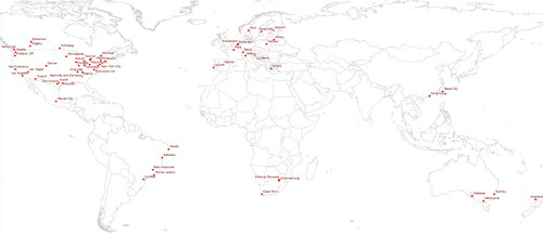
Table A1. Sampled cities.

City	Country	Population [persons]	Area [km²]	nGDP/capita [USD]	Household size [persons]
Adelaide	Australia	22,393	16	46,242.775	1.7
Albany	USA	98,111	55	59,633.028	2.2
Amsterdam	Netherlands	810,000	219	49,676.217	1.8
Athens	Greece	660,000	39	33,292.635	2.2
Atlanta	USA	472,522	345	47,024.482	2.3
Auckland	New Zealand	1,570,000	4,893	33,358.043	3.0
Austin	USA	947,890	772	46,605.293	2.5
Baltimore	USA	614,664	210	53,406.998	2.5
Basel	Switzerland	197,000	37	53,502.222	1.9
Belo Horizonte	Brazil	2,502,557	331	14,496.768	3.7
Boston	USA	673,184	125	64,869.603	2.4
Calgary	Canada	1,239,220	826	62,751.408	3.0
Cape Town	South Africa	3,840,000	2,461	10,882.016	3.4
Chicago	USA	2,704,958	590	52,351.825	2.6
Cleveland	USA	385,809	201	47,183.438	2.3
Columbus	USA	860,090	562	48,264.642	2.4
Curitiba	Brazil	1,750,000	434	18,273.472	3.0
Denver	USA	693,060	396	55,425.449	2.3
Detroit	USA	672,795	359	41,618.228	2.7
Edmonton	Canada	932,546	685	54,421.769	2.9
Hamilton	Canada	536,917	1,138	43,243.243	3.0
Helsinki	Finland	629,512	214	61,884.669	1.9
Hong Kong	China	7,310,000	1,104	32,550.000^†	2.8
Houston	USA	2,303,482	1,553	57,087.866	2.7
Indianapolis	USA	855,164	936	52,154.195	2.5
Johannesburg	South Africa	4,434,827	1,645	11,958.544	3.4
Knoxville	USA	186,239	255	44,285.714	2.1
Las Vegas	USA	632,912	352	44,556.962	2.8
Lisbon	Portugal	545,245	100	34,480.371	2.2
Ljubljana	Slovenia	279,756	164	36,911.577	2.3
Los Angeles	USA	3,976,322	1,214	56,905.132	2.8
Madrid	Spain	3,207,247	606	40,348.964	2.5
Manchester	UK	2,547,700	1,280	31,696.946	2.3
Melbourne	Australia	138,000	38	54,344.624	2.1
Mexico City	Mexico	8,874,724	1,485	12,680.817	3.4
Milano	Italy	1,350,000	182	44,777.986	1.8
Minneapolis	USA	413,651	140	54,948.391	2.3
Montreal	Canada	1,704,694	432	39,129.308	2.8
Nashville-Davidson	USA	660,388	1,231	45,710.708	2.4
New Orleans	USA	391,495	439	52,270.780	2.4
New York City	USA	8,537,673	784	62,367.239	2.7
Oslo	Norway	660,000	454	126,334.520	1.9
Paris	France	2,270,000	105	64,702.396	1.9
Philadelphia	USA	1,567,872	347	52,680.067	2.6
Pittsburgh	USA	303,625	143	49,277.825	2.1
Portland	USA	639,863	346	66,772.156	2.3
Pretoria Tshwane	South Africa	3,200,000	6,298	23,160.763	3.4
Recife	Brazil	1,555,039	218	9,753.454	3.2
Richmond	USA	223,170	155	53,882.726	2.3
Rio de Janeiro	Brazil	6,500,000	1,224	15,283.880	2.9
Rotterdam	Netherlands	620,000	208	43,570.960	1.9
Salvador	Brazil	2,920,000	693	13,710.129	3.1
San Antonio	USA	1,492,510	1,194	39,516.504	2.9
San Francisco	USA	870,887	121	65,156.394	2.3
Seattle	USA	704,352	217	61,177.153	2.1
Stockholm	Sweden	901,000	216	71,428.571	2.1
Sydney	Australia	205,000	26	58,545.613	2.1
Taipei City	Taiwan	2,704,974	272	23,549.287	2.6
Toronto	Canada	2,810,000	634	47,030.134	2.9
Tucson	USA	530,706	587	37,525.355	2.5
Vancouver	Canada	600,000	115	42,659.975	2.8
Vilnius	Lithuania	542,664	401	16,489.988	2.3
Warsaw	Poland	1,730,000	517	25,434.243	2.2
Winnipeg	Canada	705,244	464	42,440.318	2.9
Zaragoza	Spain	661,108	974	33,586.643	2.4

^† Retrieved from the World Bank.

Table A2. Ordinary least squares regression.

	Dependent: TrTime				Dependent: T1MeanCap
	Coef.	Std. coef.	p	VIF	Coef.	Std. coef.	p	VIF
PopDen	8.53E-05	0.035	0.365	1.704	−4.909E-04	−0.262	0.032	1.780
LBUAPer	9.560	0.067	0.265	1.968	−41.847	−0.355	0.010	2.044
HBUAPopDen	−0.001	−0.236	0.050	3.436	1.979E-04	0.078	0.348	3.651
GDPCap	−1.171E-04	−0.244	0.012	1.891	−3.09E-05	−0.085	0.320	3.077
DiePrice	6.978	0.250	0.006	1.593	−7.418	−0.304	0.040	2.697
Hsize	6.610	0.328	0.005	2.517	−9.481	−0.587	0.001	2.718
Cong	62.627	0.691	0.000	2.013	−37.472	−0.518	0.007	3.737
TrTime	–	–	–	–	0.214	0.268	0.088	3.560
HDD	–	–	–	–	−1.518E-04	−0.020	0.456	3.083
CDD	–	–	–	–	0.001	0.083	0.251	1.417
(Constant)	−6.860		0.272		61.845		0.000
	n = 64, F(7, 56) = 16.712 (p = 0.000), R² = 0.676, Adj. R² = 0.636, RMSE = 5.523, Durbin-Watson = 1.834				n = 54, F(10, 43) = 5.090 (p = 0.000), R² = 0.542, Adj. R² = 0.436, RMSE = 5.545, Durbin-Watson = 1.735

– : Not considered in the model.

Note: For variable names, see Table 1.

In regard to the predictors of travel time and CO₂ emissions, congestion level, GDP per capita, and household size were used to define the sample while for the following variables, all cities in the sample had values. If not, this study extracted the values from the original CDP database.

First, similar to the congestion level, an exposure variable in the travel model, the CO₂ model included, in addition to the land use, sociodemographic, and transportation characteristics of the city, the exposure variables of HDD (heating degree days) and CDD (cooling degree days) to consider climate-related energy consumption and CO₂ emissions. They are defined as the annual sum of the difference between Tr (reference temperature, 15.5 °C for HDD and 23 °C for CDD) and Td (daily temperature) no matter when Tr is higher (HDD) or lower (CDD) than Td: HDD = ΣMax(Tr − Td, 0) and CDD = ΣMax(Td − Tr, 0).

Besides, both travel distance and energy consumption rely on the fuel/energy price (Guzman et al., 2016), and was thus controlled for. Particularly, the dataset provided gasoline and diesel prices, but they had high collinearity. Therefore, this study selected the diesel price since it better accounts for variations in response variables.

As the most frequently analyzed land use variable, this study calculated population density with the data of population size and city area, provided by Nangini et al. (2019). They manually collected population and area data from Wikipedia, C40 (www.c40.org), and the U.S. Census Bureau. (Although data on population density were directly available from GEA, UITP, and World Bank, no types of data had more than half of the density values for the sample.)

In addition, this study evaluated city-level land use patterns using BUA (built-up area) variables as generated by Nangini et al. (2019) who also completed the QA of their data. Calculated from high-resolution Landsat-based satellite images, high BUA refers to contiguous cells with a population density of equal to or more than 1,500 persons/km² (and at least 50,000 people in the area) and low BUA to those with the density of equal to or more than 300 persons/km² (and at least 5,000 people in the total area) (Nangini et al., 2019). In particular, the proportion of low BUA was used as a simple sprawl index. Sprawl tends to be evaluated with a composite of multiple indicators. However, Laidley (2016) argued that such a multi-indicator index is difficult to apply to a large number of cities due to different data availability and further, the indicators are often misselected, which considerably distorts the index value. By comparison, although the sprawl index of this study—it follows Lopez and Hynes’s definition (Lopez & Hynes, 2003)—has the issue that the theoretical components of sprawl may not be reflected, the index is simple to calculate, its data are easy to collect—both of the index simplicity and data availability make the index highly applicable to various areas—and the values are insensitive to the area, boundary, and physical topography (Laidley, 2016). Thus, after comparing various indices, Laidley (2016) selected the low BUA proportion as a desirable sprawl measure as with this study.

While density is used as the opposite concept of sprawl, population density in the original dataset means gross density, which needs to be differentiated from net density (Forsyth et al., 2007; Gim, 2012). Thus, to supplement gross population density and the low BUA proportion as a sprawl index, this study considered high BUA population density. In total, nine exogenous (predicting) and two endogenous (mediating and outcome) variables were employed in this study (Table 1).

Table 1. Descriptive statistics.

Variables (units)	Descriptions	n	Mean	S.D.	Min	Max
Outcome
T1MeanCap (tCO2)	Per-capita CO2 emissions separated from all types of greenhouse gas emissions	55	9.614	7.332	0.602	30.849
Mediator/intermediary
TrTime (minutes)	Mean one-way travel time	65	30.788	9.176	13.333	75.000
Predictors
PopDen (persons/km²)	Population density	65	3,753.170	3,696.017	320.867	21,619.048
LBUAPer (%)	Proportion of the low-density built-up	65	0.314	0.066	0.164	0.487
HBUAPopDen (persons/km²)	Population density of the high-density built-up	65	3,590.847	2,790.835	1,018.154	13,071.756
GDPCap (USD/capita)	Nominal GDP per capita	64	44,667.084	19,031.972	9,753.454	126,334.520
DiePrice (USD/liter)	Fuel price for diesel	65	1.217	0.328	0.970	2.110
HSize (persons/household)	Mean household size	65	2.516	0.452	1.700	3.704
Cong (%)	Congestion level	65	0.275	0.101	0.100	0.660
HDD (°C)	Heating degree days	65	1,208.262	986.797	0	3,941.000
CDD (°C)	Cooling degree days	65	237.169	514.058	0	2,547.000

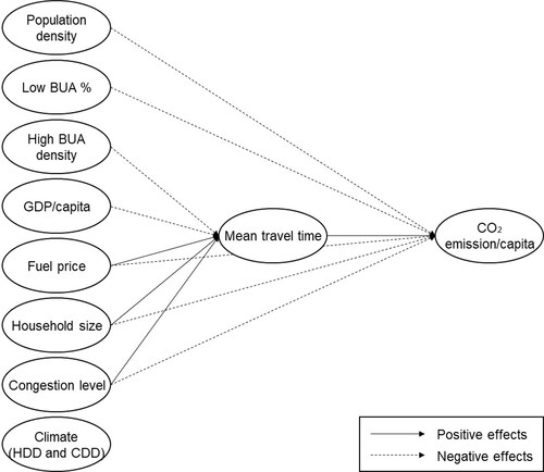
As shown in Figure 2, to evaluate the mediating effect of the travel time (Guzman & Orjuela, 2017), this study employed SEM. [It is computationally complex that the traditional regression-based approach specifies multiple independent variables to simultaneously estimate the mediating effects of the travel time. Thus, the approach analyzes independent variables one by one while controlling for the others as covariates.] Particularly, this study used exploratory PLS-SEM instead of confirmatory CB-SEM (covariance-based SEM) as conventionally used. In the same sense, this study tested indirect paths from all extraneous variables through the travel time mediator. A strength of PLS-SEM is that while CB-SEM requires a large sample size and a limited number of paths, PLS-SEM is free from these requirements. Thus, PLS-SEM can handle a complex model with a small sample as with the sample for this study.⁵ Furthermore, unlike the CB-SEM model for which a construct (latent variable) should ideally carry three to five indicators (observed variable) to be identifiable, the PLS-SEM model fully works with only one indicator per construct (or with a very large number of indicators) (Gim, 2019). In this study, all constructs have a single indicator except for the climate (F_Climate), which is formed (not reflected) by CDD and HDD (see Figure 3); PLS-SEM can specify formative constructs (arrows go from indicators to its construct) while CB-SEM has been developed mainly for the reflective measurement (arrows go from a construct to its indicators) (Gim, 2019).

Figure 2. Analytical model.

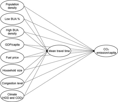
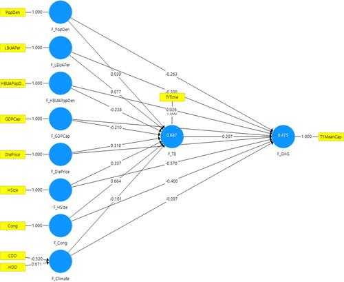
Figure 3. Structural equation model: standardized path coefficients and R².

Notes: For variable names, see Table 1. The figure was auto-generated by SmartPLS 3 and its fuller results are available online: https://drive.google.com/open?id=1LDADriaU5LJnkynrfTSpEw7JkBOM3i5R

4. Results

4.1. Correlation analysis

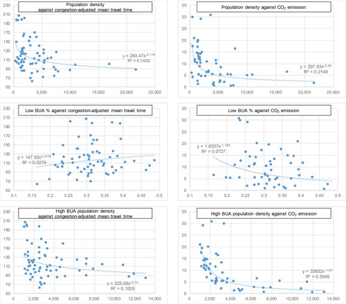
Before the main inferential statistics, this study checked the correlation between the three land use variables (i.e., gross population density, low BUA proportion, and high BUA population density) and the endogenous variables (Figure 4). Carbon emissions were separately provided from the total GHG emissions through methane correction and travel time was standardized by the TomTom congestion level.

Figure 4. Correlates of gross population density, low BUA proportion (sprawl), and high BUA population density (compactness).

Note: For power trend-lines and their R², see Figure A1.

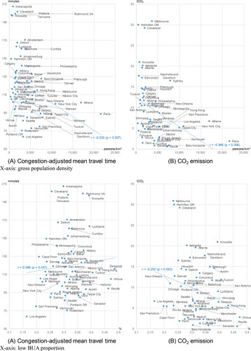
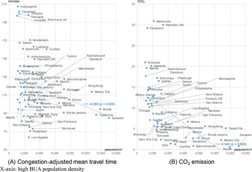
As shown in scatter plots, the gross and high BUA densities had inversely proportional relationships with the travel time and CO₂ emissions. Pearson’s correlation was modest to moderate (|r| = 0.29–0.55). In contrast, the correlation that the low BUA proportion as a sprawl measure had with each of the travel time and emissions was not significant or significant only at the 10% significance level. (Notably, the sprawl–CO₂ emission relationship was not positive, but negative; this will be discussed later.) [In fact, as expected, power trend-lines produced somewhat higher r² (0.03–0.59) than linear trend-lines (0.01–0.30), although no type of transformed variables (e.g., exponential, logarithmic, polynomial, and power) was found to be more significant than those in their original forms (see Figure A1). According to Gudipudi et al. (2016), a linear relationship was fitted in this study between population density and CO₂ emissions per capita.]

4.2. Structural equation modeling

In Figure 3 and Table 2, R² and SRMR show that the SEM model was well specified. Also, as PLS-SEM fit indices suggested by Dijkstra and Henseler (2015), the original values of d_ULS (squared Euclidean distance) and d_G (geodesic distance) are smaller than the upper bounds of their respective 95% and 99% confidence intervals, suggesting that the model has a good fit.

Table 2. Partial least squares structural equation modeling.

			Std. path coef.	p	Total effects	f²	R²	Adj. R²
F_PopDen	→	F_TB	0.039	0.306	0.039	0.003	0.687	0.642
F_LBUAPer	→		0.077	0.233	0.077	0.010
F_HBUAPopDen	→		−0.238	0.065	−0.238	0.050
F_GDPCap	→		−0.210	0.015	−0.210	0.075
F_DiePrice	→		0.310	0.011	0.310	0.143
F_HSize	→		0.337	0.008	0.337	0.147
F_Cong	→		0.664	0.000	0.664	0.658
F_Climate	→		−0.101	0.293	−0.101	0.018
F_PopDen	→	F_GHG	−0.263	0.006	−0.255	0.077	0.475	0.389
F_LBUAPer	→		−0.300	0.036	−0.284	0.085
F_HBUAPopDen	→		0.026	0.448	−0.024	0.000
F_GDPCap	→		−0.084	0.268	−0.128	0.007
F_DiePrice	→		−0.280	0.013	−0.216	0.061
F_HSize	→		−0.570	0.001	−0.500	0.220
F_Cong	→		−0.400	0.019	−0.262	0.086
F_Climate	→		−0.097	0.244	−0.118	0.010
F_TB	→		0.207	0.094	0.207	0.026
			Outer weights	p
CDD	→	F_Climate	−0.520	0.159
HDD	→		0.671	0.119
			n = 65, SRMR = 0.048 (cutoff < 0.10), d_ULS = 0.153 [cutoff < 1.089 (upper bound of the 95% confidence interval) and 1.345 (99%)], d_G = 0.082 [cutoff < 0.188 (95%) and 0.243 (99%)]

Note: For variable names, see Figure 3 and Table 1.

4.2.1. Direct effects on travel time

Table 2 firstly shows the direct effects of predicting variables on the mean travel time and carbon emissions. Relative to the emissions, a smaller number of variables (= 7) was used to account for more variation in the travel time. This implies that a variety of variables are involved in carbon emissions. Such a result is also relevant to the fact that the emissions are based widely on industry, waste, and electricity generation in addition to transportation.

In explaining variations in travel time, four non-land use control variables were all found to be significant; the 90% significant level was applied unless otherwise mentioned. As expected, the congestion level as an exposure variable became the most critical in increasing the travel time (standard coefficient = 0.691). As the second most important variable, household size extended travel (0.328), which is consistent with the findings of most individual-level studies (Cao et al., 2007a; Gim, 2011).

Meanwhile, the economic level (GDPCap) turned out to reduce travel time. This differs from the consistent argument of those studies conducted at the individual level that individual/household income is among the most critical variables in increasing travel (Cao et al., 2007b; Zegras, 2004). However, since the unit of analysis of this study is not the individual, but the city, the finding may indicate that wealthy/competitive cities are usually equipped with advanced and efficient transportation infrastructure, which shortens/saves the travel time in general.

Higher fuel prices (DiePrice) also led to longer travel time, which is again inconsistent with the findings of individual-level studies in that they usually reported a negative relationship (Ewing et al., 2018). However, in this city-level study, the positive relationship may suggest that in international comparisons, wealthier and more advanced cities with higher costs of living, including fuel price, allow people to travel further.

As a second explanation, the positive relationship partially supports Khazzoom’s rebound effect (Khazzoom, 1980; Saunders, 1992). That is, (vehicle-technology development reduces the energy consumption and driving costs, but in the long run) lesser operational costs directly cause further and more travel by automobile and fuel bill savings indirectly facilitate distant trips. Particularly regarding land use, the fuel cost savings–distant travel relationship is concerned with the compensatory hypothesis that residents in compact cities reduce daily regular travel, but as a compensation for limited urban travel, they increase distant travel using the cost savings on weekends/holidays (Gim, 2017; Holden & Norland, 2005). Fertner and Große’s review (Fertner & Große, 2016) emphasized that compact cities as innovation centers increase energy efficiency, but the rebound effect may generate tradeoffs and thus necessitate accompanying measures such as efficient public transportation systems.

A third possibility is that the higher fuel price–more travel time relationship implies a modal shift. Creutzig (2014) assumed a simplified economic model for a city with one center and two travel modes: automobile and public transit. The study reported that if fuel prices rise, the mode shares of the automobile and transit are lowered and heightened, respectively, and subsequently, CO₂ emissions are reduced. Meanwhile, transit is slower (Gim, 2018), so the modal share change by higher fuel prices is in line with the positive fuel price–travel time relationship. [In the later part of this study, higher fuel prices are found to reduce CO₂ emissions, which also echoes Creutzig’s analytical results (2014).]

Among the three land use variables—gross population density, low BUA proportion, and high BUA population density—only the high BUA density, which represents compactness, significantly reduced travel. This result supports Hunter and Haughton’s definition of compact cities as those with dense urban cores/nuclei, but not with generally high density (Hunter & Haughton, 2003) and Brotchie’s argument that compact developments increase not the overall density, but the density in a particular area (Brotchie, 1992). These studies are concerned with the concept of transit-oriented development (TOD), which aims to reduce travel by specifying such a dense area as public transportation nodes or trip destination clusters that are equipped with work, shopping, and recreational facilities (Burton, 2002). Similar to this study, Ewing et al. (2018) reported that in contrast to Newman and Kenworthy’s theory of the negative gross density–individual automobile use relationship, VMT is strongly associated with the compactness/sprawl index rather than the density itself. The high BUA density as a land use representative had a smaller effect (standardized coefficient) than socioeconomic control variables. This is in line with the consistent findings of the literature (Gim, 2018).

4.2.2. Direct effects on CO₂ emissions

In accounting for CO₂ emissions, six out of ten variables (= seven used for explaining travel time + travel time + HDD and CDD for reflecting climate conditions) were significant (see Figure 5). Particularly, travel time increased carbon emissions. In the Baltimore metropolitan area, Liu and Shen (2011) similarly found a positive relationship between VMT and energy use (a proxy for carbon emissions). According to the significant travel time–emission path, the travel time was suspected to have mediating effects on the relationships between other independent variables and CO₂ emissions (this suspicion is tested below). In this sense, this study is similar to Liu and Shen’s metropolitan-scale analysis (2011). However, there are differences. They considered only the indirect path of density–VMT–energy use, not the direct density–energy use path. Also, their SEM model specified only population density without consideration of other land use aspects.

Figure 5. Analytical results.

Among the four control variables in predicting travel time variations (i.e., per-capita GDP, fuel price, household size, and congestion level), all of which were significant, per-capita GDP was insignificant unlike the others in explaining CO₂ emissions. (However, this variable can still affect the emissions indirectly through the GDP–travel time–CO₂ emission path.) This result is inconsistent with the conclusion of a growing body of research that economic growth necessitates more emissions (Saboori et al., 2014). Moreover, the result rejects/details the argument of Ou et al. (2017). In their regression analysis, the GDP of the city was negatively associated with CO₂ emissions. However, CO₂ emissions were not observed, but estimated using daily travel data from travel surveys. Thus, they actually confirmed the negative GDP–travel relationship, which was supported in this study. [Meanwhile, relative to this study on a global scale, Rahman’s review (2017) showed that regionally limited individual studies tended to report contradictory (i.e., significant, insignificant, and partially significant) results on the income/economic growth–CO₂ relationship.]

Among the three significant control variables, fuel price had a negative relationship with CO₂ emissions. That is, residents in cities with high fuel prices spend less energy, so the prices may “directly” reduce CO₂ generation. This finding supports Creutzig’s theoretical/mathematical results (2014) based on a simple economic model, that is, it suggests “indirect” effects on CO₂ reductions through those on transportation [higher prices → use of public transit in place of the automobile (modal shift) → less CO₂ emissions]. Notably, as discussed above, fuel prices may indicate the economic power/competitiveness of a city (accordingly, the positive fuel price–travel time relationship occurs) as well as how it implements tax policies for energy saving and emission reduction (Li & Yao, 2020). Thus, the less energy use/CO₂ emissions might be attributed not only to energy saving behavior by residents, but also to energy efficiency/carbon reduction technologies of such an advanced city. In a similar context, Bettencourt et al. (2007) found that cities in developed regions emit less on a per capita basis owing to infrastructure efficiency. Also, according to Gudipudi et al. (2016), why cities in developing regions present larger per-capita emissions is related partially to the type and deficiency of the basic infrastructure.

As the second control variable, while the household size was likely to increase mean travel time as stated before, it had a negative relationship with per-capita CO₂ emissions. This is consistent with a priori knowledge that in comparison to multi-person households, single-person households generate more per-capita waste due to inefficient material and energy use. Similarly, empirical studies (Jiang & Hardee, 2011; Zhu & Peng, 2012) found that smaller household sizes tend to raise residential consumption, leading to higher carbon emissions. Indeed, the variable was found to be the strongest and second strongest determinant of CO₂ emissions and travel time, respectively.

The third control variable, congestion level, exerted a strong effect on CO₂ emissions as well as on travel time. According to the standardized coefficient, it had the strongest and second strongest influence on each of the travel time and emissions. [In Table 2, f² also shows that on travel time, congestion and household size are the first and second influences in magnitude and the second and first on CO₂ emissions, respectively.] Meanwhile, the congestion effect on the emissions was negative (as opposed to the positive effect on travel time). This may be because congestion reduces speed, which increases fuel efficiency to a degree. In a similar vein, Barth and Boriboonsomsin (2008) conceptualized the effect of speed management that if speed is controlled from free-flow conditions, CO₂ is less generated. Another possibility is that under the same travel time (ceteris paribus) condition (it is because travel time is controlled for), speed reductions by congestion denote shorter trip lengths (i.e., choice of closer alternative destinations owing to the traffic calming effect) and subsequently, lower CO₂ emissions.

Among the three land use variables, gross population density and low BUA proportion were directly and negatively related to CO₂ emissions. The result on gross population density is in line with the consistent argument of previous studies (Makido et al., 2012; Rybski et al., 2017) and may be due to the economies of scale/agglomeration through the efficient use of the energy infrastructure. [Meanwhile, high BUA population density may still indirectly affect CO₂ emissions since it has a relationship with travel time, which in turn has a relationship with CO₂ emissions (to be discussed later).] Secondly, unlike our initial expectation, the low BUA proportion as a sprawl index also led to low CO₂ emissions. This paradox is further analyzed through SEM.

In summary, regarding their direct effects, urban center density reduces travel time and overall density reduces carbon emissions. Likewise, based on 7-year longitudinal data of 60 U.S. Metropolitan Statistical Areas, Kashem et al. (2014) argued that cities with notable centers (i.e., high density of their high BUA) encourage people to drive less and at the same time, cities with high overall density tend to have low levels of ambient ozone and fine particulate matter.

While the significance of the travel time–CO₂ emission relationship was confirmed, three variables (i.e., fuel price, household size, and congestion level) had the opposite effects on the travel time and emissions. Thus, in the next section, this study checks the mediation by travel time and how its positive indirect and negative direct effects on CO₂ emissions are traded off at the final total effect level. We estimate partial least squares one-sided SEM by resampling 10,000 times with the actual sample size.

4.2.3. Mediating effect of travel time

Regarding the mediation by travel time, Table 2 shows that the path of F_TB → F_GHG is significant. Thus, several predictors are considered to affect CO₂ emissions through the travel time mediator. First, among the four variables controlled for in predicting travel time—GDP per capita, fuel price, household size, and congestion level—GDP only indirectly affected the emissions through the GDP–travel time–emission path (i.e., the GDP–emission relationship was completely mediated by travel time). The other three variables had both direct and indirect effects (i.e., incomplete mediation). Their direct effects were all positive on travel time, but negative on CO₂ emissions. As the most important result of SEM, in terms of the total effect, the negative effect overwhelmed the positive effect. Thus, the variables ultimately brought about less CO₂ generation.

Among the land use variables, high BUA population density only indirectly affected per-capita CO₂ emissions by reducing travel (i.e., complete mediation). By comparison, the other two land use variables (i.e., gross population density and low BUA proportion as a sprawl index) were only directly involved in emission reduction. As expected, compact developments with high BUA density and outstanding urban cores/nuclei reduced travel and subsequently tailpipe CO₂ emissions. In contrast, although the overall density in the entire city was not meaningful in travel variations, which reaffirms the consistent findings of the literature (Ewing & Cervero, 2010; Handy, 2005), it directly reduced per-capita CO₂ emissions in those sectors unrelated to transportation. In relation to the economies of scale/agglomeration, urban infrastructure is better shared in dense cities, which may subsequently reduce the per-capita emissions.

If the study area is expanded from the frequently studied U.S. and Europe to elsewhere, the sprawl index (low BUA proportion) had an insignificant—albeit positive (coefficient = 0.077)—effect on travel. However, it directly reduced CO₂ emissions. Seemingly, this contradicts the findings of the existing literature. Actually, the city-level model controlled for density variables. Thus, under the same overall density (ceteris paribus) condition, a larger proportion of low BUA indicates more population living in the remaining smaller high BUA; indeed, in the dataset, low BUA proportion was calculated based not on the entire city area, but on the sum of the low and high BUAs. Thus, this result might be attributed to energy use efficiency by the economies of agglomeration. From the perspective of the paradox of intensification (Melia et al., 2011), another plausible explanation is that by transferring the development pressure, sprawl aggravates the environment of hinterland areas, but protects that of the studied core city, including green spaces. [In fact, the inverse relationship between density and the area of green spaces has been reported. Based on 11-year panel data for cities in China, Wang and Yuan (2017) found that density reduces per-capita urban greenness.]

5. Summary

This study aimed to be an analysis at a global scale of how between-city variations in land use including population density affect both travel time and CO₂ emissions. Specifically, based on data compiled and edited by Nangini et al. (2019), this study differed in that the land use–travel time–carbon emission relationship was analyzed on a global scale, beyond a national/regional scale with one/several countries, using city-level emission data that were individually reported, not estimated from travel survey data or satellite images. To evaluate the mediation of travel time according to the above conceptual relationship, this study specified an SEM model. As research variables, land use characteristics were centered on population density: gross population density, proportion of the low-density built-up area (sprawl measure), and population density of the high-density built-up area (compactness measure). City-level economic, social, transportation, energy, and climate conditions were controlled for.

Empirical results about direct effects can be summarized as follows.

• Among the control variables, congestion and household size were the most important in increasing travel time.

• As a measure of the economic status, per-capita GDP shortened travel time, which contradicts the findings of individual-level studies (Cao et al., 2007b; Zegras, 2004). However, considering that the unit of analysis was the city, this may be because the competitive transportation infrastructure of such an affluent city facilitated efficient travel.

• Unlike the argument of the literature (Ewing et al., 2018), fuel price extended travel time. This may imply the rebound effect (where fuel cost savings ultimately cause further travel) or the modal shift (through the path of fuel price increases–shift to (slower) public transit–travel time increases).

• Out of the above four controls, household size, congestion level, and fuel price significantly reduced CO₂ emissions in descending order of their magnitudes. Notably, in comparison to their positive effects on travel time, the effects were negative on the emissions.

• Regarding household size, the result confirmed the expectation that smaller households are less efficient in consuming resources/energy.

• The congestion effect on emission reductions may be caused by (1) the speed management effect, which accordingly raises fuel efficiency (Barth & Boriboonsomsin, 2008), or (because speed reductions under the controlled/same travel time condition denote trip length reductions) (2) the traffic calming effect and subsequent choice of closer alternative destinations.

• Higher fuel prices can reduce the emissions by directly encouraging energy savings as well as indirectly facilitating the modal shift to public transportation (Creutzig, 2014). Assuming that fuel prices reflect the costs of living/economic conditions and competitiveness of a city, the result may also be explained by its effective tax policy and advanced energy-efficient technology/infrastructure.

• The effects of the fuel price (USD/liter) were negative on travel time (minutes) and positive on carbon emissions (tCO₂). In the sample, the price was the highest in Oslo, Norway (2.11) in which the mean time and emissions were 26.0 and 1.469, respectively. The fuel was among the cheapest in Atlanta, Georgia, U.S. (0.97) and Winnipeg, Canada (1.16) where the mean time was shorter (25.5 and 23.3) and the emissions were larger (19.588 and 5.633) in line with the findings of this study. As with the fuel price, the household size had differing effects on the travel time and emissions. The size was the largest in Belo Horizonte, Brazil (3.7), Mexico City, Mexico (3.4), and Johannesburg, South Africa (3.4), each of which had the travel time and emissions of 34.4, 75.0, and 45.7 minutes and 0.849, 2.312, and 4.821 tons. In the three above-mentioned cities (Oslo, Atlanta, and Winnipeg), the household size was smaller (1.9, 2.3, and 2.9 persons) and accordingly presented shorter travel time (26.0, 25.5, 23.3 minutes) and more carbon emissions (1.469, 19.588, and 5.633), which also confirms the empirical findings of this study. Notably, ceteris paribus, one-unit increases in the fuel price and household size would result in the travel time increase of 6.978 and 6.610 minutes and the emission reduction of 7.418 and 9.481 tons (see Table A2).

The SEM model also confirmed mediation by travel time. Specifically, per-capita GDP was mediated completely (i.e., it only had an indirect effect on CO₂ emissions) and fuel price, household size, and congestion level incompletely (i.e., they had both direct and indirect effects). The positive indirect effects of these three variables were entirely canceled out by their negative direct effects. Overall, they reduced CO₂ emissions.

Regarding land use, compact developments with high density in urban cores/nuclei (high-density built-up) reduced travel and subsequently, CO₂ emissions, partially because the nuclei work as public transit nodes/trip destination clusters, that is, TOD is facilitated) (complete mediation). In contrast, while the overall density of a city had no effects on travel, reaffirming the argument of the transportation literature (Ewing & Cervero, 2010; Handy, 2005), it directly reduced transportation-unrelated per-capita emissions possibly because the economies of scale generate the sharing/efficient use of the energy infrastructure, supporting the findings of the environmental policy literature (Makido et al., 2012). (That is, as for the direct effects, travel hinged on urban core density and the emissions on overall density). Furthermore, the proportion of the low-density built-up directly reduced the emissions. One might interpret that this implies the paradox of intensification (Melia et al., 2011) that sprawl can protect the environment of a city at the cost of that of suburban/rural areas. However, such an interpretation should be taken with great caution. Sprawl occurs with or without strong urban cores and at the fringes of existing urban areas or far from them (e.g., leapfrog development). Furthermore, studies (De Ridder et al., 2008; Fan & Song, 2009) have found that sprawl imposes an environmental or health burden on the central city.

A notable limitation of the study is that among 343 cities that were initially considered (or 187 cities in the CDP dataset), empirical analyses only used 65 according to their data availability. Furthermore, the final sample better represented European and U.S. cities than those in other continents. As with McIntosh et al. (2014), these must have affected the geographical transferability of the findings of this study. Thus, further research is desirable to see if the findings are applicable to cities at different ranges of exogenous and endogenous variables. Also, attitudinal variables have consistently been reported as major travel determinants (Ewing & Cervero, 2010), but this study did not consider them. Therefore, for more accurate estimation, future studies are recommended to control for these possible confounders. Lastly, particularly concerning the land use–travel relationship, the reverse or even reciprocal causality has been suspected (Gim, 2013; Handy, 2005; Holz-Rau & Scheiner, 2019) but not tested in this study, so the suspicion should be critically examined in the future, desirably with longitudinal data.

Acknowledgements

This work was supported by ‘Overseas Training Expenses for Humanities & Social Sciences’ through Seoul National University (SNU).

Disclosure statement

No potential conflict of interest was reported by the authors.

Notes

1 Alternately, the discrepancy of analytical results between aggregate and disaggregate studies may be attributed to aggregation bias (i.e., ecological fallacy) according to which aggregate studies have been greatly reduced since the mid-1990s (Ewing et al., 2018; Handy, 2005). Another possibility given by Ewing et al. (2018) is omitted variable bias (i.e., spatial multicollinearity), that is, the discrepancy is because the observed density effect encompasses the effects of other land use variables (e.g., parking availability and destination accessibility) (Forsyth et al., 2007). On the one hand, spatial multicollinearity is interpreted to argue that the actual effect of a separate land use variable is rather modest if others are controlled for (Bagley & Mokhtarian, 2002). On the other hand, it is used to justify land use interventions (Schimek, 1996; Zhang, 2004), in the sense that despite the modest effect of one variable, its composite effect magnified through the multicollinearity could be meaningful (Gim, 2013).

2 According to Goodhue et al. (2012), this study conducted regression analyses on travel time and carbon emissions before structural equation modeling (SEM) as its main analytical technique. Results from the regression models were consistent with those of the SEM model in every sense including the significance and relative magnitude of each path (see Table A2).

3 In addition to the original variable of income/GDP/economic growth, its squared form has frequently been analyzed to check the significance of the environmental Kuznets curve. In a preliminary analysis, however, squared GDP per capita was insignificant and subsequently excluded from the final model. Rahman’s review (2017) also suggested that the curve is not or only partially present.

4 Alternative data were available, such as GDP/capita by CDP and GDP-PPP/capita (GDP/capita at purchasing power parity) by each of the authors (Nangini et al. 2019), GEA (Gesellschaft für Entstaubungsanlagen), UITP (Union Internationale des Transports Publics), and World Bank. They all had more missing cases than the data employed in this study.

5 Land use variables may affect the congestion level. However, SEM specified it to be extraneous. A preliminary analysis showed that the correlation between these variables and congestion level is insignificant. Likewise, the VIF of the congestion in the travel time regression model was just 2.013 (see Table A2). Karathodorou et al. (2010) similarly found that while urban density influences fuel consumption (accordingly, CO₂ emissions), it particularly affects travel distances (and the automobile stock of the city) rather than unit-distance energy consumption (i.e., congestion). Liu and Shen (2011) also found that the effect of compact urban form on the reduction of travel speed is merely modest.

Appendices

Figure A1. Scatter plots and power trend-lines of land use variables against travel time and CO₂ emissions.

Note: For comparison, see Figure 3.

References

- Bagley, M. N., & Mokhtarian, P. L. (2002). The impact of residential neighborhood type on travel behavior: A structural equations modeling approach. The Annals of Regional Science, 36(2), 279–297. https://doi.org/https://doi.org/10.1007/s001680200083
- Barth, M., & Boriboonsomsin, K. (2008). Real-world carbon dioxide impacts of traffic congestion. Transportation Research Record: Journal of the Transportation Research Board, 2058(1), 163–171. https://doi.org/https://doi.org/10.3141/2058-20
- Bechle, M. J., Millet, D. B., & Marshall, J. D. (2011). Effects of income and urban form on urban NO2: Global evidence from satellites. Environmental Science & Technology, 45(11), 4914–4919. https://doi.org/https://doi.org/10.1021/es103866b
- Bettencourt, L. M. A., Lobo, J., Helbing, D., Kühnert, C., & West, G. B. (2007). Growth, innovation, scaling, and the pace of life in cities. PNAS, 104(17), 7301–7306.
- Boarnet, M., & Crane, R. (2001). The influence of land use on travel behavior: Specification and estimation strategies. Transportation Research Part A, 35(9), 823–845.
- Brotchie, J. (1992). The changing structure for cities. Urban Futures, S5, 13–23.
- Buchanan, N., Barnett, R., Kingham, S., & Johnston, D. (2006). The effect of urban growth on commuting patterns in Christchurch, New Zealand. Journal of Transport Geography, 14(5), 342–354. https://doi.org/https://doi.org/10.1016/j.jtrangeo.2005.10.008
- Burton, E. (2002). Measuring urban compactness in UK towns and cities. Environment and Planning B: Planning and Design, 29(2), 219–250. https://doi.org/https://doi.org/10.1068/b2713
- Cao, X., & Fan, Y. (2012). Exploring the influences of density on travel behavior using propensity score matching. Environment and Planning B: Planning and Design, 39(3), 459–470. https://doi.org/https://doi.org/10.1068/b36168
- Cao, X., Mokhtarian, P. L., & Handy, S. L. (2007a). Cross-sectional and quasi-panel explorations of the connection between the built environment and auto-ownership. Environment and Planning A: Economy and Space, 39(4), 830–847. https://doi.org/https://doi.org/10.1068/a37437
- Cao, X., Mokhtarian, P. L., & Handy, S. L. (2007b). Do changes in neighborhood characteristics lead to changes in travel behavior? A structural equations modeling approach. Transportation, 34(5), 535–556. https://doi.org/https://doi.org/10.1007/s11116-007-9132-x
- Choi, H., Nakagawa, D., Matsunaka, R., & Oba, T. (2012). International research on the relationship between urban structure and transportation energy consumption according to economic level. Australasian Journal of Regional Studies, 18(1), 128–149.
- Cooper, H. M., & Hedges, L. V. (1994). The handbook of research synthesis. Russell Sage Foundation.
- Creutzig, F. (2014). How fuel prices determine public transport infrastructure, modal shares and urban form. Urban Climate, 10, 63–76. https://doi.org/https://doi.org/10.1016/j.uclim.2014.09.003
- De Ridder, K., Lefebre, F., Adriaensen, S., Arnold, U., Beckroege, W., Bronner, C., Damsgaard, O., Dostal, I., Dufek, J., Hirsch, J., IntPanis, L., Kotek, Z., Ramadier, T., Thierry, A., Vermoote, S., Wania, A., & Weber, C. (2008). Simulating the impact of urban sprawl on air quality and population exposure in the German Ruhr area. Part II: Development and evaluation of an urban growth scenario. Atmospheric Environment, 42(30), 7070–7077. https://doi.org/https://doi.org/10.1016/j.atmosenv.2008.06.044
- Dijkstra, T. K., & Henseler, J. (2015). Consistent partial least squares path modeling. MIS Quarterly, 39(2), 297–316. https://doi.org/https://doi.org/10.25300/MISQ/2015/39.2.02
- Dujardin, S., Pirart, F., Brevers, F., Marique, A. F., & Teller, J. (2012). Home-to-work commuting, urban form and potential energy savings: A local scale approach to regional statistics. Transportation Research Part A, 46(7), 1054–1065.
- Ewing, R., & Cervero, R. (2001). Travel and the built environment: A synthesis. Transportation Research Record: Journal of the Transportation Research Board, 1780(1), 87–113. https://doi.org/https://doi.org/10.3141/1780-10
- Ewing, R., & Cervero, R. (2010). Travel and the built environment: A meta-analysis. Journal of the American Planning Association, 76(3), 265–294. https://doi.org/https://doi.org/10.1080/01944361003766766
- Ewing, R., Bartholomew, K., Winkelman, S., Walters, J., & Chen, D. (2008). Growing cooler: The evidence on urban development and climate change. Urban Land Institute.
- Ewing, R., Hamidi, S., Tian, G., Proffitt, D., Tonin, S., & Fregolent, L. (2018). Testing Newman and Kenworthy’s theory of density and automobile dependence. Journal of Planning Education and Research, 38(2), 167–182. https://doi.org/https://doi.org/10.1177/0739456X16688767
- Fan, Y., & Song, Y. (2009). Is sprawl associated with a widening urban-suburban mortality gap? Journal of Urban Health: Bulletin of the New York Academy of Medicine, 86(5), 708–728. https://doi.org/https://doi.org/10.1007/s11524-009-9382-3
- Fertner, C., & Große, J. (2016). Compact and resource efficient cities? Synergies and trade-offs in European cities. European Spatial Research and Policy, 23(1), 65–79. https://doi.org/https://doi.org/10.1515/esrp-2016-0004
- Filion, P., McSpurren, K., & Appleby, B. (2006). Wasted density? The impact of Toronto’s residential-density-distribution policies on public-transit use and walking. Environment and Planning A: Economy and Space, 38(7), 1367–1392. https://doi.org/https://doi.org/10.1068/a37414
- Fontaras, G., Zacharof, N.-G., & Ciuffo, B. (2017). Fuel consumption and CO2 emissions from passenger cars in Europe – Laboratory versus real-world emissions. Progress in Energy and Combustion Science, 60, 97–131. https://doi.org/https://doi.org/10.1016/j.pecs.2016.12.004
- Forsyth, A., Oakes, J. M., Schmitz, K. H., & Hearst, M. (2007). Does residential density increase walking and other physical activity? Urban Studies, 44(4), 679–697. https://doi.org/https://doi.org/10.1080/00420980601184729
- Gim, T.-H T. (2013). The relationships between land use measures and travel behavior: A meta-analytic approach. Transportation Planning and Technology, 36(5), 413–434. https://doi.org/https://doi.org/10.1080/03081060.2013.818272
- Gim, T.-H. T. (2011). A comparison of the effects of objective and perceived land use on travel behavior. Growth and Change, 42(4), 571–600. https://doi.org/https://doi.org/10.1111/j.1468-2257.2011.00568.x
- Gim, T.-H. T. (2012). A meta-analysis of the relationship between density and travel behavior. Transportation, 39(3), 491–519. https://doi.org/https://doi.org/10.1007/s11116-011-9373-6
- Gim, T.-H. T. (2017). Investigating travel utility elements in association with travel time and mode choice: the case of Seoul. Transportation Planning and Technology, 40(6), 641–660. https://doi.org/https://doi.org/10.1080/03081060.2017.1325136
- Gim, T.-H. T. (2018). Land use, travel utility, and travel behavior: An analysis from the perspective of the positive utility of travel. Papers in Regional Science, 97(S1), S169–S192. https://doi.org/https://doi.org/10.1111/pirs.12239
- Gim, T.-H. T. (2019). Examining the effects of residential self-selection on internal and external validity: an interaction moderation analysis using structural equation modeling. Transportation Letters, 11(5), 275–286. https://doi.org/https://doi.org/10.1080/19427867.2017.1338544
- Giuliano, G., & Dargay, J. (2006). Car ownership, travel and land use: A comparison of the US and Great Britain. Transportation Research Part A, 40, 106–124.
- Goodhue, D. L., Lewis, W., & Thompson, R. (2012). Comparing PLS to Regression and LISREL: A Response to Marcoulides, Chin, and Saunders. MIS Quarterly, 36(3), 703–716.
- Gudipudi, R., Fluschnik, T., Ros, A. G. C., Walther, C., & Kropp, J. P. (2016). City density and CO2 efficiency. Energy Policy, 91, 352–361. https://doi.org/https://doi.org/10.1016/j.enpol.2016.01.015
- Guzman, L. A., & Orjuela, J. P. (2017). Linking a transport dynamic model with an emissions model to aid air pollution evaluations of transport policies in Latin America. Transportmetrica B: Transport Dynamics, 5(3), 265–280.
- Guzman, L. A., de la Hoz, D., & Monzón, A. (2016). Optimization of transport measures to reduce GHG and pollutant emissions through a LUTI modeling approach. International Journal of Sustainable Transportation, 10(7), 590–603. https://doi.org/https://doi.org/10.1080/15568318.2015.1033039
- Handy, S. (2005). Does the built environment influence physical activtiy? Examining the evidence: Critical assessment of the literature on the relationships among transportation, land use, and physical activity. T. R. Board
- Holden, E., & Norland, I. T. (2005). Three challenges for the compact city as a sustainable urban form: Household consumption of energy and transport in eight residential areas in the Greater Oslo Region. Urban Studies, 42(12), 2145–2166. https://doi.org/https://doi.org/10.1080/00420980500332064
- Holz-Rau, C., & Scheiner, J. (2019). Land-use and transport planning – A field of complex cause-impact relationships. Thoughts on transport growth, greenhouse gas emissions and the built environment. Transport Policy, 74, 127–137. https://doi.org/https://doi.org/10.1016/j.tranpol.2018.12.004
- Hunter, C., & Haughton, G. (2003). Sustainable cities. Routledge.
- Jiang, L., & Hardee, K. (2011). How do recent population trends matter to climate change? Population Research and Policy Review, 30(2), 287–312. https://doi.org/https://doi.org/10.1007/s11113-010-9189-7
- Karathodorou, N., Graham, D. J., & Noland, R. B. (2010). Estimating the effect of urban density on fuel demand. Energy Economics, 32(1), 86–92. https://doi.org/https://doi.org/10.1016/j.eneco.2009.05.005
- Kashem, S. B., Irawan, A., & Wilson, B. (2014). Evaluating the dynamic impacts of urban form on transportation and environmental outcomes in US cities. International Journal of Environmental Science and Technology, 11(8), 2233–2244. https://doi.org/https://doi.org/10.1007/s13762-014-0630-z
- Kenworthy, J. R., & Laube, F. B. (1999). Patterns of automobile dependence in cities: An international overview of key physical and economic dimensions with some implications for urban policy. Transportation Research Part A, 33(7), 691–723.
- Khazzoom, D. J. (1980). Economic implications for mandated efficiency in standards for household appliances. Energy Journal, 1(4), 21–40.
- Laidley, T. (2016). Measuring sprawl: A new index, recent trends, and future research. Urban Affairs Review, 52(1), 66–97. https://doi.org/https://doi.org/10.1177/1078087414568812
- Levinson, H., & Wynn, F. H. (1963). Effects of density on urban transportation requirements. Highway Research Record, 2, 38–64.
- Li, X., & Yao, X. (2020). Can energy supply-side and demand-side policies for energy saving and emission reduction be synergistic?–- A simulated study on China's coal capacity cut and carbon tax. Energy Policy, 138, 111232. https://doi.org/https://doi.org/10.1016/j.enpol.2019.111232
- Light, R. J., & Pillemer, D. B. (1984). Summing up: The science of reviewing research. Harvard University Press.
- Liu, C., & Shen, Q. (2011). An empirical analysis of the influence of urban form on household travel and energy consumption. Computers, Environment and Urban Systems, 35(5), 347–357. https://doi.org/https://doi.org/10.1016/j.compenvurbsys.2011.05.006
- Lopez, R., & Hynes, H. P. (2003). Sprawl in the 1990S measurement, distribution, and trends. Urban Affairs Review (Thousand Oaks, Calif.), 38(3), 325–355. https://doi.org/https://doi.org/10.1177/1078087402238805
- Makido, Y., Dhakal, S., & Yamagata, Y. (2012). Relationship between urban form and CO2 emissions: Evidence from fifty Japanese cities. Urban Climate, 2, 55–67. https://doi.org/https://doi.org/10.1016/j.uclim.2012.10.006
- McIntosh, J., Trubka, R., Kenworthy, J., & Newman, P. (2014). The role of urban form and transit in city car dependence: Analysis of 26 global cities from 1960 to 2000. Transportation Research Part D: Transport and Environment, 33, 95–110. https://doi.org/https://doi.org/10.1016/j.trd.2014.08.013
- Melia, S., Parkhurst, G., & Barton, H. (2011). The paradox of intensification. Transport Policy, 18(1), 46–52. https://doi.org/https://doi.org/10.1016/j.tranpol.2010.05.007
- Mindali, O., Raveh, A., & Salomon, I. (2004). Urban density and energy consumption: A new look at old statistics. Transportation Research Part A, 38, 143–162.
- Mitchell, R. B., & Rapkin, C. (1954). Urban traffic: A function of land use. Columbia University Press.
- Naess, P. (2012). Urban form and travel behavior: Experience from a Nordic context. Journal of Transport and Land Use, 5(2), 21–45. https://doi.org/https://doi.org/10.5198/jtlu.v5i2.314
- Nangini, C., Peregon, A., Ciais, P., Weddige, U., Vogel, F., Wang, J., Bréon, F.-M., Bachra, S., Wang, Y., Gurney, K., Yamagata, Y., Appleby, K., Telahoun, S., Canadell, J. G., Grübler, A., Dhakal, S., & Creutzig, F. (2019). A global dataset of CO2 emissions and ancillary data related to emissions for 343 cities. Scientific Data, 6, 180280. https://doi.org/https://doi.org/10.1038/sdata.2018.280
- Newman, P., & Kenworthy, J. (2006). Urban design to reduce automobile dependence. Opolis, 2(1), 35–52.
- Newman, P., & Kenworthy, J. (2011). Peak car use: Understanding the demise of automobile dependence. World Transport Policy and Practice, 17(2), 31–42.
- Newman, P., & Kenworthy, J. (2015). The end of automobile dependence: How cities are moving beyond car-based planning. Island Press.
- Newman, P., & Kenworthy, J. R. (1989a). Cities and automobile dependence: An international sourcebook. Gower Technical.
- Newman, P., & Kenworthy, J. R. (1989b). Gasoline consumption and cities: A comparison of US cities with a global survey. Journal of the American Planning Association, 55(1), 24–37. https://doi.org/https://doi.org/10.1080/01944368908975398
- Ou, Y., Nakagawa, D., Matsunaka, R., & Oba, T. (2017). The analysis of CO2 emission by private cars in Chinese cities and international comparison. Urban and Regional Planning Review, 4, 185–201. https://doi.org/https://doi.org/10.14398/urpr.4.185
- Rahman, M. M. (2017). Do population density, economic growth, energy use and exports adversely affect environmental quality in Asian populous countries? Renewable and Sustainable Energy Reviews, 77, 506–514. https://doi.org/https://doi.org/10.1016/j.rser.2017.04.041
- Rajamani, J., Bhat, C. R., Handy, S. L., Knaap, G.-J., & Song, Y. (2003). Assessing impact of urban form measures on nonwork trip mode choice after controlling for demographic and level-of-service effects. Transportation Research Record: Journal of the Transportation Research Board, 1831(1), 158–165. https://doi.org/https://doi.org/10.3141/1831-18
- Rybski, D., Sterzel, T., Reusser, D. E., Winz, A.-L., Fichtner, C., & Kropp, J. P. (2017). Cities as nuclei of sustainability? Environment and Planning B, 44(3), 425–440.
- Saboori, B., Sapri, M., & bin Baba, M. (2014). Economic growth, energy consumption and CO2 emissions in OECD (Organization for Economic Co-operation and Development)'s transport sector: A fully modified bi-directional relationship approach. Energy, 66, 150–161. https://doi.org/https://doi.org/10.1016/j.energy.2013.12.048
- Saunders, H. (1992). The Khazzoom–Brookes postulate and neoclassical growth. Energy Journal, 13(4), 131–148.
- Schimek, P. (1996). Household motor vehicle ownership and use: How much does residential density matter? Transportation Research Record: Journal of the Transportation Research Board, 1552(1), 120–125. https://doi.org/https://doi.org/10.1177/0361198196155200117
- Schwanen, T. (2002). Urban form and commuting behaviour: A cross-European perspective. Tijdschrift voor Economische en Sociale Geografie, 93(3), 336–343. https://doi.org/https://doi.org/10.1111/1467-9663.00206
- Snellen, D., Borgers, A., & Timmermans, H. (2002). Urban form, road network type, and mode choice for frequently conducted activities: A multilevel analysis using quasi-experimental design data. Environment and Planning A: Economy and Space, 34(7), 1207–1220. https://doi.org/https://doi.org/10.1068/a349
- Sovacool, B. K., & Brown, M. A. (2010). Twelve metropolitan carbon footprints: A preliminary comparative global assessment. Energy Policy, 38(9), 4856–4869. https://doi.org/https://doi.org/10.1016/j.enpol.2009.10.001
- Stead, D. (2001). Relationships between land use, socioeconomic factors, and travel patterns in Britain. Environment and Planning B: Planning and Design, 28(4), 499–528. https://doi.org/https://doi.org/10.1068/b2677
- Stead, D., & Marshall, S. (2001). The relationships between urban form and travel patterns: An international review and evaluation. European Journal of Transport and Infrastructure, 1(2), 113–141.
- Sultana, S., & Weber, J. (2007). Journey-to-work patterns in the age of sprawl: Evidence from two midsize Southern metropolitan areas. The Professional Geographer, 59(2), 193–208. https://doi.org/https://doi.org/10.1111/j.1467-9272.2007.00607.x
- Van de Coevering, P., & Schwanen, T. (2006). Re-evaluating the impact of urban form on travel patterns in Europe and North-America. Transport Policy, 13(3), 229–239. https://doi.org/https://doi.org/10.1016/j.tranpol.2005.10.001
- Wang, R., & Yuan, Q. (2017). Are denser cities greener? Evidence from China, 2000–2010. Natural Resources Forum, 41(3), 179–189. https://doi.org/https://doi.org/10.1111/1477-8947.12131
- Zegras, P. C. (2004). Influence of land use on travel behavior in Santiago, Chile. Transportation Research Record: Journal of the Transportation Research Board, 1898(1), 175–182. https://doi.org/https://doi.org/10.3141/1898-21
- Zhang, M. (2004). The role of land use in travel mode choice: Evidence from Boston and Hong Kong. Journal of the American Planning Association, 70(3), 344–360. https://doi.org/https://doi.org/10.1080/01944360408976383
- Zhu, Q., & Peng, X. (2012). The impacts of population change on carbon emissions in China during 1978–2008. Environmental Impact Assessment Review, 36, 1–8. https://doi.org/https://doi.org/10.1016/j.eiar.2012.03.003