Extracting travel patterns from floating car data to identify electric mobility needs: A case study in a metropolitan area

Abstract

The main objective of this paper is to identify the potential of electric vehicles in current car mobility scenarios. Firstly, distances traveled daily are analyzed to understand if the car usage observed can be satisfied by the expected range of electric vehicles. Secondly, idle times between trips are studied to assess vehicle needs and identify the requirements for electric charging stations to support the trip-chains observed. The datasets were derived from floating car data recorded for 365 days and include more than 30 million trips crossing the Metropolitan City of Turin (Italy). Approximately 70,000 km were observed daily for more than 10,000 vehicles for 400 different vehicle models to identify their activities over 24 hours. This daily activity in the observation period can be considered a reference scenario, in synergy with the battery range, to plan charging points in road networks. Results show that 98% of daily VKT (vehicle kilometers traveled) are lower than 300 km, over a year of observation. Cars are also classified according to their market segment to identify specific vehicle usage, defining a data dictionary to relate the models and segments. For instance, daily VKT values estimated for segment A (city cars) average 34 km, whereas for segment E (executive cars) the average is 75 km. The spatial analysis of idle times reveals a higher number of shorter breaks in the city center compared to peripheral districts, suggesting that recharging solutions should be adapted to zones according to how they are used for parking.

Keywords:

• Floating car data
• electric mobility
• electric charging infrastructure
• daily vehicle kilometers traveled
• parking habits
• car segments

1. Introduction

1.1. Electric mobility overview

Increasing environmental consciousness, reduction of electric vehicles (EVs) purchase prices, savings on fuel expenses, increasing experience and awareness about electric mobility, are some of the reasons why EVs are becoming increasingly popular. In (ACI et al., 2019) current and future scenarios are analyzed in the Italian context, where currently diesel-powered vehicles are still more cost-effective than battery electric vehicles (BEVs), which are only cost-comparable to hybrid electric vehicles (HEVs) (Danielis et al., 2018). This situation may change if significant subsidies are introduced, batteries become less expensive, or if the cost of traditional fuels rises.

EVs range from HEVs to BEVs, including plug-in hybrid EVs (PHEVs), which can switch between the two powertrains. The distances BEVs travel using an electric engine are greater than for PHEVs, making the former more challenging and statistically interesting, since these vehicles only rely on electric traction, allocating a crucial role to the battery. HEVs are predominantly powered by gasoline since the battery is only used for recovering kinetic energy from the motion of the vehicle and for providing some slight help in traction. PHEVs still have a traditional engine as well, but can be fully electric powered, though with a significantly smaller range than BEVs. Unlike HEVs, PHEVs and BEVs can be directly recharged at specific ECSs (Electric charging stations) thanks to their plug-ins. The time required for charging operations depends upon the electric power of the stations. The most common but slowest ECS options are rated at 3 and 7 kW, and are intended for recharges at home and at workplaces or whenever a lot of time is available (however, they might be not effective for shorter time windows). There are faster solutions rated at 22 kW and 43 kW, but they are more expensive (Chen et al., 2020). They are not intended for private use, but for strategic public locations such as big parking areas, malls, and workplaces. Even faster charging solutions are available, but these exceed the 100-kW threshold (e.g., 135 and 450 kW), and may not be supported by all EVs, or specific charging methods and models may be required in order not to influence the state of health of the battery and its lifecycle (Brenna et al., 2020). ECS operations can be significant factors from the electricity grid perspective, especially during times of peak demand. Special charging strategies can be adopted to deal with that, such as only charging when the battery SOC (state of charge) is extremely low or offering short recharges more frequently (Duoba & Fernandez Canosa, 2019). Both in (Sun et al., 2015) and (Sun et al., 2018) user behaviors were evaluated. The main variables affecting recharge decisions include: the SOC after the last trip; the number of days until the next trip and its expected length; previous experience with fast charging; whether the following day is a working day or not; and how the cost of electricity changes during the day.

The focus of this research is not on modeling the demand, but on extracting information from trip-chains as observed in a real-life dataset for cars, to understand the main features of the different market segments for identifying electric mobility needs. Given that no specific information about users and their activities between trips is included in the dataset, it is beyond the scope of this work to build a model for describing user behavior. The principal value of this study regards the extended period of observation (1 year) and the number of vehicles observed (15,000/day on average), which can be classified according to their market segment to obtain more tailored information. This study has two main objectives:

• To analyze vehicles observed over the whole year, especially their daily vehicle kilometers traveled (VKT), and estimate if these are compatible with expected ranges of electric vehicles. Starting from the hypothesis that switching to EVs will not dramatically change people’s driving ranges, the analysis results will detect how frequent long-distance daily usage of vehicles is, which can be critical for BEVs.

• To identify and classify idle times (ITs) in terms of duration and relate them to cumulative distance traveled before parking. This analysis can support decisions on the power required for electric recharge stations (ECSs) according to the time users spend between trips. This is consistent with a demand density-based strategy (Pagany et al., 2019): distance and idle times make a possible location more attractive for locating a recharge station. A spatial analysis is also performed on idles, to identify possible differences in idle duration for the various zones in the study area.

1.2. Literature review

Electric mobility has become an important field of research in the last decade from several perspectives including transportation, chemistry, automotive, and the electric network. The network may need several adjustments to allow ECS infrastructure optimization (Suganya et al., 2017). Technical and functional analyses are tightly coupled to the psychological evaluation of user behaviors. (Krupa et al., 2014) surveying potential car buyers observed that from their point of view, economic reasons were more important than environmental ones. The reduction of fuel expenses and lower dependence on imported oil seemed to stimulate the EV market more than the reduction in greenhouse gas emissions. This evaluation is somewhat complex because it depends on both the energy mix adopted for electricity production (well-to-tank emissions) as described by (ACI et al., 2019), and the tank-to-well emissions, which vary by vehicle type/segment (Lindsey et al., 2011). In the previously mentioned survey by (Krupa et al., 2014), as well as in (Egbue & Long, 2012) and (Axsen & Kurani, 2013), it was observed that most common negative factors perceived by users were the high purchase prices of EVs compared to corresponding ICEVs, the lack of a widespread recharge network (as opposed to home charging), and the limited range of BEVs. On the other hand, factors that may make people consider the purchase of an EV are collected in (Jenn et al., 2018). Another surveying strategy was proposed by (Franke & Krems, 2013), who compared range preferences and range needs of users, before and after an EV trial period lasting several months. Preferences almost always exceeded the actual needs, even though the gap decreased after the trial. (Anderson et al., 2018) directly indagated about people preferences thanks to their survey, showing that people in Germany would prefer 22 kW ECS in suburban areas, and especially at work, leisure and shopping mobility poles. A non-neglectable minority of respondents chose even faster charging solutions, located along freeways. Analyzing ITs, (Dalla Chiara et al., 2019) showed how 3 kW recharge stations may be not sufficient to recover the energy expended on a long trip. Despite this, home charging is the most widespread solution for charging operations, whereas the share provided by public infrastructures, which can be powered by DC (direct current) unlike private charging solutions, increases in highly populated areas, where there is not always room for private stations (Funke et al., 2019).

Many studies on mobility patterns (Table 1) aim to compare current mobility scenarios with ranges that can be guaranteed by EVs in different metropolitan areas. Studies in areas such as Minneapolis-Saint Paul (MN, USA) (Tamor et al., 2013), Atlanta (GA, USA) (Pearre et al., 2011), and Sydney (AUS) (Greaves et al., 2014), agree that a conservative BEV range of 100 miles (161 km) would meet the needs of more than 95% of single trips, assuming one full recharge per day and no habit changes. In terms of total distance traveled daily, the percentage decreases to approximately 90%. The number of days in which the battery range threshold was exceeded is slightly lower. (Pearre et al., 2011) counted the days on which adaptations were needed to meet mobility needs and reported that by changing their own habits on about 20 days over a year, people could satisfy at least 80% of their needs with a single charge. This number changes if the vehicle in question is the only one owned by a household or if there is more than one (Jakobsson et al., 2016). Unlike the aforementioned studies, (Arslan et al., 2014) suggested an evaluation of how electric mobility can deal with longer trips in a wider network, such as in California. In this case, analyzing exogenous data concerning ICEVs is not as accurate as for an urban network. (Pearre et al., 2011) also analyzed parking patterns, showing that the number of parked vehicles was always high, and was rarely less than 75%. ITs were analyzed by (Dong et al., 2014), who proposed a model for optimally locating recharge stations depending on the available time for recharging, and on the trip routes.

Table 1. Summary of comparable studies in bibliography.

Authors	Area	Data source	Observation Period	Population
(Greaves et al., 2014)	Sydney	GPS data	5 weeks	166 vehicles
(Tamor et al., 2013)	Minneapolis	Vehicle usage data	1 year	133 vehicles
(Pearre et al., 2011)	Atlanta	Vehicle usage data	18 months	484 vehicles
(Franke & Krems, 2013)	DEU	Survey (panel)	6 months	79 responses
(Dalla Chiara et al., 2019)	Italy	Vehicle usage data	16 months	1085 vehicles
(Dong et al., 2014)	Seattle	GPS data	18 months	445 vehicles
(Lindsey et al., 2011)	Chicago	Survey	1 year	9258 households
(Anderson et al., 2018)	Germany	Survey		763 EV owners
(Plötz et al., 2017)	Germany	Survey	7 days/veh	6339 vehicles
	Sweden	GPS data	51-64 days/veh	429 vehicles
	Winnipeg	GPS data	108-325 days/veh	75 vehicles
	Seattle	Survey	270-276 days/veh	420 vehicles
(Jakobsson et al., 2016)	Germany	Survey	7 days/veh	6339 vehicles
	Sweden	GPS data	51-64 days/veh	429 vehicles
(Khan & Kockelman, 2012)	Washington (State)	GPS data	1 year, 6 months	264 households/ 445vehicles

The main contribution of this paper is to identify the structure of a large set of trips and the feasibility of adopting electric cars for those trips, rather than to measure people’s interest in electric mobility. Indeed, this paper basically aims at capturing mobility patterns in terms of traveled distances and idles, even if most of the trips are performed by traditional vehicles. It should be remembered that the real energy consumption not only depends upon traveled distances, but also upon many other factors, such as speed and acceleration profiles, vehicle mass and engine size. Thus, different and more accurate data would be required to perform this assessment, which goes beyond the current goal.

Although the analysis period is similar, the volume of data used here is somewhat larger than that employed in the abovementioned studies. In this study, the dataset includes more than 30 million observations and every day more than 10,000 vehicles were observed. However, even larger datasets are used in other studies, such as in (Hu et al., 2018), where the data collection process was focused on taxi travel patterns. Nevertheless, in this study one of the objectives is to identify possible correlations between vehicle segmentation and distance traveled distributions. For this reason, large datasets in terms of number and models of vehicles observed help to detect the different usage of vehicles for various travel purposes (e.g., work, leisure, vacations) and the consequent distance traveled.

Moreover, large datasets aid understanding of travel behavior because observing trips for a whole year reduces the bias for seasonal variations and allows the identification of rare events, such as long trips, which are critical for the range of electric vehicles. Indeed, long trips may occur with a low frequency, typically once or twice a year, and shorter observation periods may not be adequate for this type of analysis. Also, the vehicle segmentation applied to passenger cars according to their market segment reveals a specific usage, which may be correlated also to vehicle characteristics (e.g., consumption). On the other hand, due to the lack of information about trip scope, it is not possible to properly define trip chains as in (Schneider et al., 2021), and to perform an analysis of people behavior with that level of aggregation, as in (Kopp et al., 2015).

2. Database Description and operations

2.1. Database structure

Mobility information is available in the form of floating car data (FCD). The available FCD datasets originate from black boxes installed in vehicles for insurance-related reasons, which recorded trip characteristics for an observation period equal to 1 year (from 15^th January 2019 to 14^th January 2020), namely one year of observations. The data were obtained by a service provider, which collects data and provides them under a commercial agreement. Therefore, the data are not public, but are available as a commercial service. The dataset covers cities and towns within this area that feature as origin, destination, or as crossing points for trips between zones outside the Metropolitan City of Turin. No information such as income and household size are available about the people who were traveling. Hence, there is no possibility of defining specific models for multiple-vehicle households (Jakobsson et al., 2016), eventually distinguishing PHEVs from BEVs (Khan & Kockelman, 2012). Trips are described by the information shown in Table 2. More exactly, a database for each day is available in .csv format, and after merging all 365 tables, the database obtained had 35,539,940 rows, some of which contain undefined values.

Table 2. Information contained in database.

Database Column	Description
Trip_ID	Code (10 digits) for identifying the specific trip
Device_ID	Code (7 digits) for identifying the specific vehicle in which trip is made
Datetime_Dep	Date and time of departure (dd/mm/yyyy hh24:mm)
Datetime_Arr	Date and time of arrival (dd/mm/yyyy hh24:mm)
Lat_Dep	Latitude of departure point (WGS84 EPSG:4326)
Lon_Dep	Longitude of departure point (WGS84 EPSG:4326)
Lat_Arr	Latitude of arrival point (WGS84 EPSG:4326)
Lon_Arr	Longitude of arrival point (WGS84 EPSG:4326)
VKT	Vehicle Kilometers traveled [km]
Speed	Speed [km/h]
Veh_Mak	Vehicle manufacturer
Veh_Mod	Vehicle model

In the data cleaning operations, summarized in Appendix II, comparisons between the computed and recorded travel time, speed and distance are used to check if any discrepancies occurred, and led to a reduction of the database size (Table 3). One of the performed operations dealt with vehicle models: some of them were reported with different names, according to their versions. This level of detail is not significant in terms of the scope of the analysis because the information about the model is just used for determining the vehicle market segment. Meanwhile, data with invalid model information were excluded since it was impossible to match them with a market segment. Moreover, some trips did not include any arrival or departure location name, so a spatial join operation was necessary to find the Country, Region, Province and Municipality in which the points fell. Data were dropped when the map matching was not valid.

Table 3. Comparison of dataset before and after the cleaning.

Database content	Original database	Updated database
Rows	35,539,940	31,340,852	-11.8%
Unique elements in ‘Device_ID’	364,617	305,416	-16.2%
Unique elements in ‘Veh_Mak’	241	51	-78.8%
Unique elements in ‘Veh_Mod’	6,394	398	-93.8%

2.2. Data screening

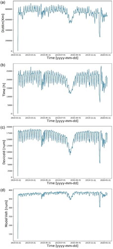
To summarize the sample size, the global VKT and TT, the number of unique device IDs (equivalent to the number of vehicles attributable to the number of users), and the number of unique models were plotted against time. On average, approximately 800,000 km were traveled daily by the monitored vehicles in 25,000 h. The number of vehicles monitored daily was in the range of 10,000 to 20,000 vehicles, among which 150–400 different models can be identified. A cyclic trend was observed in each graph (Figure 1) consisting of a flat section before a high peak, which is immediately followed by a low one. This pattern occurs about 50 times in the 12-month period of analysis, implying that these sequences describe a weekly cycle. The flat section represents weekdays, whereas the two peaks are Friday (high peak) and Sunday (low peak). The low peaks are clear in almost every graph, with consistent observable reductions. The time spent traveling (Figure 1b), and the number of IDs (Figure 1c) decreased by one third and one quarter, respectively, compared to the flat sections. On the other hand, the high peaks are clearer in the distance graph (Figure 1a), when the values increased up to 1,000,000 km, probably due to trips made by commuters. Anomalies are observed in April, August, and December, showing that mobility demand decreased during the Easter Holidays (which fell on 21^st April in 2019, very close to another national holiday, 25^th April), summer holidays (when many residents are not in Turin for the vacation period), and Christmas holidays. The lowest values in each graph were recorded on the weekend before the Christmas holidays (14^th and 15^th December 2019), while Christmas Day ranked as only the 9^th in the classification of the days with lowest distance traveled. Further statistics are collected and reported in the Appendix II.

Figure 1. Daily distance, time, vehicles (IDs) and models of monitored vehicles over the year.

3. Methodology for data analysis and indicator estimation

3.1. Data integration

Additional variables are included to facilitate the extraction of specific information from the dataset. For each trip, its travel time (TT) was computed as the difference between the trip arrival and departure times. Idle times (ITs) were estimated as the difference between the trip arrival time and the following trip departure time, except for each user’s last recorded trip. In that case, the time until the end of the day was reported. ITs were then classified, as will be shown in the next sections, according to their duration, and to the time they take place.

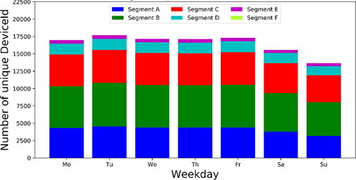
A vehicle classification was also introduced for distinguishing market segments¹ according to vehicle model, as this may provide useful information correlated to vehicle characteristics (energy consumption, battery size, maximum power for charging, etc.), to how the vehicle is used, and to user characteristics to be employed in further analysis. This operation directly follows the simplification of the strings indicating the vehicle model (2.1 Database Structure and Table 3). The association of each vehicle model to its corresponding market segment was performed through the preliminary definition of a data dictionary containing 398 car models. In this phase, trips performed by heavy-duty vehicles, light-commercial vehicles, recreational (RVs) vehicles, and motorbikes, are identified and dropped, reducing the database size (Table 3). Most of the observed vehicles are in the B segment (more than a quarter of the total daily observed on average); the A and C segments include slightly less than a quarter of the vehicles observed; segments D and E include 1 out of 10 and 1 out of 30, respectively, while segment F includes such a low number of vehicles that they cannot even be seen in Figure 2.

Figure 2. Average unique Device IDs observed in each day of the week.

3.2. Detailed travel pattern statistics

Considering that this study has two different main objectives, the analysis can be split into two parts (Tables 4 and 5). First, the detailed travel pattern statistics linked to trip duration, and therefore to battery range, are estimated, mainly in terms of the daily VKT and TT (DVKT and DTT). To consider daily activities instead of single trips is more indicative of the user behavior and is consistent with the hypothesis of one charging operation per day (likely to happen at night at home), already considered in (Jakobsson et al., 2016) and (Khan & Kockelman, 2012) and supported by the fact that private infrastructures have a higher share than public ones (Funke et al., 2019). On the other hand, the cumulative energy consumed after consecutive vehicle activities cannot be considered by only observing single trips. Then, the quantities reported in Table 5 were computed to describe the opportunity for charging vehicle batteries (when and where they are parked). This can provide targeted information to support ECS infrastructure design and development in the city. (1) $$\mathit{DVKT}\left(i,d\right)=\sum _{t\in T\left(d,i\right)}TD\left(i,\mathrm{\hspace{0.17em}}d,\mathrm{\hspace{0.17em}}t\right)$$(1) where $i$ refers to the Device Id, $d$ is the date of trip departure,$\mathrm{ }t$ is the trip, $\Delta t$ is the trip travel time, and $T\left(d,i\right)$ is the set of trips performed by a given ID on a given date. (2) $$IT\left(t_j\right)=d_{ep}\left(i,t_{j+1}\right)-a_{rr}\left(i,t_j\right)$$(2) (3) $$\mathit{CTD}\left(i,d,t_j\right)={\sum }_{t\in T\left(d,i\right):a_{rr}\left(i,d,t\right)<d_{ep}\left(i,d,t_{j+1}\right)}TD\left(i,\mathrm{\hspace{0.17em}}d,\mathrm{\hspace{0.17em}}t\right)$$(3) (4) $$z\left(t_j\right)=z:\mathit{lat}\left(a_{rr}\left(i,t_j\right)\right), \mathit{lon}\left(a_{rr}\left(i,t_j\right)\right)ϵ \partial z$$(4) where $t_j$ and $t_{j+1}$ are two consecutive trips by the same ID, $a_{rr}$ and $d_{ep}$ are arrival and departure times, respectively, of a given trip, $\mathit{lat}$ and $\mathit{lon}$ are the coordinates of arrival or departure, k is the type of IT, z is the zone in which the point characterized by the given $\mathit{lat}$ and $\mathit{lon}$ falls, and $N\left(k,z\right)$ is the number of trips whose arrivals belong to k-class and z-zone.

Table 4. Travel pattern statistics on traveled distances and times.

	Statistics	Description
(1)	DVKT	Daily traveled distance aggregated by Device_ID
(-)	Number of daily trips	Trips performed per day and per Device_ID

Table 5. Travel pattern statistics on idle times.

	Statistics	Description
(2)	Idle Times (ITs)	Time between one trip and the next made by the same ID
(3)	VKT and IT relationship	Cumulative daily VKT by an ID before IT
(4)	ITs Geographical distribution	Map of ITs to be matched with a zoning of Turin MSA

3.3. Idle times definition and classification

Idle times (ITs) are the breaks between one trip and the following one, computed as the time difference between the arrival time and departure time of the i^th trip and the i + 1^th trip, respectively, if performed by the same user (Equation 2(2) $$IT\left(t_j\right)=d_{ep}\left(i,t_{j+1}\right)-a_{rr}\left(i,t_j\right)$$(2) ). For this analysis, the results for each trip are described by the trip information: IT after the trip, cumulative daily VKT, and cumulative daily TT until the beginning of the next IT (including VKT and TT of the last trip made). Moreover, it is worth classifying ITs to understand the needs for charging. Table 6 illustrates the proposed criteria.

Table 6. Idle time classification.

Kind of IT	Abbreviation	Characteristics	Description	Reason of interest
Brief	B	<5 min	Accidental or not interesting breaks	None
Standard	S	>5 min <24 h	Typical break that may occur during daytime	Charging at workplaces, shopping centers, etc.
By-night	N	>5 h <24 h 1:00, 2:00, 3:00, 4:00 or 5:00 AM included	Typical break that may occur at night	Charging at home
Long	L	>24 h	Situation that occurs when vehicle is not used for longer than a day	Vehicle-to-grid strategies

4. Results

4.1. Distribution of traveled distance daily

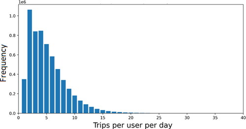
After the dataset cleaning and selection operations, trips were grouped by user and date. The VKT and TT of trips in the same group were summed up, obtaining daily VKT and TT totals. The information about the number of trips is shown in Figure 3. In most cases the number of trips ranged from 1 to 6. Up to 15 trips per day occurred quite often, whereas cases in which an even higher number was recorded were sporadic and may be related to unusual working needs.

Figure 3. Distribution of individual number of daily trips.

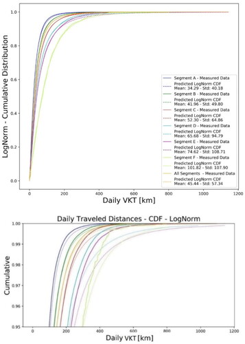
An effort was made to model the experimental cumulative distribution of the daily VKT, by sorting them from the shortest to the longest, and allocating the value of 1 to the longest trip. Figure 4 shows that even in the case of day-level aggregation, the highest number of trips had quite low VKTs, compared to the number of longer trips. For instance, with battery capacity able to guarantee 200, 300 and 400 km, approximately 5%, 2% and 0.1% of daily trips, respectively, could not be achieved across the entire set of observed vehicles. The classification introduced about vehicle segment turns out to be consistent, because the curves are sorted from the lowest to the highest segment. For values over the 40^th percentile of daily traveled distances, the higher the segment is, the longer the distance traveled. Vehicles in segments A and B traveled less than the average, and approximately 99% of the demand observed from the FCD of these segments is already met with a 200 km range. Medium car (segment C) values are just below the average, meaning that C-segmented vehicles need a slightly higher range. As far as concerns the other segments: a 200 km range would satisfy 94%, 92% and 87% of vehicles respectively segmented D, E and F. These percentages increase to 98%, 97% and 95% with a range equal to 300 km and are higher in all the three cases with a range of 400 km. However, it must be specified that the curve for segment F is not as smooth as the others due to the smaller number of vehicles observed. In conclusion, the fact that higher-segmented vehicles rely on more capable batteries is justified by the results observed in terms of distances traveled. The percentage of satisfied car mobility needs can increase and reach almost 99% even with the technological development of batteries to which the market is already subject, especially if the targets are the cars belonging to the segments with higher VKTs.

Figure 4. Log-normal CDFs fitting experimental distribution for different segments (up), with a focus on longer trips (down).

Fitting operations were performed to understand if a statistical distribution can explain the experimental cumulative curve and to uniform the different segment distributions which have a different number of observations, similarly to the operation performed in (Jakobsson et al., 2016). Two main criteria were considered: the probability density function (PDF) associated with the target cumulative density function (CDF) must be positive (traveled distances cannot assume negative values) and have an asymmetrical shape, since short trips are much more recurrent than long ones. According to the exploratory analysis performed, the Log-normal CDFs, once properly fitted, turn out to give an interesting compromise between goodness and conservativity in fitting the experimental curves. The logarithm of traveled distance values shows an almost Gaussian trend (Figure 5). This result is also consistent with the conclusions in (Plötz et al., 2017). Fitting has three targets: ‘loc’ and ‘shape’ parameters refer to the variable transformation (5)(5) $$z=\frac{x-\mathit{loc}}{\mathit{shape}}$$(5) , while ‘s’ refers to the PDF formulation (6)(6) $$f\left(x,s\right)=\frac{1}{sz\sqrt{2\pi }}{e}^{-\frac{{\log }^{2}z}{2s^2}}$$(6) : (5) $$z=\frac{x-\mathit{loc}}{\mathit{shape}}$$(5) (6) $$f\left(x,s\right)=\frac{1}{sz\sqrt{2\pi }}{e}^{-\frac{{\log }^{2}z}{2s^2}}$$(6)

Figure 5. Normal distribution of all daily traveled distance logarithms.

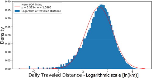
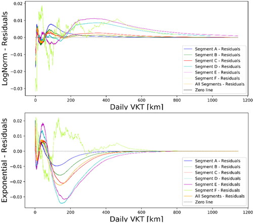
Figure 6. Experimental residuals with respect to Log-normal (up) and Exponential (down) distribution.

Exponential and gamma distributions gave poorer results and are not reported here. Moreover, Weibull distributions do not provide the remarkable results explained in (Plötz et al., 2017), unless they are adopted in the exponentiated form. However, considering the aim of this study, the results for the various distributions have not received focus here as they deserve a specific and deeper analysis.

As shown in Figure 4, the log-normal CDFs provide a satisfactory fit to the experimental curves relative to segments A, B and C, whereas they tend to increase more slowly than those representing segments D, E, and F. Relatively high residuals as shown in Figure 6 observed for short distances are not crucial in this phase, since it is assumed that almost any EV can cover such short distances. Apart from these, the residuals observed in the case of a log-normal CDF (Figure 6a) are:

• almost always positive and lower than 0.5% for the A and B segment curves and for the overall curve (all six segments considered).

• slightly higher (up to 1%) for distances less than 200 km traveled by segment C vehicles.

• approximately equal to 1% for distances greater than 200 km traveled by car segments D and E.

• oscillating for segment F vehicles.

While log-normal CDFs tend to be under the experimental relative curves, exponential and others sometimes go beyond the experimental curves (Figure 6b), and sometimes below. Considering that one of the most crucial limitations to the diffusion of EVs is anxiety about range, log-normal distributions may be a suitable choice among those observed for their precautionary feature. Given a fixed value of distance, the corresponding CDF values are lower than the experimental ones, meaning that a higher percentage of trips has already been covered. Further details about the fitting operations are contained in Appendix III. Results show that log-normal distributions generally lead to lower errors in modeling, except for the MAPE (mean absolute percentage error) (Table C2). This can be justified by the fact that, as aforementioned, those distributions are conservative, and the residuals are almost always positive (the modeled values are higher than those observed).

As final point, it should be mentioned that the shape of the distribution curves is affected by the pattern of mobility demand, which is linked in turn to the geographical area of the trips. Indeed, in Appendix II, several aggregated statistics show that people who travel only out of Turin (‘External’ label) or between Turin and other cities (‘Both’ label) tend to cover a distance which is 3-4 times greater than the one covered by people only moving in Turin (41 and 60 against 15 km, respectively). Travel time is almost twice for users who travel inside and outside Turin boundaries in the same day with respect to the other two classes, which are characterized by similar values of travel time, unlike what happens for what concerns the distances. On the other hand, the number of daily trips does not differ greatly: 4.8, 6.0 and 5.2 daily trips per individual for ‘Internal’, ‘Both’ and ‘External’ classes, respectively.

4.2. Idle times and cumulative traveled distances

Cumulative traveled distances in the day are computed for each vehicle, as well as the idle time duration after the trip to detect if there is a relation between them. For this purpose, only trips whose following IT belongs to the S (Standard) or N (Nocturnal) categories are considered. The probability of an IT of a certain duration after a cumulative traveled distance which falls in a specific range is computed, after having introduced several bins for both the quantities. The bins are 1 hour and 50 km, respectively, in terms of IT duration and cumulative VKT. This computation is aggregated for each car segment, showing similar results in the different cases: an IT shorter than 1 h after a cumulative VKT in the day lower than 50 km occurs in about 40% of the cases regardless of the segment; in about 50% of the trips, the IT and cumulative VKT are lower than 2 h and 100 km, respectively. Also, marginal probabilities are computed (9) for the different distance ranges, to calculate the conditional probability of each IT duration, given the range of cumulative distance (CD). (9) $$\mathit{P}\left(\mathit{IT}\mathrm{|}\mathit{CD}\right)=\frac{\mathit{P}\left(\mathit{IT},\mathit{CD}\right)}{\mathit{P}\left(\mathit{CD}\right)}$$(9)

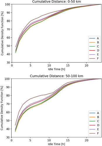
Cumulative distribution can hence be built for each distance range and aggregated by segment, or by cumulative VKT range. Figure 7 shows that IT conditional probability is not greatly affected by the car segment, except for segment F, though its reduced sample size may also have contributed to the result. Nevertheless, the trend in Figure 7 is clear, as the higher the segment is, the higher the curve is on the plot: given an IT duration, lower segments are less likely to perform ITs shorter than that duration, even if this difference is reduced (5% at most). Indeed, for F-segmented cars, the curve is slightly sharper for low values of ITs (less than 3 h), while its slope is lower in the case of high IT values (more than 8 h), reducing the gap with the other curves.

Figure 7. Cumulative distribution of the conditional probability of an IT duration for cumulative daily VKT in the range of 0-50 km and 50-100 km according to the variation of the segment (from A to F).

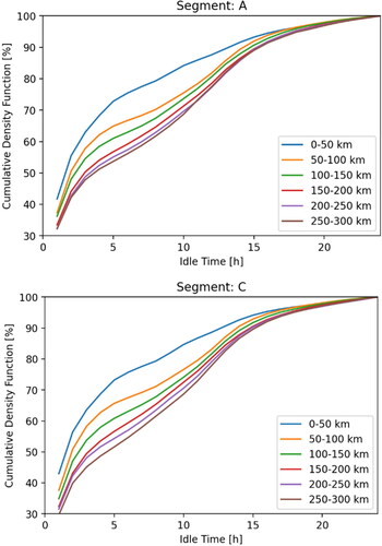
On the other hand, IT conditional probability is sensitive to the cumulative distance range for specific car segments. In Figure 8 the results for segments A and C are reported, since they refer to vehicles with evidently different features and have a good sample size (Figure 2). Given an IT duration, the percentage of vehicles is higher for lower cumulative distances, and the difference between extreme curves is more marked for segment C with respect to segment A (approx. 20% at 5 h).

Figure 8. Cumulative distribution of the conditional probability of an IT duration for segments A and C according to the variation of the cumulative daily VKT range.

4.3. Spatial distribution of idle times

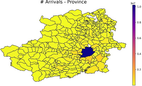
A crucial aspect is to determine which zones of a city would benefit the most from the installation of ECS infrastructure, by evaluating the number of ITs and their mean duration, aggregated by zone. The database contains ITs spread all over the province, but most of them (about 10 million out of 30 million) were recorded in the Turin Municipality (blue area in Figure 9), on which the following analysis will focus.

Figure 9. Number of trip arrivals in the zones of the Metropolitan City of Turin.

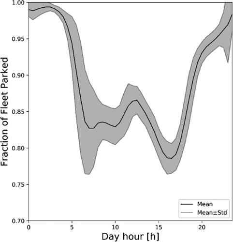
Similarly to (Pearre et al., 2011) and with comparable results, the percentage of the fleet parked is calculated throughout the day. For each thirty-minute period (e.g., 00:30), the number of unused vehicles until the following half an hour (e.g., from 00:30 to 1:00) was computed with respect to the total amount of vehicles used on that day. By averaging the percentages obtained for each day of the year, it is shown in Figure 10 that even in peak hours (morning and late afternoon), approximately 25% of vehicles are traveling. At night, this percentage is lower than 5%.

Figure 10. Percentage of the fleet parked in Turin Municipality: mean and standard deviation.

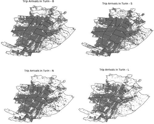
A zonal analysis was performed exploiting a macro zoning² of the Turin Municipality (23 zones), although a further refinement can be easily implemented to catch more detailed information. Each trip arrival coordinates are expressed as a latitude and longitude (WGS84 EPSG:4326). A few points, happening to report Turin as arrival (in the ISTAT column) despite falling outside the shapefile polygons, were dropped. A spatial join operation was performed to determine the area belonging to each point, as shown in Figure 11.

Figure 11. Trip arrivals in Turin. From top-left to bottom-right: brief (B), standard (S), nocturnal (N), and long (L) idle times.

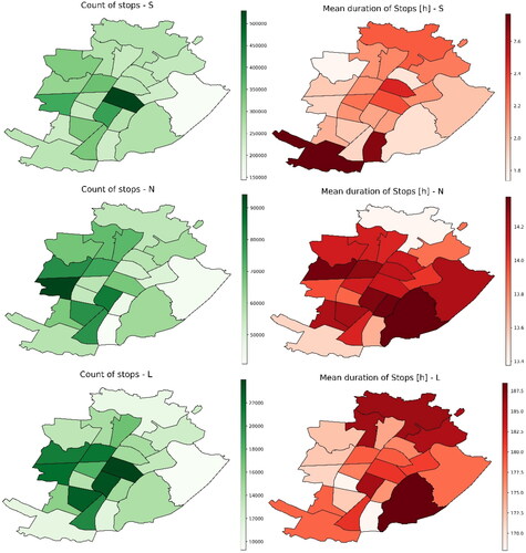
The number of ITs and their mean were calculated with the zone as the aggregation level, after having classified ITs according to previously described criteria (Table 6). Standard breaks that are expected to occur in daytime, are more frequent in the city center (Figure 12a), whereas nocturnal breaks are more uniformly spread especially in residential and peripheral zones (Figure 12c). Considering the IT duration, the city center shows shorter times compared to those observed in many other zones, in respect of both standard ITs (Figure 12b) and nocturnal ones (Figure 12d). Indeed, parking tolls and a nonresidential use of this zone discourages long breaks. On the other hand, standard ITs in peripheral zones (e.g., the southmost zone) are longer due to the presence of factories and other working places. In terms of numerical values, this distinction is clear. The mean of standard IT lasts no longer than 3 hours in each zone, while nocturnal ITs exceed 13-14 h everywhere. ITs longer than 24 h (Figure 12e and f) are supposed to be less systematic and can be useful for the purpose of assessing eventual vehicle-to-grid strategies. Vehicle batteries, in case of long-time parking activities, can be used as storage elements in the grid to compensate for peaks of energy demand. In terms of the number of ITs (Figure 12a, c, e), most daytime ones (approx. 500,000) were recorded in the city center, whereas in other zones generally no more than 300,000 are observed. Nocturnal ITs occur more often in residential zones (up to 100,000 in several zones) rather than in the city center (60,000) or industrial zones (50,000).

Figure 12. ITs count (left) and mean duration (right) at zone level ITs, for different kinds of IT (up to down: standard (S), nocturnal (N), long (L)).

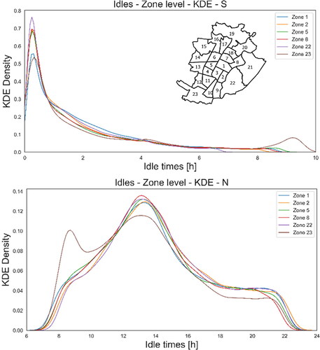
For checking the results in maps (Figure 12b, d, f), the KDE kernel regression curves are plotted for selected zones, which have different characteristics in terms of attraction. For instance, zone 1 represents the city center; zones 2, 5, and 8 are close to the center, but contain many residential areas; zone 22 is a bit further from the city center and consists of mainly residential land used with low population density; zone 23 is supposed to be involved in many work-related trips since many factories are based there. Indeed, zone 23 is the only one in which is shown (Figure 13a) a local peak for 8-hour ITs during the daytime. It is observed, consistently with the map (Figure 12a and b), that in the city center most of standard breaks take place, but they are not as short as those occurring in the other non-peripheric zones. ITs ranging from 1 to 4 h are more likely in the city center, while even shorter ones are more frequent in other residential zones. Standard ITs longer than 4 h have similar density curves, except for zone 23. The mentioned trend is observed for nocturnal ITs as well (Figure 13b). Zones have similar IT density distributions (the map in Figure 12b is dark in almost every non-peripheric zone), except for zone 23, in which a peak of relatively short nocturnal ITs was observed. Combining the spatial distribution of the number of ITs and the duration distributions, it is observed that, given the similar density distribution of short ITs, each zone would ideally require a complete range of power levels. Indeed, short ITs take place everywhere. The power level of ECS can be relatively lower where workplaces, such as factories, are located and should be higher where many maintenance activities (e.g., shopping in small local shops) are performed. On the contrary, the number of ECS per zone increases markedly with the centrality of the zone. Nocturnal IT distribution is quite uniform all over the study area, meaning that each area shows a similar demand both in terms of time availability and number of ITs, except for the zones characterized by an extremely low building density or by the presence of big factories. This demand can be satisfied either by private charging solutions, or by slow public ECS. Longer ITs are not as numerous as those just described for the purpose of this paper and their spatial distribution is not clear.

Figure 13. KDE curves for standard (S) and nocturnal (N) ITs.

5. Conclusions

In this paper passenger car mobility patterns in the Metropolitan City of Turin were extracted and described to assess how compatible they are with the characteristics of electric vehicles (EVs). The mobility patterns were derived from floating car data for 30 million trips, including information on the car maker and model, time, latitude and longitude of departure and arrival, average speed, travel time, and distance traveled. The observation period was the year 2019 and approximately 70,000 km were traveled daily by more than 10,000 (up to 18,000) vehicles every day, comprising 400 different models. Given that no specific information about users and their activities between trips is included in the dataset, this analysis was not aimed at building a demand model for describing user traveling behavior. However, the extended dataset was used to observe car trip-chains for a whole year and detect their relevant features for electric mobility.

The analysis was divided into two parts: studying the distances traveled daily and parking habits. Distances traveled daily are crucial when trying to estimate the percentage of journeys possible with fixed battery ranges, commonly communicated to drivers not only by the energy of the battery, but also through the average distance with a full charge. Parking habits can provide useful information based on real data to identify and classify idle times (ITs) in terms of duration and relate them to the cumulative distance traveled before parking. This analysis can support decisions on the power required for electric charging stations (ECSs) according to the time between trips. Also, relations between zones of the city and local idle times can contribute to assessing where different solutions in terms of ECS number and power level could be better exploited.

On average, a battery range of 200 km would allow about 97% of daily VKT, but it must be emphasized that this percentage varies depending on the vehicle market segment: for mini and small cars (segments A and B) this percentage rises to almost 99%; for medium cars (segment C) the percentage is close to the average (97%); for other segments, this percentage falls to 90%. If the supposed range is extended to 300 km, 95% of daily VKT by F-segmented vehicles are satisfied. Considering an even greater range of 400 km, these percentages no longer differ greatly and increase up to 99%. It was also noted that trip cumulative distribution may be conservatively described by a log-normal cumulative distribution function (CDF).

Parking habits were studied for trips ending in the Turin Municipality (about one third of the total number of trips in the dataset). Idle Times (ITs) were classified according to their type, omitting those shorter than 5 min, to explore different charging infrastructures: daytime ITs may be linked to electric charging stations (ECSs) at workplaces, whereas nocturnal ITs may be linked to home-charging solutions; ITs longer than 24 h may be considered for vehicle-to-grid strategies. Daytime ITs often last no more than 30 minutes and their average duration is about 2 h in most of the zones considered, although in several peripheral zones with industrial land use 8 h ITs can occur. On the other hand, nocturnal ITs are slightly longer in residential zones compared to industrial ones. Most of the daytime ITs were recorded in the city center (approx. 500,000), whereas the count in other zones was generally no more than 300,000.

As expected, nocturnal ITs are more often observed in residential zones (up to 100,000 in several zones) rather than in the city center (approx. 60,000). Long ITs are more unpredictable, since they may be related to irregular parking behaviors, and no trend was detected. Nevertheless, it was observed that they are longer in peripheral residential zones, even if they occur more often in central zones.

Future research will be focused on analyzing patterns according to the day of the week on which trips are performed. An analysis in terms of the energy required by trip and the power provided by the charging infrastructure could extend these results, although more data are required to estimate the energy consumption for the different vehicle types during the various missions accurately. This modeling could include many factors, such as speed/acceleration profiles, vehicle mass and engine size, and road conditions along each route. For this reason, the choice of introducing the vehicle segment classification may be helpful to classify these elements of information.

In addition, no socio-economic data, such as income and household size, about the people traveling was included in this study, due to the lack of information in this regard, and was beyond the scope of this paper. In a further analysis an effort could be made to try and trace back the data presented here to several socio-economic characteristics of the population, starting, for example, with the market segment of the vehicles, supposing that they are typically used by the same person/household.

Acknowledgements

The authors would like to thank the INCIT-EV project³ partners for the profitable discussions on the topics of the project and their valuable comments.

Conflict of interest

On behalf of all authors, the corresponding author states that there is no conflict of interest.

Additional information

Funding

This study is partially supported by the Horizon 2020 INCIT-EV project³, funded by European Union (EU), under the action H2020-EU.3.4. - SOCIETAL CHALLENGES - Smart, Green and Integrated Transport, in which Politecnico di Torino is involved as partner. The dataset exploited in this research was partially purchased with a grant from the European project "Shared mobility opporTunities And challenges foR European citieS" (STARS). Financial support also came through a "Ricerca dei Talenti" grant from Fondazione CRT (DEMONSTRATE project).

Notes

1 Segments defined as in https://en.wikipedia.org/wiki/Euro_Car_Segment, when available.

2 The zoning is performed consistently to that adopted by AMT (Agenzia per la Mobilità Metropolitana di Torino) in which zones are distinguished based on urban districts.

3 Groupe Renault coordinates the INCIT-EV project, to improve the experience of electric vehicle (EV) driving, with a consortium of 33 partners from eight countries (grant agreement No. 875683. https://www.incit-ev.eu/)

4 In this case, the population refers to people older than 10 years

Appendix A:

Turin and its metropolitan area

Results from the IMQ (mobility and transport quality survey) performed by AMM (Agenzia per la Mobilità Metropolitana e Regionale, 2013) about the Metropolitan Statistical Area (MSA) of Turin mobility survey are summarized in Table A1 and Table A2. This survey provides basic information for the Turin conurbation (Turin and 31 other satellite cities). Metropolitan City of Turin (previously known as Turin Province) includes 316 Municipalities.

Table A1. Turin MSA information from AMM survey: population and territory description.

		Conurbation	Turin		Satellite cities
Resident Population	[inhab.]	1,555,518	911,823	59%	643,695	41%
Area	[km^2]	838	130	16%	708	84%
Used Land	[km^2]	227	76	33%	151	67%

Table A2. Turin information from AMM survey: trips and corresponding mean.

		Total	Motorized		Private and Motorized
Conurbation	Trips/day	2,962,000	1,962,000	66%	1,430,000	48%
	Trips/day/person^4	2.11	1.40		1.02

Mobility demand changes during the day, with peaks of approximately 200,000 and 150,000 trips per hour respectively within the 08:00–09:00 and 18:00–19:00 time windows. Private mobility ranges between 70% and 75% during those time intervals and rises to 90% at night, when public transport is less frequent. Maim reasons for the trips are: work (31%), personal shopping (30%), escorting (8%), and study (6%). From origin/destination matrices available, it is observed that slightly less than half the total number of trips using private transport are recorded inside the Turin Municipality. Almost a quarter of those occur between other locations in the conurbation. Places outside the conurbation feature as either the origin or destination in one out of 10 or 20 trips, respectively.⁴

Appendix B:

Preliminary operations with data

Data quality check

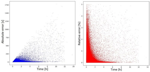
A data quality check was performed to determine if there was any trip with unrealistic or inconsistent VKT, speed or TT values. Time was therefore recomputed as the distance divided by the speed (original values). The speed was recomputed as the distance divided by the time, and the distance was recomputed as the product of the time and speed. Comparisons were made plotting the original versus their relative recomputed entities. All records seem to be consistent, because the points are located extremely close to the 1^st quadrant bisector, in terms of the distance (Figure B1a) and speed (Figure B1b). There were some slight discrepancies in time observed, especially for longer trips (Figure B1c). This is probably related to the method used to estimate the average speed for trips, which may include breaks, making the time longer while keeping the distance constant. The absolute error (Figure B2a) increased with travel time, although only in a small number of instances. The relative error (Figure B2b) was higher for lower values of travel time, and never exceeded 5%, which is consistent with the expected accuracy of speedometers installed in vehicles.

Figure B1. Validation check: provided (x axis) versus computed (y axis) values. Speed (up-left) (a), distance (up-right) (b) and time (bottom) (c).

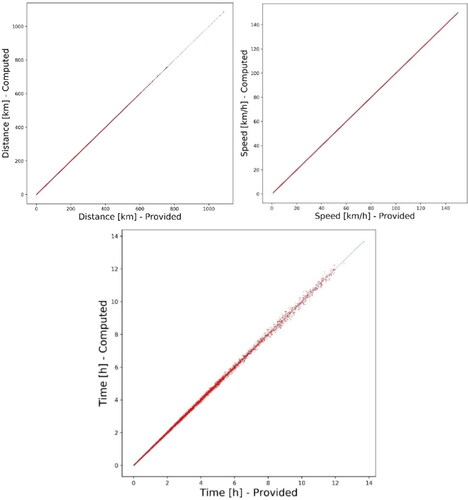
Figure B2. Absolute (left) (a) and relative (right) (b) errors observed comparing provided and computed Travel Time values.

Aggregated statistics

Some aggregated statistics are collected while screening the dataset in Table B1, Table B2, and Table B3). Trips are grouped by date and ID and labeled according to the places involved in the trips. ‘Internal’ and ‘external’ labels respectively mean that all trips performed by a specific ID on a specific date took place inside or outside Turin. ‘Both’ refers to dates when a given ID performs trips both inside and outside Turin.

Table B1. Average Traveled Distance per day per vehicle.

Traveled distance per day per vehicle [km]
Zone		Weekday (Tue-Thu)	Weekend (Sun)
Metropolitan City of Turin (Total)		42.30	50.79
City of Turin	Internal	14.88	12.93
	External	41.10	51.46
	Both	60.34	70.23
Metropolitan Area of Turin	Internal	25.10	22.23
	External	40.27	54.25
	Both	80.95	95.95
Metropolitan City of Turin	Internal	34.11	33.47
	External	123.47	135.60
	Both	121.94	137.71

Table B2. Average Traveled Time per day per vehicle.

Travel time per day per vehicle [h]
Zone		Weekday (Tue-Thu)	Weekend (Sun)
Metropolitan City of Turin (Total)		1.26	1.18
City of Turin	Internal	0.95	0.72
	External	1.07	1.06
	Both	1.76	1.67
Metropolitan Area of Turin	Internal	1.11	0.88
	External	1.00	1.05
	Both	1.85	1.86
Metropolitan City of Turin	Internal	1.18	1.01
	External	1.52	1.66
	Both	2.09	2.15

Table B3. Average Number of trips per day per vehicle.

Number of trips per day per vehicle [#]
Zone		Weekday (Tue-Thu)	Weekend (Sun)
Metropolitan City of Turin (Total)		5.36	4.16
City of Turin	Internal	4.80	3.79
	External	5.16	3.82
	Both	6.03	5.04
Metropolitan Area of Turin	Internal	5.25	4.21
	External	4.99	3.52
	Both	4.97	4.82
Metropolitan City of Turin	Internal	5.49	4.36
	External	1.15	1.08
	Both	4.64	3.85

Appendix C:

Fitting experimental curves

In Table C1 it is shown that the mean and standard deviation of the Log-normal fitted CDF are the closest to the corresponding values of the experimental distribution for segments A, B, and C and of the overall curve. Table 13 shows that the Log-normal CDF often has the lowest error values, except for the MAPE and the MPE. Despite the highest error values and, hence, the lack of accuracy according MPE/MAPE, the sign of MPE is a confirmation that Log-normal fitting is the most conservative one.

Table C1. Absolute variation between computed and experimental distributions in terms of mean and standard deviation (std).

		Δ Mean	Δ Std			Δ Mean	Δ Std
Segment A	LogNorm	2.62%	10.39%	Segment D	LogNorm	6.33%	33.11%
	Weibull	4.69%	17.45%		Weibull	5.08%	12.56%
	Gamma	4.76%	17.50%		Gamma	6.55%	16.36%
	Exponential	3.98%	15.87%		Exponential	9.84%	22.82%
Segment B	LogNorm	1.38%	7.51%	Segment E	LogNorm	7.63%	37.98%
	Weibull	6.27%	20.63%		Weibull	4.02%	9.92%
	Gamma	6.45%	20.91%		Gamma	5.56%	14.01%
	Exponential	5.75%	19.50%		Exponential	9.09%	21.03%
Segment C	LogNorm	2.14%	12.81%	Segment F	LogNorm	3.42%	16.59%
	Weibull	6.34%	18.94%		Weibull	1.72%	5.39%
	Gamma	6.79%	19.93%		Gamma	1.10%	3.35%
	Exponential	6.89%	20.13%		Exponential	1.94%	4.15%
All Segments	LogNorm	1.49%	9.57%
	Weibull	7.26%	22.15%
	Gamma	7.80%	23.35%
	Exponential	8.24%	24.21%

Table C2. Fit accuracy in terms of (from left to right): mean absolute error (MAE), mean square error (MSE), root mean square error (RMSE), mean absolute percentage error (MAPE), mean percentage error (MPE), and R² score.

		MAE	MSE	RMSE	MAPE	MPE	R2
Segment A	LogNorm	0.003835	0.000025	0.004962	19.751299	−18.452474	0.999705
	Weibull	0.004239	0.000025	0.005045	3.691687	2.502451	0.999695
	Gamma	0.003972	0.000023	0.004791	3.248378	2.162947	0.999725
	Exponential	0.004461	0.000028	0.005323	4.441980	3.155158	0.999660
Segment B	LogNorm	0.003258	0.000018	0.004199	18.965016	−17.837976	0.999788
	Weibull	0.005054	0.000041	0.006416	4.158289	2.709758	0.999506
	Gamma	0.004765	0.000039	0.006205	3.642227	2.288951	0.999538
	Exponential	0.005274	0.000043	0.006541	4.715672	3.205130	0.999487
Segment C	LogNorm	0.002553	0.000011	0.003352	16.485184	−15.520633	0.999865
	Weibull	0.006367	0.000061	0.007814	4.882112	3.057496	0.999267
	Gamma	0.006329	0.000063	0.007918	4.518913	2.721878	0.999248
	Exponential	0.006295	0.000063	0.007922	4.370925	2.578064	0.999247
Segment D	LogNorm	0.001861	0.000008	0.002792	11.047410	−10.364844	0.999906
	Weibull	0.007899	0.000089	0.009425	6.063979	3.639182	0.998934
	Gamma	0.008979	0.000116	0.010771	6.245090	3.466566	0.998608
	Exponential	0.011078	0.000194	0.013928	4.232291	−0.768726	0.997672
Segment E	LogNorm	0.002599	0.000012	0.003479	8.396056	−7.645315	0.999855
	Weibull	0.008803	0.000103	0.010126	6.720184	3.848348	0.998770
	Gamma	0.010067	0.000133	0.011536	6.931337	3.646580	0.998403
	Exponential	0.012490	0.000224	0.014965	4.584167	−0.822816	0.997313
Segment F	LogNorm	0.008605	0.000114	0.010666	17.968495	−15.193055	0.998635
	Weibull	0.005577	0.000046	0.006793	3.563632	0.369103	0.999446
	Gamma	0.005653	0.000047	0.006888	3.745261	−1.707067	0.999431
	Exponential	0.009259	0.000120	0.010961	5.706947	3.837073	0.998558
All Segments	LogNorm	0.002595	0.000012	0.003448	17.845070	−16.870298	0.999857
	Weibull	0.006181	0.000059	0.007693	4.814132	3.014647	0.999290
	Gamma	0.006257	0.000063	0.007927	4.511944	2.686623	0.999246
	Exponential	0.006150	0.000064	0.008030	3.930650	2.136056	0.999226

References

- ACI, CNR-DIITET, Fondazione Filippo Caracciolo, ENEA (Eds.), (2019). Per una transizione energetica eco-razionale della mobilità automobilistica.
- Agenzia per la Mobilità Metropolitana e Regionale, (2013). IMQ2013_RapportoSintesi.pdf.
- Anderson, J. E., Lehne, M., & Hardinghaus, M. (2018). What electric vehicle users want: Real-world preferences for public charging infrastructure. International Journal of Sustainable Transportation, 12(5), 341–352. https://doi.org/10.1080/15568318.2017.1372538
- Arslan, O., Yıldız, B., & Ekin Karaşan, O. (2014). Impacts of battery characteristics, driver preferences and road network features on travel costs of a plug-in hybrid electric vehicle (PHEV) for long-distance trips. Energy Policy, 74, 168–178. https://doi.org/10.1016/j.enpol.2014.08.015
- Associazione Nazionale Filiera Industria Automobilistica – ANFIA. (2020). FOCUS ITALIA MERCATO AUTOVETTURE.
- Axsen, J., & Kurani, K. S. (2013). Hybrid, plug-in hybrid, or electric—What do car buyers want? Energy Policy, 61, 532–543. https://doi.org/10.1016/j.enpol.2013.05.122
- Brenna, M., Foiadelli, F., Leone, C., & Longo, M. (2020). Electric vehicles charging technology review and optimal size estimation. Journal of Electrical Engineering & Technology, 15(6), 2539–2552. https://doi.org/10.1007/s42835-020-00547-x
- Chen, T., Zhang, X.-P., Wang, J., Li, J., Wu, C., Hu, M., & Bian, H. (2020). A review on electric vehicle charging infrastructure development in the UK. Journal of Modern Power Systems and Clean Energy, 8(2), 193–205. https://doi.org/10.35833/MPCE.2018.000374
- Dalla Chiara, B., Deflorio, F., & Eid, M. (2019). Analysis of real driving data to explore travelling needs in relation to hybrid–electric vehicle solutions. Transport Policy, 80, 97–116. https://doi.org/10.1016/j.tranpol.2018.04.009
- Danielis, R., Giansoldati, M., & Rotaris, L. (2018). A probabilistic total cost of ownership model to evaluate the current and future prospects of electric cars uptake in Italy. Energy Policy, 119, 268–281. https://doi.org/10.1016/j.enpol.2018.04.024
- Dong, J., Liu, C., & Lin, Z. (2014). Charging infrastructure planning for promoting battery electric vehicles: An activity-based approach using multiday travel data. Transportation Research Part C: Emerging Technologies, 38, 44–55. https://doi.org/10.1016/j.trc.2013.11.001
- Duoba, M., & Fernandez Canosa, A. (2019). Mesoscopic Approach to Modeling Electric Vehicle Fleets based upon Driving Activity Data to Investigate Recharge Strategies’ Impact on Grid Loads [Paper presentation]. 2019 IEEE Transportation Electrification Conference and Expo (ITEC). Presented at the 2019 IEEE Transportation Electrification Conference and Expo (ITEC), pp. 1–6. https://doi.org/10.1109/ITEC.2019.8790617
- Egbue, O., & Long, S. (2012). Barriers to widespread adoption of electric vehicles: An analysis of consumer attitudes and perceptions. Energy Policy, 48, 717–729. https://doi.org/10.1016/j.enpol.2012.06.009
- Franke, T., & Krems, J. F. (2013). What drives range preferences in electric vehicle users? Transport Policy, 30, 56–62. https://doi.org/10.1016/j.tranpol.2013.07.005
- Funke, S. Á., Sprei, F., Gnann, T., & Plötz, P. (2019). How much charging infrastructure do electric vehicles need? A review of the evidence and international comparison. Transportation Research Part D: Transport and Environment, 77, 224–242. https://doi.org/10.1016/j.trd.2019.10.024
- Greaves, S., Backman, H., & Ellison, A. B. (2014). An empirical assessment of the feasibility of battery electric vehicles for day-to-day driving. Transportation Research Part A: Policy and Practice, 66, 226–237. https://doi.org/10.1016/j.tra.2014.05.011
- Hu, L., Dong, J., Lin, Z., Yang, J. (2018). Analyzing battery electric vehicle feasibility from taxi travel patterns: The case study of New York City, USA. Transportation Research Part C: Emerging Technologies, 87, 91–104. https://doi.org/10.1016/j.trc.2017.12.017
- Jakobsson, N., Gnann, T., Plötz, P., Sprei, F., & Karlsson, S. (2016). Are multi-car households better suited for battery electric vehicles? – Driving patterns and economics in Sweden and Germany. Transportation Research Part C: Emerging Technologies, 65, 1–15. https://doi.org/10.1016/j.trc.2016.01.018
- Jenn, A., Laberteaux, K., & Clewlow, R. (2018). New mobility service users’ perceptions on electric vehicle adoption. International Journal of Sustainable Transportation, 12(7), 526–540. https://doi.org/10.1080/15568318.2017.1402973
- Khan, M., & Kockelman, K. M. (2012). Predicting the market potential of plug-in electric vehicles using multiday GPS data. Energy Policy, 46, 225–233. https://doi.org/10.1016/j.enpol.2012.03.055
- Kopp, J., Gerike, R., & Axhausen, K. W. (2015). Do sharing people behave differently? An empirical evaluation of the distinctive mobility patterns of free-floating car-sharing members. Transportation, 42(3), 449–469. https://doi.org/10.1007/s11116-015-9606-1
- Krupa, J. S., Rizzo, D. M., Eppstein, M. J., Brad Lanute, D., Gaalema, D. E., Lakkaraju, K., & Warrender, C. E. (2014). Analysis of a consumer survey on plug-in hybrid electric vehicles. Transportation Research Part A: Policy and Practice, 64, 14–31. https://doi.org/10.1016/j.tra.2014.02.019
- Lindsey, M., Schofer, J. L., Durango-Cohen, P., & Gray, K. A. (2011). The effect of residential location on vehicle miles of travel, energy consumption and greenhouse gas emissions: Chicago case study. Transportation Research Part D: Transport and Environment, 16(1), 1–9. https://doi.org/10.1016/j.trd.2010.08.004
- Pagany, R., Camargo, L. R., & Dorner, W. (2019). A review of spatial localization methodologies for the electric vehicle charging infrastructure. International Journal of Sustainable Transportation, 13(6), 433–449. https://doi.org/10.1080/15568318.2018.1481243
- Pearre, N. S., Kempton, W., Guensler, R. L., & Elango, V. V. (2011). Electric vehicles: How much range is required for a day’s driving? Transportation Research Part C: Emerging Technologies, 19(6), 1171–1184. https://doi.org/10.1016/j.trc.2010.12.010
- Plötz, P., Jakobsson, N., & Sprei, F. (2017). On the distribution of individual daily driving distances. Transportation Research Part B: Methodological, 101, 213–227. https://doi.org/10.1016/j.trb.2017.04.008
- Schneider, F., Ton, D., Zomer, L.-B., Daamen, W., Duives, D., Hoogendoorn-Lanser, S., & Hoogendoorn, S. (2021). Trip chain complexity: a comparison among latent classes of daily mobility patterns. Transportation, 48(2), 953–975. https://doi.org/10.1007/s11116-020-10084-1
- Suganya, S., Charles Raja, S., & Venkatesh, P. (2017). Smart management of distinct plug-in hybrid electric vehicle charging stations considering mobility pattern and site characteristics. International Journal of Energy Research, 41(14), 2268–2281. https://doi.org/10.1002/er.3788
- Sun, X.-H., Yamamoto, T., & Morikawa, T. (2015). Charge timing choice behavior of battery electric vehicle users. Transportation Research Part D: Transport and Environment, 37, 97–107. https://doi.org/10.1016/j.trd.2015.04.007
- Sun, X.-H., Yamamoto, T., Takahashi, K., & Morikawa, T. (2018). Home charge timing choice behaviors of plug-in hybrid electric vehicle users under a dynamic electricity pricing scheme. Transportation, 45(6), 1849–1869. https://doi.org/10.1007/s11116-018-9948-6
- Tamor, M. A., Gearhart, C., & Soto, C. (2013). A statistical approach to estimating acceptance of electric vehicles and electrification of personal transportation. Transportation Research Part C: Emerging Technologies, 26, 125–134. https://doi.org/10.1016/j.trc.2012.07.007