Bicycle streetscapes: a data driven approach to mapping streets based on bicycle usage

Abstract

Cities are making infrastructure investments to make travel by bicycle safer and more attractive. A challenge for promoting bicycling is effectively using data to support decision making and ensuring that data represent all communities. However, ecologists have been addressing a similar type of question for decades and have developed an approach to stratifying landscapes based on ecozones or areas with homogenous ecology. Our goal is to classify street and path segments and map streetscape categories by applying ecological classification methods to diverse spatial data on the built environment, communities, and bicycling. Piloted in Ottawa, Canada, we use GIS data on the built environment, socioeconomics and demographics of neighborhoods, and bicycling infrastructure, behavior, and safety, and apply a k-means clustering algorithm. Each street or path, an intuitive spatial unit that reflects lived experience in cities, is assigned a streetscape category: bicycling destination; wealthy neighborhoods; urbanized; lower income neighborhoods; and central residential streets. We demonstrate how streetscape categories can be used to prioritize monitoring (counts), safety, and infrastructure interventions. With growing availability of continuous spatial data on urban settings, it is an opportune time to consider how street and path classification approaches can help guide our data collection, analysis, and monitoring. While there is no one right answer to clustering, care must be taken when selecting appropriate input variables, the number of categories, and the correct spatial unit for output. The approach used here is designed for bicycling application, yet the methods are applicable to other forms of active transportation and micromobility.

Keywords:

• Bicycle counts
• bicycling
• exposure
• regionalization
• Strava

1. Introduction

To support policies that help achieve sustainability targets by increasing bicycling, cities need data for planning and monitoring. Recent technical advances mean that there are extensive and diverse data available in cities to support planning, including data about people (e.g., the census), the built environment (e.g., road networks, and crowdsourced reports on safety and infrastructure), and bicycling behavior (e.g. traditional count programs and spatially and temporally continuous count data from apps) (Nelson et al., 2021a) An emerging challenge is making practical use multiple dimensions of data to support human decision making in planning, and it is particularly challenging but important to ensure that spatial data are collected in a way that represents all communities (Nelson et al., 2022).

As an example of this challenge, there has been a surge of interest in building and deploying robust bicycle counting programs (Brown et al., 2021; Lee & Sener, 2021). With bicycle count data, policy makers are better able to justify where and when to make infrastructure investments and can monitor the impact of pro-bicycling policies (Boss et al., 2018). As well, bicycle counts are important for addressing safety issues, which is needed to overcome barriers to more people using bikes (Winters et al., 2011). With ridership data, safety evaluations can include measures of exposure, or the number of bicycling trips. Without exposure data, safety issues tend to be associated with areas of high bicycling ridership rather than other issues such as poor urban design (Ferster et al., 2021).

As cities sharpen their focus on designing and deploying robust bicycle count programs, the question of where to install bicycle counters has arisen as a practical problem for city planners (Brum-Bastos et al., 2019). Bicycle counts are frequently collected by deploying temporary counters, using either temporary equipment (e.g., pneumatic tubes or cameras) or people to conduct counts, or by using permanent counters to measure continuously at a single location. Permanent counters provide data on the number of bicyclists that pass by a location at very high temporal resolutions (i.e., 15-minute intervals) and can determine direction of travel. The quality of permanent counter data combined with the development of data dashboards and visualizations have made having a network of permanent counters an ideal approach for robust bicycling ridership data collection. However, the cost of permanent counters is not trivial, and transportation planners must optimize the locations of counters to ensure data provide a representative overview of bicycling levels and changes throughout a city. Often permanent counters are in ideal bicycling locations to demonstrate trips as returns on infrastructure investments; starting discussions about representation are important to ensure the equitable sharing of bicycling infrastructure investments (Agyeman & Doran, 2021). Incorporating data about people and the built environment in designing count programs could help to evaluate and improve the representation and efficiency of bicycle count programs. Further, delineating categories makes it easier to discuss safety (Ferster et al., 2021), optimize data collection (Brum-Bastos et al., 2019), and to discuss who has access to high quality bicycling infrastructure (Boss et al., 2018).

The growing availability of spatial data on urban environments (Nelson et al., 2021a) creates an opportunity to leverage methods from ecology to stratify landscapes for systematic sampling, including the systematic siting of bicycle count locations. Regionalization, or spatial classification, is the grouping of geographical entities into categories based on similarity of properties or relationships (Chorley & Haggett, 1967; Johnston, 1968). Regionalization schemes often rely on clustering approaches. Clustering is a type of unsupervised classification used to identify natural patterns and structure by partitioning observations into subsets (or groups) using statistical distance measures of attributes and is capable of considering multiple variables simultaneously. Clustering algorithms group observations so that groups have similar attributes, and observations in different groups have dissimilar attributes. Clustering is an important step in exploratory data analysis in many fields because it can organize unstructured datasets into sensible groups (Ghosal et al., 2020; Omran et al., 2007).

Regionalization schemes exist at a range of scales including ecozones and ecoregions that commonly delineate areas with similar vegetation, soils, elevation, and climate (e.g., Riitters et al., 2002; Wulder et al., 2008). These regions can be used to monitor rates of disturbance (e.g., forest harvesting, wildfire, and land use change) (White et al., 2017), the representation of parks and protected areas (Andrew et al., 2014), and inform regional management strategies (Schultz, 2005). Ecological classifications can occur at a range of scales and resolutions using similar methods, from broad ecozones that delineate zones within nations, to much more detailed classifications within individual forest stands to delineate wetlands based on topography, vegetation, and soils based on high-spatial resolution aerial photographs (Meidinger & Pojar, 1991). Ecozones have proven a practical spatial unit for stratifying sampling (Graef et al., 2005), delineating study areas (Hargrove & Hoffman, 2004), and monitoring change through time (Fitterer et al., 2012; Wulder et al., 2011). In recent years, ecologists have used spatially continuous satellite data to map ecozones and have regionalized urban environments to monitor ecology (Schneider et al., 2010); similar approaches have been used to reduce uncertainty in the census for minority groups (Spielman & Folch, 2015).

Data analogous to continuous data used by ecologists to define ecozones is available in the bicycling realm, from fitness apps, such as Strava, which provide continuous space time data on observed ridership behavior. Though demographically biased toward app users, in cities with high app usage the patterns of Strava bicycling correlate with the spatial patterns for all bicycling ridership (Nelson et al., 2021b). Furthermore, because data are collected across all space it can be used as input into clustering algorithms similar to those used by ecologists to delineate ecozones. Additionally, Strava can be combined with a growing number of other bicycling relevant data sets, such as bicycling infrastructure and built environment data from OpenStreetMap (OSM) (Ferster et al., 2020) and crowdsourced data on bicycling safety (Nelson et al., 2021a), which provide data about roads, land use, amenities, and safety.

Our goal is to map streetscape categories by applying ecological classification methods for delineation of ecoregions to diverse spatial data on the built environment, communities, and bicycling and highlight how they can be used for prioritizing bicycling safety and promotion interventions. We demonstrate an approach to classify street segments, an intuitive spatial unit that reflect how people experience cities, using variables that are relevant for current bicycling research. Streetscape categories are useful for stratifying cities to identify locations of bicycle counts. As well, streetscape categories provide a spatial unit that can be used for monitoring bicycling ridership trends, impacts of policy and investments, and provide a spatial framework for monitoring changes in bicycling ridership, infrastructure, and safety.

2. Study area

We used the City of Ottawa, Canada in 2016 as a case study to demonstrate the approach. The year 2016 is a useful baseline given it is the date of the census and coincides with an outreach campaign that the city undertook to increase Strava use by all bicyclists. Ottawa has a population of 934,243, and in area covers a wide range of land uses from urban (downtown) to rural areas (in less central locations) (Statistics Canada, 2016). Approximately 2.6% of workers commuted by bicycle as their primary mode of travel to work across the census subdivision (Statistics Canada, 2016). The region has invested significant financial resources in bicycle and multi-use infrastructure over the past several years and currently has over 600 km of bicycle paths (National Capital Commission, 2017). Infrastructure that we monitor for change in ridership patterns: are Adawe bike and pedestrian bridge (opened December 2015), Hickory bike and pedestrian bridge (opened August 2015), MacDonald-Cartier pathway (opened December 2015). Within the City of Ottawa, we selected a study area that fell within 3 km of the Rideau Canal and Trillium Line multi-use path, encompassing the city center and nearby neighborhoods to demonstrate an approach that can be scaled to other places and extents.

3. Data

To define streetscape categories, we used data on a number or variables known to impact bicycle ridership (Buehler & Dill, 2016). We separate these into three categories: 1) built environment; 2) socioeconomics and demographics; and 3) bicycling infrastructure, behavior, and safety (Table 1). Variables are mapped to the spatial unit of the street segments which, we obtained from OpenStreetMap.org (OSM). To attribute the variables to the street segments, for points and polygons representing the built environment we measured nearest neighbor distance to the street segment (i.e., the shortest distance to any point on the street segment). Line data were directly attributed to each street segment. For other polygon data, the approach for each variable is described below.

Table 1. List of variables and their operationalization along with data sources.

Group	Variable	Operationalization	Data Source
Built Environment	bus_dist	Distance (m) to nearest bus stop	OpenStreetMap highway = bus_stop
	commercial_retail_perc	% of commercial and retail centers within a 30 m buffer of a street segment	OpenStreetMap landuse = [commercial, retail]
	natural_dist	Distance to nearest park, natural land use, or water.	OpenStreetMap natural = * OR leisure = park OR waterway = *
	parking_dist	Distance (m) to nearest motor vehicle parking	OpenStreetMap amenity = parking
	shopping_entertainment_dist	Distance (m) to nearest entertainment and shopping centers	OpenStreetMap shop=* OR amenity = [bar, cinema, cafe, restaurant, fast_food]
Socioeconomic &Demographic	indigenous_perc	% of total population that is indigenous	Canadian Census total aboriginal identity in the population / the total population
	income_med	Median income	Canadian Census median income of economic families in 2015
	minorities_perc	% of total population that belong to visible minority groups	Canadian Census total visible minority population / the total population
	pop_dens	Population density	Canadian Census population density per square kilometer
Bicycling Infrastructure, Behavior, & Safety	bike_mode_share	Bicycle mode share	Canadian Census main mode of travel to work for the working population aged 15 or older / the working population aged 15 or older who commute to work
	Can_BICS	Bike infrastructure comfort class, no infrastructure or non-conforming, low (painted lanes on busy roads), medium (multi-use paths), or high (cycle tracks, bike paths, and local street bikeways).	City of Ottawa open data
	incident_dist	Distance (m) to nearest bike incident	BikeMaps.org, Ottawa police dept.
	Strava_commute_perc	% of activities classified as commutes.	Strava Metro
	Strava_trip_count	Mean daily Strava trips on a street segment on summer weekdays	Strava Metro

3.1. Built environment

Individual bicycling behavior is known to be influenced by land use and the built environment (Cui et al., 2014; Winters et al., 2010). Built environment variables we used in this analysis included the distance to the nearest bus stop, a measure of land use represented as the percentage of commercial centers within 30 m buffer, the distance to the nearest natural area or park, distance to the nearest parking lot, and the distance to nearest shopping or entertainment center. These data were acquired by querying OSM using the R package osmdata (Padgham et al., 2017). These features were represented by both points and polygons, depending on mapping convention on OSM. For many variables we calculated the nearest distances to minimize the use of arbitrary thresholds. However, we did calculate an areal measure of land use, measured as the % of land area used for commercial and retail land use within a 30 m buffer area of the road centerline. This buffer distance was a practical and theoretical value selected to capture most of the buildings facing a street without overlap between blocks in the densest parts of the city. Related to this category, is bicycling infrastructure, described in the Bicycling Infrastructure, Behavior, & Safety section below.

3.2. Socioeconomic and demographic

Bicycling ridership is also known to vary based on income and race (Lubitow et al., 2019). We are particularly interested in transportation services for Indigenous communities and other racial minorities given that such communities are underserved with respect to active transportation infrastructure (Lubitow et al., 2019), so using data from the Canadian Census we calculated the percent of the total population who are 1) Indigenous; and 2) visible minorities. We used median household income as an area-level measure of socioeconomic status. We also used population density because it is strongly related to urban form. To map the census areal unit to a street segment we calculated the area weighted mean of the value within dissemination areas within a 200 m buffer (since streets are often the boundaries for dissemination areas); for example, if a street was located equally between two dissemination areas, the mean value of the two would be assigned. We chose 200 m as a comfortable walking distance that represents the immediate surroundings of a street segment. We used the R package cancensus (von Bergmann et al., 2021) to obtain census data, and the function st_interpolate_aw from the package sf (Pebesma, 2018) to calculate area weighted means.

3.3. Bicycling infrastructure, behavior, and safety

Using data from multiple sources, we included six variables on bicycling infrastructure, behavior, and safety. First, we used the Canada Census journey to work bicycle mode share using the same methods as the other census variables. To characterize bicycling infrastructure, we classified 2016 bicycle infrastructure data from the City of Ottawa into three bicycling comfort classes following the Canadian Bikeway Comfort and Safety Classification System (Can-BICS) (Winters et al., 2020). High comfort infrastructure includes cycle tracks and bike paths that are separated from other modes. Medium comfort infrastructure includes multi-use paths that are shared with pedestrians. Low comfort infrastructure includes painted lanes with no physical separation from motorized traffic. Shared lanes on major roads (i.e., sharrows) and painted shoulders were not included since they do not improve safety compared to no infrastructure (Teschke et al., 2014, TAC, 2020, Ferenchak & Marshall, 2016). The Can-BICS variable incorporates the number of lanes and traffic diversion as an indicator of motorized vehicle volumes, speeds, and road function suitable for all-ages-and-abilities bicycling, similar to the variables used in more traditional street classifications (e.g., number of lanes, speed limit, volume, and functional class) (Forbes, 1999), but focused on all-ages-and-abilities bicycling.

Real and perceived concerns about bicycling safety are a primary barrier to people bicycling (Winters et al., 2011). For safety we used self-reported safety incidents from BikeMaps.org (Nelson et al., 2015; Laberee et al., 2021; n = 158) and police records of bicycling safety incidents from Ottawa open data (City of Ottawa 2020; n = 740) for the years 2015 and 2016, matching the Strava bicycling behavior data and census data. For each street segment, we calculated the nearest-neighbor distance to the closest incident. To summarize safety, post-classification, we counted the number of incidents within a 15 m buffer (intended to cover a typical roadway width from the centerline) of each streetscape category and the full study area.

Bicycle behavior, which we consider both the purpose and frequency of bicycle trips, was represented using Strava data. Strava is a fitness app that bicyclists use to track rides. Data are compiled and shared by Strava Metro to support active transportation planning. From Strava we used data on the total number of bicyclists by street segment and the trip purpose. Trip purpose can be commute or recreation. While it is possible for Strava users to set the trip purpose, most often it is not consistently labeled and as such Strava has a classification algorithm that they use to label commute trips based on patterns in bicycling. While Strava is used most commonly by recreational bicyclists, it has been shown to correlate well with all bicycling, especially in urban areas correlates (Jestico et al., 2016). In Ottawa, we expect a higher proportion of commuters than typical in Strava data due to a marketing campaign led by the city for commuters to contribute data to Strava in advance of acquiring the data.

4. Methods

We used the street network provided by Strava Metro (originally sourced from OpenStreetMap) and extracted the attributes to street segments—the length of street, paths, and trails between two intersections. The street segments had a mean length 100 m, with a standard deviation of 107 m, and ranging from 1 m to 2 km. We created a data matrix combining all attributes listed in Table 1. The ordinal categorical variable (Can-BICS class: no infrastructure, low, medium, and high comfort) was represented by integers from 0 to 3 (assuming monotonically increasing steps between the classes). To compare variables with different units and scales, we scaled all variables using the R function “scale” to divide each value by the root mean square of the variable to produce positive scaled values. We used a correlation matrix to check for collinearity and found that the Pearson correlation coefficient was less than 0.7 for all variables. K-means clustering is an unsupervised classification approach that aims to partition the data so that intra-cluster similarity is high and the inter-cluster similarity is low. We generated streetscape categories using the R function “kmeans” with default parameters. To determine the optimum number of clusters, we used the elbow method by plotting the within-cluster sum of squares from k = 1 to 20 and selected the value of k where the rate of change in the within-cluster sum of squares started to diminish. While methodologically we are using a clustering algorithm, the way we are conceptualizing the application of the clustering algorithm is to delineate streets into categories representative of bicycling behavior, and for the remainder of the paper use the term category synonymous with cluster. We named the streetscape categories by comparing means and distributions for the different regions and by viewing street-level imagery.

5. Results

The study area compared 1,215 km of street segments and trails. Based on the evaluation of an elbow plot, the k-means clustering resulted in classification into five streetscape categories, or groups of street segments with similar built environment, socioeconomics and demographics, bicycling behavior, infrastructure, and safety characteristics (Figure 1).

Figure 1. The Ottawa streetscape categories. Basemap tiles by Stamen Design, under CC BY 3.0. Data by OpenStreetMap, under ODbL.

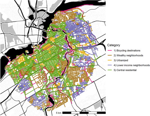
Streetscape category 1 represents bicycling destinations. It includes higher-than-average proportions of bicycling infrastructure - mostly medium-comfort multi-use paths (89.5%) (Table 2). The bicycling destinations category is closer to natural features than the other categories, while further than average to shopping and entertainment, and commercial and retail, and incomes are higher than average (Figure 2). This category has the most Strava activities, while incidents per kilometer or per trip are less than half of category 3 (Figure 3). The bicycling destinations region is often located along rivers and canals.

Figure 2. Distributions by street segment (n = 12,170, 1,215 km) for the variables used to classify streetscape category. Scaled values are shown to compare multiple units. Note varying x axis.

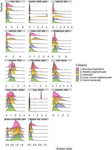
Figure 3. Bubble chart showing how the incidents normalized by street length varies with the number of Strava riders for each streetscape category. The bubble number lists the category and the size of the bubble represents the total length in kilometers.

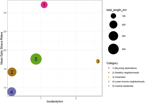
Table 2. Summary of the geometry, length-weighted means (for continuous variables), and proportions (for categorical variables) for the streetscape category.

Variable type	Variables	Type (unit)	Streetscape category
			Bicycling destinations	Wealthy neighborhoods	Urbanized	Lower income neighborhoods	Central residential	Study Area
Geometry	Length	kilometers	143	263	87	262	459	1,215
	Length	% of study area	12	22	7	22	38	100
Built Environment	bus_dist	meters	183	223	58	91	78	123
	comm_retail_perc	%	3	0	75	4	5	8
	natural_dist	meters	17	83	150	112	66	80
	parking_dist	meters	86	178	21	49	50	80
	shop_ent_dist	meters	290	566	101	181	152	260
Socioeconomic & Demographics	indigenous_perc	%	2	2	2	4	2	3
	income_med	$	119,029	148,287	103,811	80,637	113,014	113,712
	minorities_perc	%	20	16	24	31	20	22
	pop_dens	people / km^2	2,538	2,077	4,168	3,868	4,569	3,610
Bicycling Infrastructure, Behavior, & Safety	bike_mode_share	%	8	8	6	4	9	7
	incident_dist	meters	309	532	286	626	202	384
	Can-BICS low comfort	% of category	7.5	1.3	3.6	2.5	4.9	3.8
	Can-BICS medium comfort	% of category	89.5	0	0.5	0	0	10.6
	Can-BICS high comfort	% of category	3	0	0	0	0	0.4
	Strava_commute_perc	%	54	44	56	52	57	53
	Strava_trip_count	count	35	13	16	9	16	16

Streetscape category 2 represents wealthy neighborhoods. The high-income category has the lowest access to amenities such as public transportation, parking, commercial and retail, and shopping and entertainment. It also has the smallest percentage of the total population belonging to visible minority groups, and the lowest population density of all the regions. It is nearer than average to natural areas. Compared to the other categories, it has very few safety incidents per kilometer, The wealthy neighborhoods region is often located in less central areas, and often near water bodies.

Streetscape category 3 represents urbanized. It has the best access to public transportation, shopping and entertainment, and commercial and retail. It has the highest average population density, but the distribution was bimodal, with some streets having very high population densities (where apartments are located), and some streets having very low population densities (e.g., where office buildings are located). It had the highest journey to work by bicycle mode share. It had slightly lower than average incomes. It has the second highest Strava activity, and the highest percentage of Strava commute trips. The urbanized region has the highest rate of incidents per kilometer. This region is located in central locations (i.e., downtown), and in other patches and corridors across the city.

Streetscape category 4 represents lower income neighborhoods. This category has better than average access to public transportation and motor vehicle parking and is mostly served by low comfort bike infrastructure (painted lanes) and has better than average access to shopping and entertainment. Compared to the other categories, category 4 had the lowest median household income, the highest proportion of Indigenous population and the highest proportion of visible minority populations, less access to natural areas, and the lowest bike mode share. While category 4 had lower average population density, the distribution had a long tail, meaning that some streets were suburban with single family houses, while other had apartment blocks and higher population density. Category 4 had a low rate of bike incidents, but it also had very few trips recorded on Strava. Category 4 was located on the periphery of the study area.

Streetscape category 5 represents central residential. Category 5 was similar to category 4, but with higher incomes, a lower percentage the population who are Indigenous, a lower percentage the population belonging to visible minorities, and higher than average population density. Category 5 had a similar number of incidents per kilometer as category 1, but it had fewer Strava trips. Category 5 was in central areas near adjacent to all other clusters.

6. Discussion

Applying ecological theory to urban environments is not new, yet changes in data and new management questions makes it beneficial to revisit how regionalization approaches can support data needs in cities. Ecological theory, including regionalization, was applied in cities as early as the 1920s by urban sociologists including the concentric city-zone model, (i.e., central business district, zone of transition, residential zone, and commuter zone) using ecology-inspired spatial methods to find gradients and transitions (Zorbaugh, 1929). More recently, researchers have mapped categories within cities using social media posts show mobility and connections between places (Yin et al.,2017), urban climate zones (Stewart & Oke, 2012), crime zones (Hayner, 1946), and the queer city (Bell, 2001). To define bicycling behavior zones, Brum-Bastos et al. (2019) performed regionalization using temporal patterns in Strava data to show that regions of similar bicycling behavior can be mapped across the street segments of a city. With growing availability of spatial data and more nuance in questions regarding urban environments it is timely to consider how regionalization can serve specific purposes, such as bicycle data collection and planning.

Groups of streets are a logical and intuitive way to classify city structure and function that represents the lived experience and perception of city life, matches new street-level data, and can be aggregated to areas if desired. A similar utility is demonstrated by street class used in transportation planning (e.g., terms like arterial, collector, and local roadways are often used to discuss function, access, and safety for roadways), however, these types of classification often do not consider active travel and they do not consider roadway functions outside of car and truck mobility and travel (Forbes, 1999). In this paper, we map five streetscape categories by applying a classification to GIS covariates. GIS covariates included information on: the built environment, population socioeconomic and demographic characteristics, and bicycling infrastructure, behavior and safety in Ottawa. This approach can be scaled up and applied elsewhere, or applied to other topics (using different variables). The resulting streetscape categories were labeled as: bicycling destinations, high-income, urban, peripheral residential, and central residential street.

Streetscape categories can be used to stratify a city so that a representative sample of bicycling counts can be obtained by placing some counting stations on streets in each category. In the example of Ottawa, where we mapped five streetscape categories. In Ottawa, all permanent counters (n = 12) are located within the bicycling destinations category. This classification could be used to start conversations about spatial representation in bicycle counts. Stratified sampling can help ensure adequate representation of categories and increase sampling efficiency. A count program may deploy temporary counters (e.g., pneumatic tubes, camera counters, or human counters) within each of the categories with enough density and duration to sample with the desired precision depending on the variance within the zone. Crowdsourced data (such as Strava) are compelling because they provide continuous spatial coverage across all the categories, and it could be used to estimate variance within categories to estimate the sampling effort needed to reach a desired precision for count estimates (Brum-Bastos et al., 2019). Within each streetscape category expert knowledge and consultation will be required to determine the exact location. If you have more counters, you may want to increase counts in streetscape categories with high ridership or where change is expected due to planned infrastructure or policy changes. While we pilot this method in Ottawa, the approach is generalizable to other cities, and the number of clusters will need to be determined based on the size of cities, statistical variation in data used to represent city characteristics. The manual steps of choosing variables, defining the number of categories, and assigning labels provides an opportunity to consult with people with local knowledge to think about urban form and function. The streetscape category approach can also be useful for creating spatial units for monitoring bicycle ridership, safety, and infrastructure. Both the streetscape category labels and the patterns on the map are intuitive, and they provide a formal way to group streets with similar urban form and function. The streetscape categories allow meaningful comparisons within groups (for lateral comparisons, i.e., “apples-to-apples”) and between groups (i.e., different types of places). While the results of this specific study are relevant for bicycle data collection, a valuable contribution of this research is that we present a framework for urban classification that could be applied to a variety of transportation applications and are particularly relevant to active transportation including walking and electric modes of travel (micromobility).

The street level is the scale at which bicycling occurs making street level mapping the ideal spatial unit for our work and supports decision making which often occurs at the street level in active transportation. Spielman and Folch (2015) demonstrated that within census blocks in the American Community Survey (ACS) there is low statistical power for minority groups with low numbers within individual blocks; to address this problem, they used variables from the ACS that represent the population (age, race, education, family structure, and education), environment (stability, density, and housing), and economy (commuting practices, occupation, and wealth) to group similar blocks together to increase counts and statistical power. Similarly, we benefit from this approach by grouping streets together. Bicycling safety analyses are typically conducted for intersections or street segments (Laberee et al., 2021), traffic analysis zones (Osama & Sayed, 2017), by infrastructure type (Ferster et al., 2020), injury severity (Fischer et al., 2020), or using kernel density estimates (Boss et al., 2018). Classification that is bicycling specific and mapped at the street level, provide a management tool to better understand safety, access to amenities, connectivity between different types of categories, and create units that represent the scale of the bicycling experience across cities. The categories we mapped are often spatially contiguous, but there is also value in highlighting different streets within larger classes (e.g., an urbanized street within a residential area; or a bicycling destination within an urbanized area).

The streetscape categories we mapped in Ottawa provide a framework for evaluating bicycling safety and ridership in the city. The bicycling destinations streetscape category represented bicycling destinations and has many trips recorded with few incidents. It primarily provides access to natural areas (the Laurier cycle track provides access to urban areas). On average, Ottawa avoids some of the safety concerns in other cities on multi-use paths (Jestico et al., 2017) because they run adjacent to water ways, reducing motor vehicle crossings (i.e., the paths cross under roadway bridges) and feature mode separation from pedestrians in busy areas (Ferster et al., 2020). The wealthy neighborhoods category had relatively higher rates of bicycling trips and mode share and few incidents, so it is an unlikely priority for bicycling promotion or safety interventions. The urbanized category demonstrates that areas with urban form and function are located throughout the city, not only in the downtown core. This category had higher rates of trips, and the highest rate of incidents per kilometer, so providing infrastructure to safely access amenities in urban areas across the city may be a priority for safety interventions. Within the lower income neighborhoods category, there were few trips and few incidents. Given that there is little bike infrastructure, the low bike mode share is unsurprising; this category may be a priority area for interventions that promote active travel, such as building bicycling infrastructure to motivate more trips (Winters et al., 2011). The central residential category had a widely ranging distribution of Strava trips, so safety interventions might be focused where bicycle travel is greatest. In this category, there were few trips and few incidents. Given that there is little bike infrastructure, the low bike mode share is unsurprising.

When applying clustering methods, there is no single “right” solution. Results will vary depending on the choice of input variables, which should be determined based on the intended use of your categories as well as practical constraints of available data. If regionalization is being used to stratify sampling, as in the case of using streetscape categories for informing bike count locations, it is important to include variables that you are trying to representatively capture data on. In the case of bicycling in Ottawa, we wanted to create streetscape categories that reflected variability in the racial makeup of communities, with an emphasis on ensuring visibility for communities with higher proportions of Indigenous people and other racial minorities. Given that our regionalization includes race, we can now, for example, make the decision to prioritize bicycle counts within the peripheral residential category, which has the highest proportion of Indigenous people and racial minorities.

It is important to consider how input data quality can impact categorization results. Both official and crowdsourced data may include errors and may represent some groups and interests better than others. Census data does not reach all groups, there are limitations in self-reporting, and there are limitations in the reach of questions – for example, bicycle mode share as main mode of commuting does not capture non-commute trips or occasional trips. There are errors in attribution and geometry on the OSM street segments and Strava may capture sport cycling more completely than utility cycling. These data can be considered a sample of ridership that has been demonstrated to correlate with overall ridership measured at permanent counters in the study area (Boss et al., 2018). Users of this classification should consider where bicyclists are making trips that are not counted in the census or Strava, and this is motivation to collect more count data to perform bias correction for crowdsourced data.

A massive opportunity in micromobility research are the new data sets that are becoming available on bicycling and walking from big data sets like Strava, but also from sources such as Streetlight (Turner et al., 2020) and Safegraph (Juhász & Hochmair, 2020). These data use a variety of approaches, but at a fundamental level they are all generated from movement data generated from GPS enabled phones. The ability to include observed mobility behavior in regionalization is something that is new (Brum-Bastos et al., 2019) and has the potential to transform how we understand, map, and monitor changes in cities. With observed measures of mobility, we can contextually quantify both the spatial and temporal variation in movement and begin to characterize the dynamic dimensions of urban mobility that have been challenging to generate data on. However, as we use these data an issue that needs to be considered is sample representation. For instance, we know that Strava data are a sample of ridership generated by app users. However, we have conducted research that demonstrates Strava can be used to model all bicycling, when count data are available to build statistical relationships, because the Strava sample of bicycling correlates with all bicycling in urban areas (Jestico et al., 2016; Nelson et al., 2021b). Similar assessments should be made of all big spatial data used in mobility analysis and efforts made to ensure that we transparently assess who is missing from our samples. While a large proportion of people have GPS enabled cell phones, app usage varies and data generated by phones likely under samples some groups already experiencing underservice by transportation systems such as older adults, homeless people, and children.

7. Conclusion

Using regionalization methods common to ecology, it is possible to design a data driven approach to stratifying urban environments into streetscape categories. One application for streetscape categories in bicycling research and practice could be to create a stratification of cities that can improve representativeness of bicycle counts, when count locations are sited in each category. The variables used as input to the categorization will impact the final solution. For instance, if capturing how ridership varies with race or income is important, race and income variables should be input when conducting categorization. While we demonstrate a street categorization approach to siting bicycle count locations, categorization could be used to design data collection and monitoring pedestrians and other forms of micromobility, such as electric mobility.

Additional information

Funding

This work was supported by a grant from the Public Health Agency of Canada. Additional support for MW was provided by the Michael Smith Foundation for Health Research. Thank you to Strava, the City of Ottawa, and OpenStreetMap contributors, and BikeMaps.org contributors for providing data.

References

- Agyeman, J., & Doran, A. (2021). “You want protected bike lanes, I want protected Black children. Let’s link”: Equity, justice, and the barriers to active transportation in North America. Local Environment, 26(12), 1480–1497. https://doi.org/10.1080/13549839.2021.1978412
- Andrew, M. E., Wulder, M. a., & Cardille, J. a (2014). Protected areas in boreal Canada: A baseline and considerations for the continued development of a representative and effective reserve network. Environmental Reviews, 22(2), 135–160. https://doi.org/10.1139/er-2013-0056
- Bell, D., Binnie, J., Holliday, R., Longhurst, R., & Peace, R. (2001). Fragments for a queer city. In Pleasure zones: Bodies, cities, spaces (pp. 84–102). Syracuse University Press.
- Boss, D., Nelson, T., & Winters, M. (2018). Monitoring city wide patterns of cycling safety. Accident; Analysis and Prevention, 111, 101–108. https://doi.org/10.1016/j.aap.2017.11.008
- Boss, D., Nelson, T., Winters, M., & Ferster, C. J. (2018). Using crowdsourced data to monitor change in spatial patterns of bicycle ridership. Journal of Transport & Health, 9, 226–233. https://doi.org/10.1016/j.jth.2018.02.008
- Brown, M. J., Scott, D. M., & Páez, A. (2021). A spatial modeling approach to estimating bike share traffic volume from GPS data. Sustainable Cities and Society, 76, 103401.
- Brum-Bastos, V., Ferster, C. J., Nelson, T., & Winters, M. (2019). Where to put bike counters? Stratifying bicycling patterns in the city using crowdsourced data. Transport Findings. November. https://doi.org/10.32866/10828
- Buehler, R., & Dill, J. (2016). Bikeway networks: A review of effects on cycling. Transport Reviews, 36(1), 9–27. https://doi.org/10.1080/01441647.2015.1069908
- Chorley, R. J., & Haggett, P. (1967). Models in geography. London, 816pp.
- Cui, Y., Mishra, S., & Welch, T. F. (2014). Land use effects on bicycle ridership: A framework for state planning agencies. Journal of Transport Geography, 41, 220–228. https://doi.org/10.1016/j.jtrangeo.2014.10.004
- Ferenchak, N. N., & Marshall, W. E. (2016). Relative (in)effectiveness of bicycle sharrows on ridership and safety outcomes. In Transportation Research Board 95th Annual Meeting.
- Ferster, C., Fischer, J., Manaugh, K., Nelson, T., & Winters, M. (2020). Using OpenStreetMap to inventory bicycle infrastructure: A comparison with open data from cities. International Journal of Sustainable Transportation, 14(1), 64–73. https://doi.org/10.1080/15568318.2018.1519746
- Ferster, C., Nelson, T., Laberee, K., & Winters, M. (2021). Mapping bicycling exposure and safety risk using Strava Metro. Applied Geography, 127, 102388. https://doi.org/10.1016/j.apgeog.2021.102388
- Fischer, J., Nelson, T., Laberee, K., & Winters, M. (2020). What does crowdsourced data tell us about bicycling injury? A case study in a mid-sized Canadian city. Accident; Analysis and Prevention, 145(July), 105695. https://doi.org/10.1016/j.aap.2020.105695
- Fitterer, J. L., Nelson, T. A., Coops, N. C., & Wulder, M. A. (2012). Modelling the ecosystem indicators of British Columbia using Earth observation data and terrain indices. Ecological Indicators, 20, 151–162. https://doi.org/10.1016/j.ecolind.2012.02.024
- Forbes, G. (1999). Urban roadway classification. Urban Street Symposium.
- Ghosal, A., Nandy, A., Das, A. K., Goswami, S., & Panday, M. (2020). A short review on different clustering techniques and their applications. In J. K. Mandal & D. Bhattacharya (Eds.), Advances in intelligent systems and computing (Vol. 937). Springer. https://doi.org/10.1007/978-981-13-7403-6_9
- Graef, F., Schmidt, G., Schröder, W., & Stachow, U. (2005). Determining ecoregions for environmental and GMO monitoring networks. Environmental Monitoring and Assessment, 108(1–3), 189–203.
- Hargrove, W. W., & Hoffman, F. M. (2004). Potential of multivariate quantitative methods for delineation and visualization of ecoregions. Environmental Management, 34(S1), S39–S60. https://doi.org/10.1007/s00267-003-1084-0
- Hayner, N. S. (1946). Criminogenic zones in Mexico City. American Sociological Review, 11(4), 428. https://doi.org/10.2307/2087338
- Jestico, B., Nelson, T. A., Potter, J., & Winters, M. (2017). Multiuse trail intersection safety analysis: A crowdsourced data perspective. Accident; Analysis and Prevention, 103, 65–71. https://doi.org/10.1016/j.aap.2017.03.024
- Jestico, B., Nelson, T., & Winters, M. (2016). Mapping ridership using crowdsourced cycling data. Journal of Transport Geography, 52, 90–97. https://doi.org/10.1016/j.jtrangeo.2016.03.006
- Johnston, R. J. (1968). Choice in classification: The subjectivity of objective methods. Annals of the Association of American Geographers, 58(3), 575–589. https://doi.org/10.1111/j.1467-8306.1968.tb01653.x
- Juhász, L., & Hochmair, H. (2020). Studying spatial and temporal visitation patterns of points of interest using safegraph data in Florida. GI_Forum, 1(1), 119–136. https://doi.org/10.1553/giscience2020_01_s119
- Laberee, K., Nelson, T., Branion-Calles, M., Ferster, C., & Winters, M. (2021). Crowdsourced bicycling crashes and near misses: Trends in Canadian cities. Urban, Planning and Transport Research, 9(1), 449–463. https://doi.org/10.1080/21650020.2021.1964376
- Lee, K., & Sener, I. N. (2021). Strava metro data for bicycle monitoring: A literature review. Transport Reviews, 41(1), 27–47. https://doi.org/10.1080/01441647.2020.1798558
- Lubitow, A., Tompkins, K., & Feldman, M. (2019). Sustainable cycling for all? Race and gender–based bicycling inequalities in Portland. City & Community, 18(4), 1181–1202. https://doi.org/10.1111/cico.12470
- Meidinger, D., & Pojar, J. (1991). Ecosystems of British Columbia. Special Report Series - Ministry of Forests, British Columbia. No. 6, xii-+ 330. pp.
- National Capital Commission. (2017). Cycling on the capital’s pathways. Retrieved April 4, 2017, from http://www.ncc-ccn.gc.ca/places-to-visit/parks-paths/things-to-do/cycling-capital-pathways.
- Nelson, T. A., Denouden, T., Jestico, B., Laberee, K., & Winters, M. (2015). BikeMaps.org: A global tool for collision and near miss mapping. Frontiers in Public Health, 3(MAR), 53. https://doi.org/10.3389/fpubh.2015.00053
- Nelson, T. A., Goodchild, M. F., & Wright, D. J. (2022). Accelerating ethics, empathy, and equity in geographic information science. Proceedings of the National Academy of Sciences, 119(19), 1–12. https://doi.org/10.1073/pnas.2119967119
- Nelson, T., Ferster, C., Laberee, K., Fuller, D., & Winters, M. (2021a). Crowdsourced data for bicycling research and practice. Transport Reviews, 41(1), 97–114. https://doi.org/10.1080/01441647.2020.1806943
- Nelson, T., Roy, A., Ferster, C., Fischer, J., Brum-Bastos, V., Laberee, K., Yu, H., & Winters, M. (2021b). Generalized model for mapping bicycle ridership with crowdsourced data. Transportation Research Part C: Emerging Technologies, 125, 102981. https://doi.org/10.1016/j.trc.2021.102981
- Omran, M. G. H., Engelbrecht, A. P., & Salman, A. (2007). An overview of clustering methods. Intelligent Data Analysis, 11(6), 583–605. https://doi.org/10.3233/IDA-2007-11602
- Osama, A., & Sayed, T. (2017). Evaluating the impact of socioeconomics, land use, built environment, and road facility on cyclist safety. Transportation Research Record, 2659(2659), 33–42. https://doi.org/10.3141/2659-04
- Padgham, M., Lovelace, R., Salmon, M., & Rudis, B. (2017). osmdata. The Journal of Open Source Software, 2(14), 305. https://doi.org/10.21105/joss.00305
- Pebesma, E. (2018). Simple features for R: Standardized support for spatial vector data. The R Journal, 10(1), 439. https://doi.org/10.32614/RJ-2018-009
- Riitters, K. H., Wickham, J. D., O'Neill, R. V., Jones, K. B., Smith, E. R., Coulston, J. W., Wade, T. G., & Smith, J. H. (2002). Fragmentation of continental United States forests. Ecosystems, 5(8), 815–822. https://doi.org/10.1007/s10021-002-0209-2
- Schneider, A., Friedl, M. A., & Potere, D. (2010). Mapping global urban areas using MODIS 500-m data: New methods and datasets based on ‘urban ecoregions. Remote Sensing of Environment, 114(8), 1733–1746. https://doi.org/10.1016/j.rse.2010.03.003
- Schultz, J. (2005). The ecozones of the world (p. 252). Springer-Verlag.
- Spielman, S. E., & Folch, D. C. (2015). Reducing uncertainty in the American Community Survey through data-driven regionalization. PloS One, 10(2), e0115626.
- Statistics Canada. (2016). Census Profile, 2016 Census Ottawa, City [Census subdivision]. Statistics Canada, Ottawa, Ontario, Canada. Retrieved from https://www12.statcan.gc.ca/census-recensement/2016/dp-pd/prof/details/page.cfm?Lang=E&Geo1=CSD&Geo2=PR&Code2=01&SearchType=Begins&SearchPR=01&TABID=1&B1=All&type=0&Code1=3506008&SearchText=ottawa
- Stewart, I. D., & Oke, T. R. (2012). Local climate zones for urban temperature studies. Bulletin of the American Meteorological Society, 93(12), 1879–1900. https://doi.org/10.1175/BAMS-D-11-00019.1
- TAC. (2020). Safety performance of bicycle infrastructure in Canada (Issue November).
- Teschke, K., Frendo, T., Shen, H., Harris, M. A., Reynolds, C. C. O., Cripton, P. A., Brubacher, J., Cusimano, M. D., Friedman, S. M., Hunte, G., Monro, M., Vernich, L., Babul, S., Chipman, M., & Winters, M. (2014). Bicycling crash circumstances vary by route type: A cross-sectional analysis. BMC Public Health, 14, 1205. https://doi.org/10.1186/1471-2458-14-1205[PMC][25416928
- Turner, S., Tsapakis, I., & Koeneman, P. (2020). Evaluation of StreetLight data’s traffic count estimates from mobile device data. https://www.dot.state.mn.us/research/reports/2020/202030.pdf
- von Bergmann, J., Shkolnik, D., & Jacobs, A. (2021). cancensus: R package to access, retrieve, and work with Canadian Census data and geography. R package version v0.4.2.
- White, J. C., Wulder, M. A., Hermosilla, T., Coops, N. C., & Hobart, G. W. (2017). A nationwide annual characterization of 25 years of forest disturbance and recovery for Canada using Landsat time series. Remote Sensing of Environment, 194, 303–321. https://doi.org/10.1016/j.rse.2017.03.035
- Winters, M., Brauer, M., Setton, E. M., & Teschke, K. (2010). Built environment influences on healthy transportation choices: Bicycling versus driving. Journal of Urban Health : Bulletin of the New York Academy of Medicine, 87(6), 969–993.
- Winters, M., Davidson, G., Kao, D., & Teschke, K. (2011). Motivators and deterrents of bicycling: Comparing influences on decisions to ride. Transportation, 38(1), 153–168. https://doi.org/10.1007/s11116-010-9284-y
- Winters, M., Zanotto, M., & Butler, G. (2020). The canadian bikeway comfort and safety (Can-bics) classification system: A common naming convention for cycling infrastructure. Health Promotion and Chronic Disease Prevention in Canada, 40(9), 288–293. https://doi.org/10.24095/hpcdp.40.9.04
- Wulder, M. A., White, J. C., & Coops, N. C. (2011). Fragmentation regimes of Canada’s forests. The Canadian Geographer / Le Géographe Canadien, 55(3), 288–300. https://doi.org/10.1111/j.1541-0064.2010.00335.x
- Wulder, M. A., White, J. C., Han, T., Coops, N. C., Cardille, J. A., Holland, T., & Grills, D. (2008). Monitoring Canada’s forests. Part 2: National forest fragmentation and pattern. Canadian Journal of Remote Sensing, 34(6), 563–584. https://doi.org/10.5589/m08-081
- Yin, J., Soliman, A., Yin, D., & Wang, S. (2017). Depicting urban boundaries from a mobility network of spatial interactions: A case study of Great Britain with geo-located Twitter data. International Journal of Geographical Information Science, 31(7), 1293–1313. https://doi.org/10.1080/13658816.2017.1282615
- Zorbaugh, H. (1929). The gold coast and the slum: A sociological study of Chicago’snear north side. University of Chicago Press.