A bottom-up modeling approach to quantify cold start emissions from urban road traffic

Abstract

Cold start emissions, which are released during the first minutes of driving after the vehicle engine is started, may contribute significantly to the urban road traffic emissions. Implementation of bottom-up approaches for emission quantification in urban context is crucial to address the distribution of pollution with fine temporal and spatial resolution and to establish local mitigation measures and plans. In this research a modeling approach to quantify cold start excess emissions from road transport with fine spatial resolution is proposed and applied. In combination with transportation modeling, a new module has been developed to estimate cold start emissions at road segment level and for a trip, while preserving information on Origin-Destination of the trips contributing to those emissions. The methodology was applied to Coimbra case study allowing spatial analysis of cold start emissions in the urban context. The frequency distribution and summary statistics for road segments are provided focusing on different types of roads and seasonal variations. High contribution of cold start emissions is demonstrated with median values above 70% for carbon monoxide and hydrocarbons at local roads, where most people leave or work. The methodology applied in this work highlights the importance of cold start emission quantification for traffic pollution studies.

Keywords:

• Cold start excess emissions
• road traffic
• urban areas
• vehicle exhaust emissions

1. Introduction

Road transport remains one of the most important sources of air pollution despite the effort in emissions reductions over the last decades (European Environment Agency [EEA], 2019, 2018). In urban areas, where population is directly exposed to traffic related pollution, emissions released during the first minutes of driving after the vehicle engine is started (i.e. cold start period) may contribute significantly to the total emissions from road traffic. Therefore, cold start emissions in urban areas should be quantified with fine spatial and temporal resolution to identify hotspots and thus establish mitigation measures and plans. This goal cannot be achieved by typical top-down downscaling of highly aggregated inventories (usually developed at national or regional scale) using spatial proxies and implementation of bottom-up emission quantification approaches starting from data collected and processed at the local level is required. The results of bottom-up approach application are highly affected by the amount and quality of data available (Cifuentes et al., 2021). However, it provides emissions with a greater spatial and temporal variations and relate emission levels directly with road transport activity (FAIRMODE., 2010), including the ones induced during the cold period. Furthermore, bottom-up approaches enable the characterization of emissions for line sources (i.e. road traffic sources) which is a crucial input for air quality modeling at a fine spatial resolution (i.e. local/urban scale).

The cold start emissions, addressed in this study, are defined as a difference between the total amount of vehicle emissions during the warm-up period and the amount of pollutant which would be emitted by the vehicle at its normal operational temperature (water temperature over 70 °C) during the same time period (European Monitoring and Evaluation Programme/European Environment Agency [EMEP/EEA], 2019). Experimental data revealed that during the cold start period a significant fraction of vehicle emissions occur, achieving almost 80% of absolute emissions for some pollutant species (Reiter & Kockelman, 2016). During this period, the emissions of carbon monoxide (CO) and hydrocarbons (HC) caused by petrol vehicles can increase by a factor of 11 to 15 (Clairotte et al., 2013; Dardiotis et al., 2013; Weilenmann et al., 2009).

Data from on-road emission tests of vehicles have shown that energy consumption and emission are significantly higher during the warming-up phase than under hot conditions (Du et al., 2020; Faria et al., 2018; Varella et al., 2017). In the laboratory measurements (i.e. chassis dynamometer and bench tests), road vehicle emissions are measured under controlled conditions while a driver operates a vehicle according to a predetermined test cycle that represents different real world driving conditions (e.g. urban driving). There are several studies that deals with the cold start emissions by means of laboratory measurements. Usually, the aim of these studies is to analyze the influence of different parameters on cold start emissions magnitude, such as: (i) ambient temperature (Dardiotis et al., 2013; Laurikko, 1995, 2008; Ludykar et al., 1999; Weilenmann et al., 2005, 2009); (ii) technology taking into account emission standards (Dardiotis et al., 2013; Weilenmann et al., 2009); (iii) the drive cycle (Jaworski et al., 2018); (iv) engine stop time (or parking time) (Favez et al., 2009).

Currently, chassis and engine dynamometer are the most established technologies to determine emission factors (i.e. EFs – the average emission rate of a specific pollutant for a given source, per unit of activity). However, the emissions obtained by this technique may be not representative for real-world road transport emissions, due to the test cycles configuration and the limited number of vehicles of each technology tested. Also, it has been demonstrated that emission factors derived from laboratory tests underestimate real-world fuel consumption by up to 40% (Mock et al., 2014) and oxides of nitrogen (NO_x) emissions by seven times in Euro 6 vehicles (Franco et al., 2014). Therefore, several recent studies have been devoted to quantifying vehicle emissions by measuring under real-world conditions (Bishop et al., 2016; Faria et al., 2018; He et al., 2019; Outapa et al., 2018; Zheng et al., 2020). The data obtained from these measurements can play an important role in validating the EFs gained from laboratory tests (Franco et al., 2013).

Both laboratory and real-world measurements are very important approaches that allow to define EFs. However, they use technologies that are time consuming, expensive and usually are focused on a single pollutant species or a small sample of vehicles. Consequently, to study a variety of pollutants (Cifuentes et al., 2021; Zhang et al., 2013) or to understand the distribution of the emissions within a specific area (Borge et al., 2012; Faria et al., 2018; Tchepel et al., 2012), emission modeling is frequently used. Nowadays, several researches apply microscopic emission modeling by using Vehicle Specific Power (VSP) (Faria et al., 2018; Fernandes et al., 2016; Ferreira et al., 2022; Outapa et al., 2018). VSP models are able to provide instantaneous emissions, but require detailed inputs that are not always available, such as instantaneous data on vehicle speed, acceleration/deceleration and road gradient.

The requirements for spatial and temporal resolution should be seen in terms of the “fitness for purpose” to guarantee that the quality of modeling results is compatible with the quality objectives defined for a particular model application (EEA, 2011). Thus, in the case of traffic related air pollution assessment the data should be representative for a 100-m street segment (Annex III.B.1.b of the Air Quality Directive 2008/50/EC). In this context, emission modeling following an average speed approach (e.g. COPERT model) are commonly applied (Borge et al., 2012; Hood et al., 2018; Tchepel et al., 2020). The temporal resolution of the emission data should be also compatible with their final use. In the case of air quality assessment, the temporal resolution of emission inputs is usually one hour to guarantee that final results are comparable with the limit values defined by air quality legislation.

Additionally to hot fraction, emission modeling based on average speed approach allows quantification of cold start emissions. The ratio between cold/hot emissions in combination with the average trip length is usually considered for the quantification of cold start emissions at national scale (EMEP/EEA, 2019). However, urban areas are characterized by short trips that might happen entirely with a cold engine. Also, parking time is very important factors that will influence cold start emissions. Therefore, a detailed methodology should be applied in urban areas to reduce uncertainties of cold emissions estimate.

In this paper, we propose a novel approach for bottom-up modeling of cold start emissions at urban scale with fine spatial resolution. A new algorithm is developed and linked to a transportation model that enables quantification of cold start excess emissions for each road segment while preserving information on Origin-Destination (O-D) of the trips contributing to those emissions. This modeling is based on widely used emission factors recommended for European fleet in combination with a novel approach developed to process the traffic activity data allowing calculation of cold start emissions with fine spatial resolution and preserving the O-D information. An application example of the developed approach to the Coimbra urban area (Portugal) is presented and discussed.

2. Methodology

The methodology developed for quantification of cold start emissions is presented in this topic. Additionally, a brief description of Traffic Emission and Energy Consumption Model (QTraffic) model used for hot emissions is also included.

2.1. QTraffic: traffic emission and energy consumption model

The Traffic Emission and Energy Consumption Model (QTraffic) is a mesoscopic model that estimates traffic-related emissions and road vehicle fuel/energy consumption presented in previous studies (Dias et al., 2019a; 2019b). This model was developed by University of Coimbra and the current version is based on the updated European guidelines for emission factors (EMEP/EEA, 2019). The hot emissions ($E_{\mathit{hot} \mathit{seg},i}$ [g]) for each pollutant are quantified following an average speed approach (see Equation (1)(1) $$E_{\mathit{hot}\mathrm{ }\mathit{seg},i\mathrm{ }}=\mathrm{ }\sum _k\left({EF}_{\mathit{hot},i,k}\left(v\right)·N_k·\mathrm{L}\right)$$(1) ). (1) $$E_{\mathit{hot}\mathrm{ }\mathit{seg},i\mathrm{ }}=\mathrm{ }\sum _k\left({EF}_{\mathit{hot},i,k}\left(v\right)·N_k·\mathrm{L}\right)$$(1) where ${EF}_{\mathit{hot},i,k}$ is the emission factor [g·km⁻¹·vehicle⁻¹] for pollutant $i$ and vehicle technology $k$defined as a function of average speed $v$ [km·h⁻¹] for each road segment; $N_k$ is the number of vehicles of technology $k$ (classification based on European emission standards – Pre-euro to Euro 6); L is the road segment length.

For the model application detailed traffic data, such as number of vehicles and average speed for a line source and fleet composition (fuel type; vehicle technology and class), road parameters (e.g. slope and length) are required. Several examples of the model application could be found in previous publications (Dias et al., 2019a; 2019b; Tchepel et al., 2020).

Nevertheless, the cold start emissions were not included in the previous version of QTraffic, being this the focus of the current work.

2.2. Cold start excess emissions (CSEE)

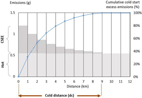
The new module implemented in QTraffic considers, as the first premise, that cold start emissions are an excess to hot running emissions and released during the cold distance, see Figure 1. The excess amount of emissions released under cold engines operation is distributed over the cold distance until the engine achieves normal operation temperature. Any trips shorter than the cold distance are expressed as a fraction of cold distance length.

Figure 1. A schematic representation of cold distance and cold start excess emissions – for a selected type of passenger cars at reference conditions (ambient temperature = 20 °C; average speed = 20 km/h) for CO. Cumulative CSEE during the trip are presented by blue line.

The methodology defined in André and Joumard (2005) was used to calculate cold distance (Equation (2)(2) $${dc}_{ik}=f(T,v,\mathrm{ }CC,\mathrm{ }\mathit{Fuel})$$(2) and Table 1). Thus, cold distance ($dc$) varies for each pollutant $i$ and technology $k$ according to: presence of catalytic converter ($CC$); fuel type (gasoline or diesel); ambient temperature ($T$) and vehicle speed ($v$). (2) $${dc}_{ik}=f(T,v,\mathrm{ }CC,\mathrm{ }\mathit{Fuel})$$(2)

Table 1. Parameters considered for cold distance ($dc$) estimation.

Period	Season	Ambient temperature
		Mean	Minimum	Maximum	Median
Morning period	Winter	8.7	1.6	16.5	8.2
	Spring	14.2	4.5	27.5	12.0
	Summer	18.2	12.5	28.7	17.5
	Autumn	13.1	4.5	20.2	14.0
Afternoon period	Winter	13.3	7.1	22.7	12.0
	Spring	18.5	7.7	33.7	17.5
	Summer	23.5	14.7	34.2	22.7
	Autumn	16.1	8.2	27.2	18.5

A two-step approach is implemented in CSEE module (Figure 3) starting from the quantification of emissions per trip for each Origin-Destination (O-D) pair (step 1), and then attribution of the emissions to the road segments (step 2), as described below.

Step 1 – Trip-based cold emissions:

Trip-based emissions are calculated considering O-D of trips and average speed for each road segment, provided by transportation model. For this purpose, VISUM traffic planning software (PTV-AG, 2013) was used considering: trip generation, trip distribution, modal split and traffic assignment. The traffic data obtained by modeling provides several advantages for the emissions quantification purpose in the comparison with real traffic point measurements due to their spatial coverage and possibility to preserve O-D information.

Assuming a possibility of different paths resulting from the traffic assignment, the trip-based CSEE for each O-D pair and pollutant $i$ ($\mathit{CSE}{E}_{ OD,i}$[g]) are calculated as following (Equation (3)(3) $$\mathit{CSE}{E}_{\mathrm{ }OD,i}=\sum _k\sum _{\mathit{path}}{w}_{i,k}\left(T,v\right)·h\left({\delta }_{\mathit{path},i,k}\right)·g_{i,k}\left(t\right)·N_{\mathit{path},k}\mathrm{ }\mathrm{ }$$(3) ): (3) $$\mathit{CSE}{E}_{\mathrm{ }OD,i}=\sum _k\sum _{\mathit{path}}{w}_{i,k}\left(T,v\right)·h\left({\delta }_{\mathit{path},i,k}\right)·g_{i,k}\left(t\right)·N_{\mathit{path},k}\mathrm{ }\mathrm{ }$$(3) where w – excess emissions [g.vehicle⁻¹] corrected for ambient temperature T [°C] and average vehicle speed v [km.h⁻¹]; h(δ_path,i,k = d_path/dc_i,k) is the dimensionless distance correction factor (defined in Equation (4)(4) $$h\left({\delta }_{i,k}\right)=\{\begin{array}{cc}\frac{1-e^{a_{i,k}·{\delta }_{i,k}}}{1-e^{a_{ik}}},& \delta \le 1\\ 1,& \delta >1\end{array}\mathrm{ }$$(4) ); $g(t)$ is the dimensionless correction factor for the parking time ($t$); and N is number of vehicles taking the same path.

For a given traveled distance d, a dimensionless correction factor h(δ) is defined with respect to the cold distance: (4) $$h\left({\delta }_{i,k}\right)=\{\begin{array}{cc}\frac{1-e^{a_{i,k}·{\delta }_{i,k}}}{1-e^{a_{ik}}},& \delta \le 1\\ 1,& \delta >1\end{array}\mathrm{ }$$(4) where δ = d/dc and a < 0 is a coefficient (tabulated values can be found in André & Joumard, 2005).

It is important to highlight that the emission factors from André and Joumard (2005) considered in this work are based on measurements only for passenger cars covering average speeds between 18.7 km/h to 41.5 km/h and ambient temperatures between −20 °C to 28 °C (André & Joumard, 2005). Therefore, the other types of vehicles, such as heavy-duty vehicles, are not considered in our study but it is expected that their contribution to cold start emissions will be limited in the urban context.

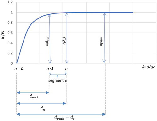
Step 2 – Cold emissions per road segment:

The CSEE calculated in the previous step are attributed to the road segments considering the path between an O-D pair, the road segments sequence and length. For this purpose, the road segments are defined regarding the intersections in the road network. For each segment n of the path ($d_{\mathit{path}}=\sum d_n$) the emissions are attributed in accordance with the Equation (5)(5) $${\mathit{CSEE}}_{\mathit{seg}\left(n\right),i}=\sum _k\left({\mathit{CSEE}}_{\mathit{path},i,k}·\frac{h\left({\delta }_{n,i,k}\right)}{h\left({\delta }_{\mathit{path},i,k}\right)}-{\mathit{CSEE}}_{\mathit{path},i,k}·\frac{h\left({\delta }_{n-1,i,k}\right)}{h\left({\delta }_{\mathit{path},i,k}\right)}\right)\mathrm{ }$$(5) and the distance correction factor h(δ) is presented in Figure 2. (5) $${\mathit{CSEE}}_{\mathit{seg}\left(n\right),i}=\sum _k\left({\mathit{CSEE}}_{\mathit{path},i,k}·\frac{h\left({\delta }_{n,i,k}\right)}{h\left({\delta }_{\mathit{path},i,k}\right)}-{\mathit{CSEE}}_{\mathit{path},i,k}·\frac{h\left({\delta }_{n-1,i,k}\right)}{h\left({\delta }_{\mathit{path},i,k}\right)}\right)\mathrm{ }$$(5)

Figure 2. The dimensionless correction factor h(δ) as a function of traveled and cold distances, where n represents a segment of the path.

Regarding the presented methodology, information on the O-D pair of each trip made within the study area is crucial to calculate trip-based cold start emissions and attribute them to the road network. For this purpose, data from VISUM are extracted (see Figure 3) considering: (i) road segments (segment ID, number of private cars, segment length, vehicle speed, etc.); (ii) paths (origin, destination, path ID, volume); and (iii) the road segments belonging to each path. These data are exported as .txt files and used as inputs for the CSEE module developed in Python Environment.

Figure 3. Conceptual framework of the CSEE module implemented in QTraffic.

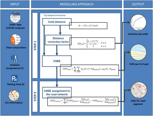
Figure 3 schematically presents the methodology developed in this study for cold start emission quantification at road segment level.

3. Case study

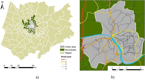
The CSEE module developed in this research was applied to the city of Coimbra to quantify cold emissions of carbon monoxide (CO), carbon dioxide (CO₂), oxides of nitrogen (NO_x) and hydrocarbon (HC) by considering 2019 as a reference year. Coimbra urban area (see Figure 4) is a part of a Municipality and a Region with the same name. According to PORDATA. (2021), the average population density for the Municipality and Region of Coimbra was around 441 hab.km⁻² and 101 hab.km⁻², respectively. It is third most important urban center of Portugal, after Lisbon and Porto, given its location and importance to the Centro Region and historical significance. Combining its strategic location and its attractiveness to study, work, health activities and leisure, important commuting movements take place in Coimbra urban area. Therefore, several travels have their origin or destination in this urban center, which is a crucial reason for quantifying the cold start emissions in this area. Although air quality has improved somewhat in recent years, some exceedances of the limit values defined by the European Air Quality legislation (Directive 2008/50/EC) have been recorded in the study area (Dias et al., 2016; Tchepel et al., 2020). Moreover, new Guidelines recently proposed by World Health Organization (2021) require more ambitious objectives for air pollution reduction. Being the road transport one of the most significant sources of air pollutants in the urban context (Agência Portuguesa do Ambiente, 2017), it is crucial to improve the quantification of the pollutant emissions and including the cold starts is crucial to guarantee the completeness of the emission estimates.

Figure 4. Traffic zones (a) and urban road network (b) considered in the study.

Regarding the previously described methodology, several input data are required (see Figure 3) to apply the CSEE module. The compilation of these inputs is described below.

3.1. Traffic data (VISUM outputs)

The information for each trip (number, average speed, origin and destination), requested for the CSEE step 1, were obtained from the VISUM traffic model applied for Coimbra. To characterize transport supply and demand in the study area, information from previous studies (Transport Innovation and Systems [TIS], 2011) was adapted considering: population and employment data by the zones; mobility indicators (travel generation rates, etc); private and public transport networks; transport costs per unit (fuel, parking and tariffs). According to Wardrop’s principle (Ortúzar & Willumsen, 2011), the traffic flow and average driving speed for each road segment of the transportation network was determined taking into account congestion effects. For the calibration and validation of the model the following information was used: travel distances; modal split; traffic for private transport and passenger counts of public transports; observations on trips duration.

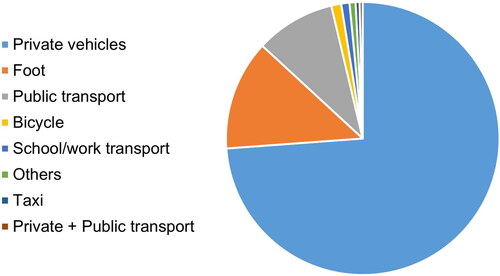
The scope of this study is to analyze cold start emissions within an urban area. However, the calculation of cold start emissions depends on the trip origin, which may be located outside of the study area. Therefore, the cold start emissions were obtained for a larger area. The Region selected (see Figure 4) has around 5835 km² and its transportation road network consists of 283 traffic generation zones (136 inside the urban center). About 18000 road segments were considered in this study with an average length of 130 m in urban area and about 600 m for the entire region. Traffic demand required for the transportation simulations was characterized based on daily O-D matrix considering different purposes, and transport modes (TIS, 2011). Figure 5 presents the modal share for passenger transport in the study Region considering active modes, private vehicles, public transport ant their combinations. Around 74% of the daily trips are made by private vehicles, which were selected for the application of the module. Based on previous studies (TIS, 2011), most of the daily trips occur in two periods: MP – morning period (from 8 AM to 10 AM; 25% of daily trips for the Region) and AP – afternoon period (from 4:30 PM to 7:30 PM; 30% of daily trips for the Region). Traffic counts recently performed within the study area confirmed these assumptions. The selection of both periods regards not only their representativeness in the traffic daily profile, but also the fact that cold emissions are higher with longer parking time. Although some travels occur in other periods of the day, they occur with a lower parking time and processed in the study as hot emissions only. We must highlight that in this study we only analyze working days.

Figure 5. Classification of daily trips by mode for the study Region. (Notes: “Private vehicles”: trips done by motorcycles or passenger cars; “School/work transport”: trips done by school or company vehicles (usually buses or minivans); “Others”: ambulances, tractors and others; “Private + Public transport”: trips done with a combination of private vehicles and public transport).

Figure 4b presents the urban road network by considering 5 road types, which will be crucial for the result analysis. The following hierarchical structure is considered for the road classification taking into account functional classes used in electronic navigable maps (NAVTEQ., 2011):

• Type 1 is attributed to roads that are allowed for high volume and maximum driving speed. These roads may have very rare or no speed variations.

• Road type 2 is used to direct traffic on road type 1 for travel between and through cities by the fastest way.

• Road type 3 links type 2 together and offers high traffic volumes with a lower level mobility than type 2.

• Type 4 connects with higher levels to collect and distribute road traffic between neighborhoods at a moderate speed.

• Type 5 all other roads, including pedestrian streets.

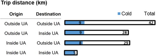
Due to importance of parking time, the cold start emissions were calculated separately for morning and afternoon periods. Hence, the daily cold start emissions are a result of a sum of both periods. It should be stressed that the number of starts at afternoon period within the urban area (UA) is significantly higher than at morning period due to trips “return to home.” The average trip distance and average cold distance are represented in Figure 6 for different clusters distinguishing O-D inside and outside the urbans area. Thus, the cold distance represents about 1/5 of the total trip with origin and destination outside the urban area, while for the trips that totally occurs inside the urban area it represents almost the total trip (around 96%).

Figure 6. Distance of total trip and under cold engine (blue bar), considering ambient temperature for winter season (explained below) and both afternoon and morning periods.

3.2. Ambient temperature

In order to calculate the cold distance for each pollutant and the cold start emission factors, seasonal variations of ambient temperature were analyzed (Table 2) using observations available for 2019 from the national meteorological station located in a proximity to the study area. To characterize the temperature for morning and afternoon periods for each season, median values were selected in order to reduce the impact of outliers.

Table 2. Local ambient temperature in 2019 considered for CSEE simulations.

Season	CO			CO2			HC			NOx
	1	2	3	1	2	3	1	2	3	1	2	3
Winter	1.62	17.93	0.33	688.95	7641.94	140.99	0.19	2.05	0.04	1.26	14.01	0.26
Spring	1.34	14.88	0.27	639.71	7095.75	130.91	0.15	1.63	0.03	1.26	13.98	0.26
Summer	1.05	11.66	0.22	583.34	6470.48	119.38	0.10	1.16	0.02	1.26	13.95	0.26
Autumn	1.27	14.10	0.26	624.72	6929.40	127.84	0.14	1.51	0.03	1.26	13.97	0.26

1 – Total daily emissions for the domain (t.day⁻¹).

2 – Daily emissions per inhabitant (g.day⁻¹.inhab⁻¹).

3 – Daily emissions per VKT (g.day⁻¹.VKT⁻¹).

3.3. Parking time

The parking time is required to calculate cold start emission factors. As a simplification, it was assumed that all starts at the morning period are initiated after the parking time equal or higher than 12 h, which means that the trips occur with a fully cooled engine (André & Joumard, 2005), while the parking time for the AP is influenced by working hours (in Portugal, 8 h working hours per day). Therefore, for cold emission the g(t) (i.e. is the correction factor for the parking time t) in Equation (2)(2) $${dc}_{ik}=f(T,v,\mathrm{ }CC,\mathrm{ }\mathit{Fuel})$$(2) will be 1 for the MP, while for AP it will take into account the 8 h parking time, resulting in correction factor g(t) less than 1 and thus lower emissions during the warm-up period.

3.4. Fleet composition

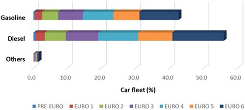
The information on vehicle technologies (i.e. Euro classes) and fuel properties is important to define the cold distance (see Equation (2)(2) $${dc}_{ik}=f(T,v,\mathrm{ }CC,\mathrm{ }\mathit{Fuel})$$(2) and Table 1) and the emission factors for each trip. The car fleet composition is presented in Figure 7. While the information on fuel properties was obtained based on statistical information for 2019 (Instituto Nacional de Estatística, 2020), the distribution by Euro classes was obtained from local measurements performed in selected crowded road of the studied transportation network (Martins, 2020).

Figure 7. Distribution of Coimbra’s passenger car fleet by fuel properties and Euro emission standards for 2019.

4. Results and discussion

Considering the research objectives, this section is divided in three subtopics. Firstly, a sensitivity analysis of the results provided by CSEE module is performed. Secondly, the daily exhaust emissions obtained for the case study are analyzed focusing on cold and hot contributions. Finally, the cold start emissions at road segments are evaluated.

4.1. Sensitivity analysis

In order to support the analysis of the results obtained in this study, the cold start emission factors are investigated and an example for Euro 4 gasoline and diesel passenger cars, that correspond to most of the modeled fleet, is presented. Figures 8–10 present the emissions as a function of the ambient temperature, parking time and average speed, respectively. This analysis is focused on the amount of pollutants emitted during the entire cold distance and the results are represented in terms of g/start (and not g/km).

Figure 8. Sensitivity of cold start excess emissions (g/start) to ambient temperature for Euro 4 gasoline and diesel passenger cars (average speed = 20 km/h; parking time = 12 h).

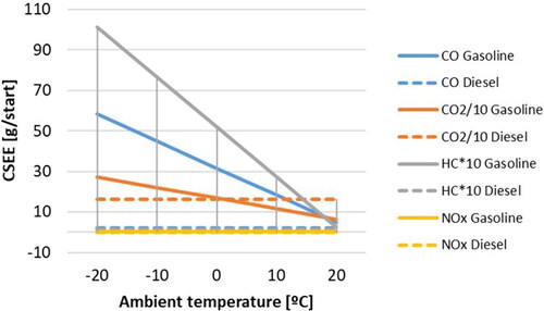
Figure 9. Sensitivity of cold start excess emissions (g/start) to parking time for Euro 4 gasoline and diesel passenger cars (average speed = 20 km/h; ambient temperature = 20 °C).

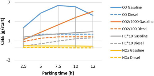
Figure 10. Sensitivity of cold start excess emissions (g/start) to average speed for Euro 4 gasoline and diesel passenger cars (parking time = 12 h; ambient temperature = 20 °C).

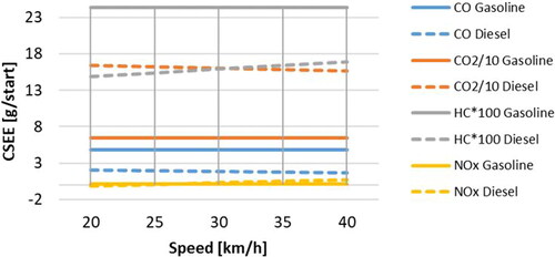
Compared to CO₂ and HC, CO emissions from gasoline cars grow steeply at lower temperatures, while NO_x emissions do not change. For diesel cars, the effect of ambient temperature is explicitly considered for technologies older than Euro 3 only (Table 1) and, therefore, the results presented in Figure 8 for diesel cars are affected by this assumption. With respect to parking time, the emissions of HC and CO₂ increase till 12 h of parking time, while CO emissions demonstrate non-linear behavior and NOx tend to decrease with the parking time. Although the average vehicle speed is very important for the cold distance calculation, the cumulative emissions along this distance expressed in g.start⁻¹ will be little affected by speed.

4.2. Contribution of cold starts to the daily exhaust emissions

The total daily emissions (in g/day) for Coimbra urban area are presented in Table 3 for different seasons. All the pollutants analyzed in this study (CO, CO₂, HC and NO_x) have significant contribution of cold start emissions as presented in Figure 11. As expected, the contribution of cold emissions for the NO_x daily emissions is much lower than for the other pollutants. For winter season the contribution of cold emissions to CO and HC is higher than 50%, because of the influence of ambient temperature (see Table 2 and Figure 11). It is important to highlight that these emissions are estimated using the median temperature for the winter season (8.2 °C for MP and 12 °C for AP), while the minimum observed is 1.6 °C and 7.1 °C (respectively) that will result in even higher emissions (around 9% to 25% increase, depending on the pollutant considered). Table 3 also presents the daily emissions per inhabitant and per vehicle kilometers traveled (VKT) in parenthesis, which may be relevant for comparison with other studies.

Figure 11. Contribution of cold and hot emissions to the total daily exhaust emissions in Coimbra urban area.

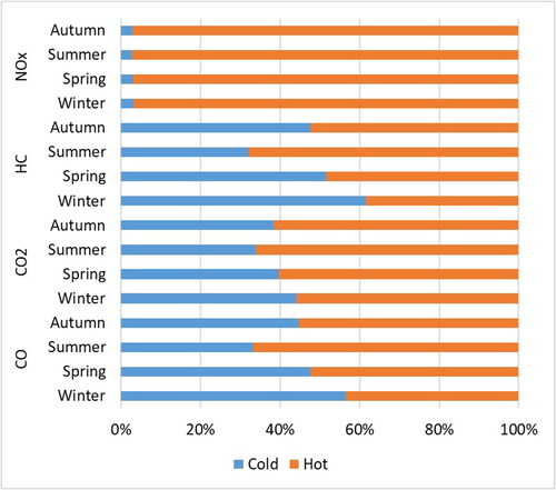
Table 3. Total daily emissions (hot + cold) in the Coimbra urban area considering different seasons.

Euro standard technologies	Diesel				Gasoline
	CO	CO2	HC	NOx	CO	CO2	HC	NOx
PRE-EURO	T, v	v	v	v	T, v	v	T, v	T, v
EURO 1	v	v	v	v	v	v	v	v
EURO 2	T, v	T, v	T, v	T, v	T, v	v	T, v	v
EURO 3	v	v	v	v	T, v	T, v	T, v	T, v
EURO 4-EURO 6	v	v	v	v	T	T	T	Constant

T – ambient temperature; v – vehicle speed.

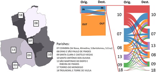
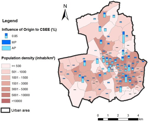
Figure 12 presents how the daily CSEE can be related to the origin and destination of a trip. First, it is important to stress that a large part of the trips under cold engine is related with trips that start or finish outside the urban area. In Figure 12 (right) only the CSEE that results from travels with O-D within the urban area are emphasized and aggregated by administrative units (parishes). Overall, the parishes that most generate trips and consequently emissions are also the most attractive parishes, except for parishes number 8 (“Eiras e São Paulo de Frades”) and number 13 (“São Martinho do Bispo e Ribeira de Frades”). This is because in the urban area, especial in the center of the city, residential areas may be located near working/studying areas. Therefore, the traffic induced CSEE at the beginning of a trip (residence or work), which will contribute to the local air pollution, will have its impacts in the population that are driving for their work (in the morning) or their residence (in the evening). However, is also important to point out, that the analysis at the parishes level may be too much aggregated to make these conclusions, therefore, further research must be done.

Figure 12. Distribution of daily cold start emissions, considering Origin and Destination of trips, for different administrative units in Coimbra urban area.

Information presented in Figure 13 highlights different contribution of cold emissions during the year. In all cases more than 50% of the CSEE occurs during the Morning Period due to lower ambient temperature and longer parking time. Furthermore, cold distance tends to decrease with the increase of ambient temperature (for instance for CO₂ it will reduce on average half a km from winter to summer). Therefore, due to lower ambient temperature during the morning period the cold distance will be higher, increasing the cold start emissions per vehicle during this period. AP and MP contributions will be different for different locations (Figure 14). Thus, AP contribution is very important in the locations with high proportion of commuting trips coming from outside the city. If during the morning period vehicles are entering to the urban area mainly with hot engine, the “return to home” trips are starting in the city and thus contribute to urban cold start excess emissions. Figure 14 presents the influence of a trip’s origin to the CSEE. One can see that for the AP most of the CSEE are related to the working/studying attraction poles, while for the MP the CSEE contribution is higher in residential areas (reinforcing the conclusions from Figure 12).

Figure 13. Contribution of each period (MP – Morning Period and AP – Afternoon Period) considered for the calculation of daily CSEE (in g/start).

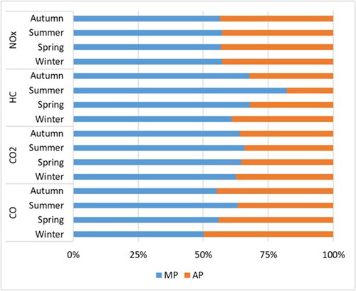
Figure 14. Influence of a trips’ origin to cold start excess emissions at Morning Period (MP) and Afternoon Period (AP).

4.3. Cold start excess contribution for line sources

In this subsection the CSEE at the road segment level for the worst situation (winter season) is analyzed. As an example, line sources are presented in Figure 15 showing CSEE contribution to the total daily emissions of CO. Overall, it is demonstrated that the greatest contributions occur on local roads (type 5). This finding is consistent with other research focused on cold start emissions at city level, such as Faria et al. (2018). Local roads mainly offer land access, providing the lowest mobility level.

Figure 15. (a) Contribution of cold sart CO emissions to the daily total (hot + cold) emissions for line sources (considering winter season); (b) and an example of the hot, cold and total emissions for a selected residential area in Coimbra.

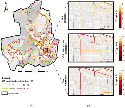
The frequency distribution of the data is depicted in Figure 16. A fraction of CSEE in the total (hot + cold) emissions is presented on vertical axis and the histogram analysis reveal how often different values occur on the road segments within the study area. It could be observed that for NOx the values are concentrated in a narrow range, mainly below 0.1 (i.e. CSEE contribution <10%). Also, the road segments classified as Type 1 reveal very low contribution of CSEE for all the pollutants that also confirmed by the statistics summarized in Table 4. However, it should be noted that only a small sample of the road segments classified as Type 1 is presented in the study domain, including a part of motorway close to the road entrance. Therefore, the results should not be extrapolated outside the urban area where, in general, no cold emissions could be expected for the Type 1. A left-skewed distribution is observed for other situations with an increasing importance of CSEE on the roads of Type 4 and Type 5. Thus, a significant number of values for CO and HC at local roads (Type 5) is above 0.9, i.e. CSEE contribution >90%. Also, local roads are characterized by higher variability in the comparison with other type of roads that confirmed by standard deviation and interquartile range presented in Table 4. Quantification of emissions with fine spatial resolution reveals inhomogeneities of CSEE contribution within the urban area and highlights a significant difference between the total values in urban inventory in a comparison with the results obtained for road segments. For example, cold start emissions contribute only 3% for daily NOx emissions at urban scale, but at individual road segment may achieve 43%. This contribution is different for the pollutants analyzed achieving 97%, 92% and 98% for CO, CO₂ and HC respectively. An example for CO is presented in Figure 15 showing inhomogeneities of cold start contribution at road segment level and the importance of emission quantification with fine spatial resolution. Thus, the example presented for a selected area (Figure 15b) reveal that cold emissions might duplicate or even quadruplicate in comparison to hot emissions.

Figure 16. Frequency distribution of CSEE contribution to daily emissions (hot + cold) for different type of roads during winter season.

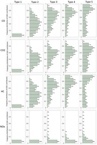
Table 4. Summary statistics of CSEE contribution (%) to daily emissions (hot + cold) for different type of roads considering winter season.

Pollutant	Type	Mean	Std Dev	75th Percentile	Median	25th Percentile
CO	1	0.7%	1.4%	1.2%	0.0%	0.0%
	2	39.3%	18.6%	53.8%	39.8%	23.9%
	3	57.3%	20.0%	73.3%	60.8%	45.3%
	4	63.8%	21.7%	79.3%	70.1%	51.6%
	5	60.8%	29.7%	87.4%	72.2%	33.3%
CO2	1	0.9%	1.5%	1.7%	0.1%	0.0%
	2	39.5%	14.4%	51.1%	38.4%	29.1%
	3	52.6%	16.1%	64.5%	55.4%	41.5%
	4	57.0%	16.9%	68.9%	59.7%	46.7%
	5	52.0%	25.1%	73.4%	58.6%	30.5%
HC	1	0.8%	1.6%	1.4%	0.0%	0.0%
	2	38.4%	19.9%	52.1%	37.4%	22.8%
	3	59.4%	20.9%	75.5%	63.5%	44.2%
	4	65.9%	23.0%	82.6%	72.8%	52.7%
	5	60.4%	32.0%	89.9%	72.1%	31.5%
NOx	1	0.1%	0.1%	0.1%	0.0%	0.0%
	2	3.9%	2.5%	5.6%	3.4%	1.9%
	3	5.9%	6.7%	7.5%	4.8%	2.8%
	4	6.0%	4.9%	7.6%	4.6%	2.7%
	5	8.0%	10.3%	12.5%	4.8%	1.2%

According to Reiter and Kockelman (2016), the cold start distance varies considerably from study to study. André and Joumard (2005) assessed a broad distribution (by pollutant) of cold start distance with an average of 5.2 km at 20 °C. In Figure 6, one may see that the parcel of a trip made with a cold engine will vary according to the region analyzed (outside the urban area: 21%; inside: 96%). Therefore, in densely developed cities a significant part of urban trips take place with a cold engine. The methodology applied in the current study demonstrates that the impact of cold starts increases from arterial to local streets. This founding is in agreement with previous studies (e.g. Faria et al., 2018) highlighting that higher emissions occur where most population live or work. Furthermore, from Figure 14 it is conclusive that most of the starts within the urban area that impact the daily emissions happen during the afternoon period (“return to home”), therefore, future mobility strategies should take this into consideration. With the analysis provided in this study it is possible to determine CSEE hotspots and trace their origin, which may play a key role in achieving the sustainable development goals regarding air quality and climate change issues. Therefore, future mobility and air quality policies should consider cold start impacts.

Thus, the advantages of different parking/transportation strategies could be evaluated considering additional benefits of the avoided emissions, in this case due to cold start emissions reduction. For example, environmental benefits of flexible-time communing or multimodal solutions, like Park&Ride, would be more evident if cold start emissions reduction could be considered additionally to hot emissions. However, such evaluation is only possible based on methodologies with fine spatial resolution and preserving O-D information to establish cause-effect relationships. Therefore, the modeling approach developed in this work could provide crucial input for the evaluation of environmental benefits and comparison of different transportation policies considering emissions reduction (hot + cold) at urban scale.

5. Conclusions

In this paper, a new modeling approach to quantify cold start emissions at road segment was proposed allowing spatial analysis of the cold start emissions for line sources. The CSEE module was developed and applied to the Coimbra urban area (Portugal). Both cold and hot emissions for line sources were calculated to obtain the total daily emissions and the cold start contribution.

The frequency distribution and summary statistics of the cold start contribution at a road segment level was analyzed for different types of roads. For winter season, a high contribution of cold start emissions is demonstrated with median values above 70% for CO and HC at road segments classified as type 5.

The total daily emissions (hot + cold) of CO, CO₂, HC and NOx for the urban area were analyzed considering their seasonal variations. For winter season the contribution of cold emissions for CO and HC is higher than 50%, but for NO_x is only 3%.

The cold start excess emissions during morning and afternoon periods were compared stressing the differences not only in absolute values but also in their spatial distribution. Thus, commuting trips of non-urban residents have no contribution to urban CSEE during the morning period if the trip is longer than “cold distance,” but their return trips originated near working/study locations in the city will be important for cold start emissions at afternoon period.

The modeling tool developed and applied in this study demonstrates the importance of quantifying cold start emissions with fine spatial resolution (i.e. at road segment level). There is large variability of CSEE contribution at urban roads that should not be neglected. Particularly, the data for local roads reveal higher variability that may contribute to the uncertainty of emission quantification in the locations where most people leave or work. These variabilities were possible to obtain because the model approach preserves the trip O-D pair information, being possible to attribute the cold emissions to each road segment of the path. Furthermore, the O-D information of a trip enables to access the contribution of different regions to the cold start emissions. In this context, the bottom-up modeling of cold start emissions and the preservation of O-D information would provide valuable information for traffic pollution studies and quantification of environmental benefits due to emissions (hot + cold) reduction.

Additional information

Funding

The research work was supported by PhD grant for Noela de Pina (PD/BD/128048/2016) funded by FCT – Fundação para a Ciência e Tecnologia.

References

- André, J. M., & Joumard, R. (2005). Modelling of cold start excess emissions for passenger cars (INRETS Report LTE 0509). Laboratoire Transports et Environment, INRETS.
- Agência Portuguesa do Ambiente. (2017). Agência Portuguesa do Ambiente – Emissões de Poluentes Atmosféricos por Concelho 2015: Gases acidificantes e eutrofizantes, precursores de ozono, partículas, metais pesados, poluentes orgânicos persistentes e gases com efeito de estufa. Anexo Emissões por concelho em 2015 (Excel format).
- Bishop, J. D., Stettler, M. E., Molden, N., & Boies, A. M. (2016). Engine maps of fuel use and emissions from transient driving cycles. Applied Energy, 183, 202–217. https://doi.org/10.1016/j.apenergy.2016.08.175
- Borge, R., de Miguel, I., de la Paz, D., Lumbreras, J., Pérez, J., & Rodríguez, E. (2012). Comparison of road traffic emission models in Madrid (Spain). Atmospheric Environment, 62, 461–471. https://doi.org/10.1016/j.atmosenv.2012.08.073
- Cifuentes, F., González, C. M., Trejos, E. M., López, L. D., Sandoval, F. J., Cuellar, O. A., Mangones, S. C., Rojas, N. Y., & Aristizábal, B. H. (2021). Comparison of top-down and bottom-up road transport emissions through high-resolution air quality modeling in a city of complex orography. Atmosphere, 12(11), 1372. https://doi.org/10.3390/atmos12111372
- Clairotte, M., Adam, T. W., Zardini, A. A., Manfredi, U., Martini, G., Krasenbrink, A., Vicet, A., Tournie, E., & Astorga, C. (2013). Effects of low temperature on the cold start gaseous emissions from light duty vehicles fuelled by ethanol-blended gasoline. Applied Energy, 102, 44–54. https://doi.org/10.1016/j.apenergy.2012.08.010
- Dardiotis, C., Martini, G., Marotta, A., & Manfredi, U. (2013). Low-temperature cold-start gaseous emissions of late technology. Applied Energy, 111, 468–478. https://doi.org/10.1016/j.apenergy.2013.04.093
- Dias, D., Tchepel, O., & Antunes, A. P. (2016). Integrated modelling approach for the evaluation of low emission zones. Journal of Environmental Management, 177, 253–263. http://dx.doi.org/10.1016/j.jenvman.2016.04.031
- Dias, D., Antunes, A. P., & Tchepel, O. (2019a). Modelling of emissions and energy use from biofuel fuelled vehicles at urban scale. Sustainability, 11(10), 2902. https://doi.org/10.3390/su11102902
- Dias, D., Pina, N., & Tchepel, O. (2019b). Characterization of traffic-related particulate matter at urban scale. International Journal of Transport Development and Integration, 3(2), 144–151. https://doi.org/10.2495/TDI-V3-N2-144-151
- Du, B., Zhang, L., Geng, Y., Zhang, Y., Xu, H., & Xiang, G. (2020). Testing and evaluation of cold-start emissions in a real driving emissions test. Transportation Research Part D: Transport and Environment, 86, 102447. https://doi.org/10.1016/j.trd.2020.102447
- European Environment Agency. (2011). The application of models under the European Union’s Air Quality Directive: A technical reference guide (Technical Report no. 10/2011).
- European Environment Agency. (2018). Progress of EU transport sector towards its environment and climate objectives (EEA Briefing No. 15/2018).
- European Environment Agency. (2019). Air quality in Europe — 2019 report (EEA Report No. 10/2019). https://doi.org/10.2800/822355
- European Monitoring and Evaluation Programme/European Environment Agency. (2019). Exhaust emissions from road transport. Passenger cars, light-duty trucks, heavy-duty vehicles including buses and motor cycles. European Monitoring and Evaluation Programme (EMEP) Air Pollutant Emission Inventory Guidebook 2019 (EEA Report No. 13/2019).
- Faria, M. V., Varella, R. A., Duarte, G. O., Farias, T. L., & Baptista, P. C. (2018). Engine cold start analysis using naturalistic driving data: City level impacts on local pollutants emissions and energy consumption. The Science of the Total Environment, 630, 544–559. https://doi.org/10.1016/j.scitotenv.2018.02.232
- Favez, J. Y., Weilenmann, M., & Stilli, J. (2009). Cold start extra emissions as a function of engine stop time: Evolution over the last 10 years. Atmospheric Environment, 43(5), 996–1007. https://doi.org/10.1016/j.atmosenv.2008.03.037
- FAIRMODE. (2010). Guidance on the use of models for the European Air Quality Directive. Forum for Air Quality Modelling in Europe – FAIRMODE (ETC/ACC Report Version 6.2).
- Fernandes, P., Bandeira, J. M., Fontes, T., Pereira, S. R., Schroeder, B. J., Rouphail, N. M., & Coelho, M. C. (2016). Traffic restriction policies in an urban avenue: A methodological overview for a trade-off analysis of traffic and emission impacts using microsimulation. International Journal of Sustainable Transportation, 10(3), 201–215. https://doi.org/10.1080/15568318.2014.885622
- Ferreira, E., Fernandes, P., Bahmankhah, B., & Coelho, M. C. (2022). Micro-analysis of a single vehicle driving volatility and impacts on emissions for intercity corridors. International Journal of Sustainable Transportation, 16(8), 681–705. https://doi.org/10.1080/15568318.2021.1919797
- Franco, V., Kousoulidou, M., Muntean, M., Ntziachristos, L., Hausberger, S., & Dilara, P. (2013). Road vehicle emission factors development: A review. Atmospheric Environment, 70, 84–97. https://doi.org/10.1016/j.atmosenv.2013.01.006
- Franco, V., Sánchez, F. P., German, J., & Mock, P. (2014). Real-world exhaust emissions from modern diesel cars: A meta-analysis of PEMS emissions data from EU (Euro 6) and US (Tier 2 Bin 5/ULEV II) diesel passenger cars – Part 1: aggregated results White paper. The International Council on Clean Transportation.
- He, L., Hu, J., Yang, L., Li, Z., Zheng, X., Xie, S., Zu, L., Chen, J., Li, Y., & Wu, Y. (2019). Real-world gaseous emissions of high-mileage taxi fleets in China. The Science of the Total Environment, 659, 267–274. https://doi.org/10.1016/j.scitotenv.2018.12.336
- Hood, C., MacKenzie, I., Stocker, J., Johnson, K., Carruthers, D., Vieno, M., & Doherty, R. (2018). Air quality simulations for London using a coupled regional-to-local modelling system. Atmospheric Chemistry and Physics, 18(15), 11221–11245. https://doi.org/10.5194/acp-18-11221-2018
- Instituto Nacional de Estatística. (2020). Estatísticas dos Transportes e Comunicações 2019.
- Jaworski, A., Kuszewski, H., Ustrzycki, A., Balawender, K., Lejda, K., & Woś, P. (2018). Analysis of the repeatability of the exhaust pollutants emission research results for cold and hot starts under controlled driving cycle conditions. Environmental Science and Pollution Research International, 25(18), 17862–17877. https://doi.org/10.1007/s11356-018-1983-5
- Laurikko, J. (1995). Ambient temperature effect on automotive exhaust emissions: FTP and ECE test cycle responses. Science of the Total Environment, 169(1–3), 195–204. https://doi.org/10.1016/0048-9697(95)04648-K
- Laurikko, J. (2008). Cold-start emissions and excess fuel consumption at low ambient temperatures-assessment of EU2, EU3 and EU4 passenger car performances [Paper presentation]. 16th International Transport and Air Pollution Congress. https://trid.trb.org/view/1084521
- Ludykar, D., Westerholm, R., & Almen, J. (1999). Cold start emissions at +22, -7 and -20 °C ambient temperatures from a three-way catalyst (TWC) car: Regulated and unregulated exhaust components. Science of the Total Environment, 235(1–3), 65–69. https://doi.org/10.1016/S0048-9697(99)00190-4
- Martins, M. G. (2020). Caracterização da matéria particulada em ambiente urbano [Dissertação de Mestrado Integrado em Engenharia do Ambiente, na área de Especialização em Território e Gestão do Ambiente]. Universidade de Coimbra.
- Mock, P., Tietge, U., Franco, V., German, J., Bandivadekar, A., Lambrecht, U., Ligterink, N., Lambrecht, U., Kühlwein, J., & Riemersma, I. (2014). From laboratory to road: A 2014 update of official and real-world fuel consumption and CO2 values for passenger cars in Europe White paper. The International Council on Clean Transportation.
- NAVTEQ. (2011). NAVTEQ’s NAVSTREETS street data reference manual v4.1. http://elodie.chaumet.free.fr/NAVSTREETS%20Reference%20Manual%20Q3%202011.pdf
- Ortúzar, J. D., & Willumsen, L. G. (2011). Modelling transport (4th ed.). Wiley.
- Outapa, P., Thepanondh, S., Kondo, A., & Pala-En, N. (2018). Development of air pollutant emission factors under real-world truck driving cycle. International Journal of Sustainable Transportation, 12(6), 432–440. https://doi.org/10.1080/15568318.2017.1384968
- PORDATA. (2021). Statistics about Portugal and Europa. Population density, according to census. https://www.pordata.pt/en/Municipalities/Population+density++according+to+the+Census-591
- PTV-AG. (2013). VISUM 13 user guide.
- Reiter, M. S., & Kockelman, K. M. (2016). The problem of cold starts: A closer look at mobile source emissions levels. Transportation Research Part D: Transport and Environment, 43, 123–132. https://doi.org/10.1016/j.trd.2015.12.012
- Tchepel, O., Dias, D., Ferreira, J., Tavares, R., Isabel Miranda, A., & Borrego, C. (2012). Emission modelling of hazardous air pollutants from road transport at urban scale. TRANSPORT, 27(3), 299–306. https://doi.org/10.3846/16484142.2012.720277
- Tchepel, O., Monteiro, A., Dias, D., Gama, C., Pina, N., Rodrigues, J. P., Ferreira, M., & Miranda, A. I. (2020). Urban aerosol assessment and forecast: Coimbra case study. Atmospheric Pollution Research, 11(7), 1155–1164. https://doi.org/10.1016/j.apr.2020.04.006
- Transport, Innovation and Systems. (2011). Modelo de planeamento de transportes dos sistemas de mobilidade do Mondego – Conceção e resultados (Report Volume 1).
- Varella, R. A., Duarte, G. O., Baptista, P., Villafuerte, P. M., & Sousa, L. (2017). Analysis of the influence of outdoor temperature in vehicle cold-start operation following EU real driving emission test procedure. SAE International Journal of Commercial Vehicles, 10(2), 596–697. https://doi.org/10.4271/2017-24-0140
- Weilenmann, M., Favez, J., & Alvarez, R. (2009). Cold-start emissions of modern passenger cars at different low ambient temperatures and their evolution over vehicle legislation categories. Atmospheric Environment, 43(15), 2419–2429. https://doi.org/10.1016/j.atmosenv.2009.02.005
- Weilenmann, M., Soltic, P., Saxer, C., Forss, A. M., & Heeb, N. (2005). Regulated and nonregulated diesel and gasoline cold start emissions at different temperatures. Atmospheric Environment, 39(13), 2433–2441. https://doi.org/10.1016/j.atmosenv.2004.03.081
- World Health Organization. (2021). WHO global air quality guidelines: Particulate matter (PM2.5 and PM10), ozone, nitrogen dioxide, sulfur dioxide and carbon monoxide. https://www.who.int/publications/i/item/9789240034228
- Zhang, Y., Lv, J., & Wang, W. (2013). Evaluation of vehicle acceleration models for emission estimation at an intersection. Transportation Research Part D: Transport and Environment, 18(1), 46–50. https://doi.org/10.1016/j.trd.2012.09.004
- Zheng, X., Lu, S., Yang, L., Yan, M., Xu, G., Wu, X., Fu, L., & Wu, Y. (2020). Real-world fuel consumption of light-duty passenger vehicles using on-board diagnostic (OBD) systems. Frontiers of Environmental Science and Engineering, 14(2), 1–10. https://doi.org/10.1007/s11783-019-1212-6