Siamese Convolutional Neural Networks to Quantify Crack Pattern Similarity in Masonry Facades

ABSTRACT

This paper proposes an automated approach to predict crack pattern similarities that correlate well with assessment by structural engineers. We use Siamese convolutional neural networks (SCNN) that take two crack pattern images as inputs and output scalar similarity measures. We focus on 2D masonry facades with and without openings. The image pairs are generated using a statistics-based approach and labelled by 28 structural engineering experts. When the data is randomly split into fit and test data, the SCNNs can achieve good performance on the test data ($R^2\approx 0.9$). When the SCNNs are tested on ”unseen” archetypes, their test $R^2$ values are on average 1% lower than the case where all archetypes are ”seen” during the training. These very good results indicate that SCNNs can generalise to unseen cases without compromising their performance. Although the analyses are restricted to the considered synthetic images, the results are promising and the approach is general.

KEYWORDS:

• Crack patterns
• deep neural network
• machine learning
• masonry structure
• regression
• similarity measure

1. Introduction

1.1. Motivation

Masonry buildings account for a large proportion of dwellings around the world. Assessing their conditions is mostly based on the detection of cracks as a primary sign of damage. In the Netherlands alone, every year house owners report hundreds of issues concerning cracks in masonry buildings. Addressing these problems requires identifying the most likely causes of the observed damage. While different damage causes can sometimes lead to comparable crack patterns (De Vent 2011a), similar causes often manifest through similar crack patterns. Quantification of crack pattern similarities is therefore instrumental to understand masonry damage.

Currently, the assessment of similarities between masonry crack patterns relies entirely on experts’ judgment. This implies several limitations:

• The quality of the evaluation strongly depends on the experience of the assessor, who needs to correlate the observed crack pattern with previously analysed and recorded ones.

• The assessment is affected by the expert’s understanding of global mechanisms and local conditions.

• Experts have difficulties in articulating and formalising their decisions, as it is not yet clear how the human brain performs the crack pattern comparison.

• The process is expensive, limited by the availability of experts, and provides only qualitative assessment.

This leads to a general lack of objectivity in crack analysis as different experts can provide substantially different interpretations for similar crack patterns.

Recent developments in machine learning may have the potential to overcome some of these limitations by providing tools for automated damage classifications. Significant effort has been devoted to crack detection from images, that is, the detection of cracks from photos without manual intervention, see e.g (Chaiyasarn et al. 2018; Hallee et al. 2021; Silva and Schwerz de Lucena 2018; Vu Dung and Le Duc 2019)., and semantic segmentation of cracks, see e.g (Dais et al. 2021; Garcia-Garcia et al. 2017). The latter is a classification technique that provides information on the location, length and width of cracks. Despite these important contributions, a consultation with structural masonry experts identified a lack of automated tools that could be applied to the practice of damage assessment at building scale. In particular, the structural masonry experts expressed their need for tools that could help them to identify plausible causes of the observed damage. To our knowledge, only a few authors have investigated this subject, see e.g. (Napolitano and Glisic 2019), hence damage identification in masonry building using advanced classification techniques remains a challenge.

1.2. Research objective

This paper is a step towards solving the above challenge by devising a model which can automatically quantify crack pattern similarities. We consider the development of such a model as an essential step in the development of instrumental and automated tools for damage assessment and damage cause attribution of masonry structures. In particular, the goal is to devise a function that takes two crack pattern images as inputs, and outputs scalar similarity measures that correlate well with assessment by structural engineers. The model can, for example, be used to compare an image from a cracked masonry building against a library of crack pattern images with known damage cause. Another potential application of the model is to use it in the calibration of a finite element model by maximising the predicted and observed crack pattern similarities where the design parameters of the calibration are parameters that characterise damage and/or damage source.

1.3. Approach

To quantify crack pattern similarity, we adopted Siamese convolutional neural networks (SCNNs), which are a particular class of deep neural networks. We used these flexible mathematical functions to take two images as input and to return a similarity score. To fit the model parameters of the neural network, we need data with at least a few hundreds of crack pattern images and corresponding similarities. Ideally, this data would come from real-world cases, but those are time consuming and expensive to collect. Moreover, the real-world cases can have multiple damage causes that are difficult to separate even by experts. Therefore, we used an alternative route to get the required data: a statistics-based approach using Markov walks was developed to generate synthetic crack patterns from 12 archetype classes. These archetype classes, which are sets of basic representative structures and damage patterns, contain (i) eight facades without openings but varying crack types, which we adopted from de Vent (De Vent 2011a); and (ii) four facades with openings, resembling typical existing dwellings in the Netherlands. Next, the generated crack pattern images were paired and then manually labelled by 28 structural engineers (raters) who judged their similarity on ordinal scales in three categories: crack pattern similarity, similarity in damage severity, and overall similarity. This was an important and time consuming part of the process, critical to guarantee a correct development and assessment of the model. For this reason, a separate evaluation of the labelling process was also performed. The labelled data was subsequently used to fit SCNNs with particular focus on testing their ability to generalise beyond the fitting data. For example, we evaluated the neural networks’ performance in predicting the similarity of image pairs which contain crack pattern archetypes classes that were not used for the fitting.

1.4. Scope

The labelled data that we used in this paper to fit a model for the quantification of the similarity between two crack patterns is based on synthetic crack patterns. Our assumption is that if the model fails to predict the crack pattern similarity using synthetic data, it will fail for real-world cases as well. If the model successfully predict the crack pattern similarity using synthetic data, it may be successful when applied to real-world cases as well, and future research can continue along that line.

1.5. Outline

Section 2 starts with a concise review of the literature on (crack pattern) similarity measures and the use of Siamese convolutional neural networks (SCNNs) in this context. Section 3 further describes the architecture of the SCNNs adopted in this paper. It also provides details on the performance metrics we used to assess the reliability of the annotated data and the predictive capabilities of the SCNNs. The three subsequent sections discuss the main steps of the approach to devise a model for an automated quantification of crack pattern similarities (Section 1.3): Section 4 explains how we generated the synthetic crack pattern images from the 12 archetype classes, Section 5 presents the labelling campaign to collect similarity scores of image pairs and an assessment of this labelled data, and Section 6 describes the fitting and testing of SCNNs on different data sets. The paper ends with a brief discussion of the results in Section 7 and the main conclusions in Section 8.

2. Literature review

In masonry structures, cracks can be the first warning of progressive damage (Cook et al. 2000). Crack pattern surveys provide valuable information on potential serviceability or stability issues (Binda, Cantini, and Tedeschi 2013; Valluzzi 2007). They typically involve classification of cracks based on their dimensions and geometry, and often include information on possible previous repairs and re-opening of retrofitted cracks (Saisi and Gentile 2020). Crack surveys are usually performed through expensive ground-level, tactile or drone-based inspections (Hallee et al. 2021), they depend on the competence of the visual assessor, and they are prone to human error (Akbari 2013; Phares et al. 2001). Due to these limitations, alternative approaches using automated image-based or visual damage assessment have been recently gaining popularity (Hallee et al. 2021).

One of the most important aspects of masonry damage assessment is to determine whether crack patterns are comparable and can be attributed to similar origins (de Vent, Rots, and van Hees 2013; Lourenço et al. 2014). Experts usually assess similarity based on their experience, comparing an observed pattern to a number of patterns they have seen before and remembered. In practice, this similarity is often determined qualitatively rather than quantitatively. To overcome this limitation, synthetically generated cracks, for example, from finite element models, have been used to attempt a quantitative estimation of crack similarities (Slobbe, Kraus, and Rozsas 2020). However, the sensitivity to the size and shape of the finite element mesh, and their inability to give unique solutions for a single damage cause, make these similarity measures unsuitable to assess crack patterns in an automated fashion (Slobbe, Kraus, and Rozsas 2020).

Shape similarity and open curve similarity metrics have also been developed for pattern recognition applications. However, most of these methods are not suitable for assessing crack pattern similarity, as they do not have a well-defined boundary or enclosed area that would allow them to match open curves (Chakmakov and Celakoska 2004). Partial matching of curves is also a challenge: when two shapes contain smaller similar portions, the dissimilarity must be smaller, and the measure should not excessively penalise regions that do not match (Veltkamp and Hagedoorn 2000). Finally, generic open curve similarity measures are not suitable for assessing crack pattern similarity as these measures define the shape as independent of the origin, location, and orientation of the curves under assessment. These parameters are critical in evaluating the severity and similarity of crack patterns and thereby identifying their damage cause. These measures also fail to account for the mechanical behaviour of brittle materials such as masonry.

Deep learning algorithms can be used to solve complex problems by generating appropriate mapping functions, provided that adequate labelled fitting data sets and acceptable models are available (Liu et al. 2017). A deep neural network is a computational model consisting of nodes that are organised into layers. Each node in a certain layer transmits a weighted signal to the other units in the next layer. A unit in the next layer sums these signals, applies a nonlinear function, and sends the result to the units in the next layer. Examples of tasks that are solved with deep neural networks are image classification, object detection, or language translation (Liu et al. 2017). The performance of the model on a task and data set is mathematically expressed in an objective function. Under a given data set, optimisation of this objective function with respect to the free parameters is called fitting of the model (or training in the machine learning community).

Especially convolutional neural networks (CNNs), that use convolutional filters, are suitable to automatically find patterns in images. Recent studies that use CNNs for automatic crack pattern assessment on images of such patterns are (Ali, Khan, and Chaiyasarn 2022; Bai et al. 2022; Dais et al. 2021; Loverdos and Sarhosis 2022; Rezaie et al. 2022; Silva and Schwerz de Lucena 2018; Wang et al. 2021). In a previous study, we developed neural network embeddings to calculate the similarity between different crack patterns of similar facades (Rozsas et al. 2020). Here, we demonstrated that a CNN can perform very well in classifying crack patterns belonging to different archetype classes (>99% accuracy), however, such a model cannot detect differences between patterns within a class. The results point to the need for reformulating the problem as a regression problem, that is, where one directly regresses the pairwise crack pattern similarity. For comparing two images, Siamese neural networks have shown to be suitable when ranking the similarity between inputs (Koch, Zemel, and Salakhutdinov 2015). A Siamese network embeds the inputs in the same space, after which a similarity score can be computed. We leveraged this method for assessing the similarity between two crack patterns.

3. Methods and tools

3.1. Siamese convolutional neural network

For the analysis of crack pattern similarity, we used a particular class of deep neural networks (Wang 2003): Siamese convolutional neural networks (Chicco 2021). In this work, we fitted the network to regress the similarity between crack pattern image pairs. The inputs of the network are crack pattern image pairs, and the outputs are three scalars, that is, three similarity measures.

To quantify the similarity of the crack patterns, we used Siamese convolutional neural networks. Convolutional neural networks (Arel, Rose, and Karnowski 2010) — a subclass of deep neural networks — take an image as their input and apply convolutional filters to this image. The parameters of the convolutional filters are also free model parameters. The filter sizes are hyperparameters and should be set by the user. The design of the Siamese convolutional neural network that was used in this work is shown in Figure 1, Its input layer consists of two raster images (pixels with colour information) and it has eight hidden layers made up of a combination of convolutional, max pool and dense layers. This model contains $\approx 2\cdot {10}^8$ free parameters.

Figure 1. Overview of the used Siamese convolutional neural network architecture. Conv: convolutional layer; maxpool: max pool layer; dense: fully connected layer; MSE: mean squared error.

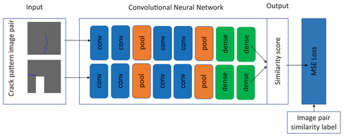
To minimise the selected mean squared error objective function we used the ADAM algorithm (Kingma and Ba 2017) and a StepLR scheduler,¹ that reduces the learning rate with a factor of 0.99 with each epoch. The initial learning rate was $1\cdot {10}^{-4}$ and the number of epochs was 40. Siamese neural networks are a type of network where two different inputs go through the same network and have a combined loss. In our case, after the crack pattern input has gone through the network, a similarity score is calculated. A mean square error loss is determined from the score computed by the network and the ground truth score of the image pair (Figure 1).

3.2. Performance metrics

This section describes the performance metrics used for assessing the agreement between raters (Section 3.2.1) and the predictive performance of the Siamese convolutional neural networks (Section 3.2.2).

3.2.1. Inter-rater reliability

The neural networks were fitted to assessments performed by structural engineers. The assessments focused on crack pattern similarity between image pairs (see the details in Section 5). To verify the level of consistency among the structural engineers, that is, the agreement of different experts on their assessment, a so-called inter-rater reliability index was calculated. Among the statistical measures for inter-rater reliability available in literature, we adopted Lin’s concordance correlation coefficient (I-Kuei Lin 1989) and (Krippendorff 2013).

Lin’s concordance correlation coefficient (CCC) measures the agreement between paired data (two raters). Where the Pearson correlation coefficient (Casella and Berger 2001) measures how closely two data sets are linearly dependent, irrespective of the straight line slope, Lin’s CCC is a metric that provides the correlation between two data sets on a straight line with a slope of 1.0 and passing through the origin. As the Pearson correlation coefficient, the value of Lin’s CCC can vary between −1 and 1. Lin’s CCC of −1 means perfect disagreement (i.e. discordance), 1 corresponds to perfect agreement (i.e. concordance), and 0 is no (Pearson) correlation between two data/measurement sets. When all data points are on the 45 degrees line there is perfect agreement. Opinions differ on how to interpret Lin’s CCC values other than −1 or 1. One way is to interpret it similarly to Pearson’s correlation, so, for example, a value $\le$ 0.2 indicates a poor agreement and a value $\ge$ 0.8 indicates a strong agreement (Altman, 1999). Another interpretation is given by (McBride 2005), where a value $\le$ 0.90 indicates poor agreement, a value between 0.90 and 0.95 moderate agreement, a value between 0.95 and 0.99 substantial agreement, and a value $\ge$ 0.99 excellent agreement. Irrespective of these interpretations, in the end it depends on the nature of the analysed case whether the agreement in the data is sufficient or not. In this paper, the threshold value for sufficient agreement was based on an analysis of the intra-rater agreement (i.e. the consistency of the raters with themselves) using Lin’s CCC value. More details are provided in Section 5.2.

The Krippendorff’s alpha measures the agreement between two or more raters. It can handle missing data, which is useful in our case because not all raters assessed the same or even the same number of image pairs. Krippendorff’s alpha varies between 0 and 1, where 0 indicates perfect disagreement (or unreliable data) and 1 indicates perfect agreement (or perfect reliability). (Krippendorff 2004) mentions that the acceptable level of agreement should depend on the consequences of drawing invalid conclusions from the data. When human lives are affected the criteria should be stricter than when “a content analysis is intended to merely support scholarly arguments”. For the latter, he suggested the alpha value to be at least 0.80, and preliminary conclusions can tolerate an alpha of 0.67 or larger.

3.2.2. Performance metrics for regression

To assess the performance of the fitted neural networks we used two metrics:

1. Coefficient of determination ($R^2$): a common measure for regression problems, it measures the proportion of total variation of outcomes explained by the model. Its domain ranges from $-\mathrm{\infty }$ to 1.0, a higher value indicating a better fit.

2. macro-averaged mean absolute deviation (MA-MAE): proposed by Baccianella et al. (Baccianella, Esuli, and Sebastiani 2009) for regression problems with ordinal categories (labels) and potentially imbalanced data sets. We selected this measure because in our labelling task we asked labellers to rate image pairs on an ordinal scale (as opposed to a continuous scale).

These metrics were computed for the fitting and testing data sets. For a good model, we expect the metrics computed on both data sets to be similar, for the $R^2$ metric to be as close as possible to one, and for the MA-MAE metric to be as close as possible to zero.

4. Generation of synthetic crack patterns

We propose a statistics-based simulation approach to generate synthetic crack patterns for a wide range of 2D masonry facades. This makes it possible to quickly (matter of seconds) generate a practically arbitrary number of crack patterns and in turn to test the potential of various crack pattern similarity measures.

The approach includes an algorithm that generates lines inside a predefined bounding box (i.e. the geometry of a facade) by means of Markov walks. The algorithm was generalised so that it can handle a parametric input of the facade and the cracks. This allows control over the dimensions of the facade, and the number, dimensions, and position(s) of the openings (doors and windows). It also enables control of the number of cracks, the crack initiation point(s), the crack angle(s), the crack length(s), the crack width over its length, and how jagged a crack is. Moreover, structural engineering considerations were imposed to increase the resemblance to reality. For example, in an iterative process dozens of generated crack patterns were shown to a masonry expert with decades of experience in structural damage assessment to get their feedback on what looks unrealistic and what would be a realistic alternative, then we adjusted our implementation accordingly, for example, through constraining certain parameters. Although the statistics-based simulation approach is not based on first physical principles, it is able to account for important crack pattern characteristics.

Section 4.1 explains the details of the crack pattern generation in masonry wall panels without openings and with a single crack. Section 4.2 presents a more realistic case, where crack patterns are generated in masonry facades that resemble typical existing dwellings in the Netherlands. These patterns are based on damage frequently observed in the field.

4.1. Masonry wall without opening

To support structural damage diagnosis in masonry structures, (De Vent 2011b) introduced 60 types of crack patterns (archetypes) along with their possible damage causes. From these, we selected eight without an opening (Figure 2). For consistency, the numerical IDs from (De Vent 2011b) were used here as well when referring to crack pattern archetypes. The eight archetypes share the following characteristics:

Figure 2. Illustrations of the selected eight crack pattern archetypes without openings. The images are adapted from (De Vent 2011b).

• a single wall panel is considered with a length over height ratio of 10 to 3;

• a single major crack characterises a pattern;

• no openings are present;

• a crack width linearly decreases to zero along the length of each crack.

Figure 3 shows the crack parametrization for a normalised (unit square) wall. Each crack was defined by the following parameters: the coordinates of the crack initiation point ($x_0,y_0$), the crack angle ($\alpha$), the crack length ($l_{\mathrm{c}\mathrm{r}\mathrm{a}\mathrm{c}\mathrm{k}}$), the maximum crack width (i.e. crack width at the initiation point) ($w_{\mathrm{c}\mathrm{r}\mathrm{a}\mathrm{c}\mathrm{k},0}$), and the jaggedness of the crack (${\sigma }_{\mathrm{c}\mathrm{r}\mathrm{a}\mathrm{c}\mathrm{k}}$). The first three parameters were randomly and uniformly sampled from an interval that is specified for each crack pattern archetype. The maximum crack width was randomly and uniformly sampled from an interval associated with one of the three considered crack width categories (Table 1). The crack width was linearly reduced to zero along the crack’s length.

Table 1. Considered maximum crack width categories.

Crack width category	Maximum crack width ($w_{\mathrm{c}\mathrm{r}\mathrm{a}\mathrm{c}\mathrm{k},0}$) interval [mm]
A	(Silva and Schwerz de Lucena 2018, de Vent, Rots, and van Hees 2013)
B	(de Vent, Rots, and van Hees 2013, Wang et al. 2021)
C	(Wang et al. 2021, Arel, Rose, and Karnowski 2010)

Figure 3. Illustration of the crack parametrization for facades without opening on a normalised (unit square) wall.

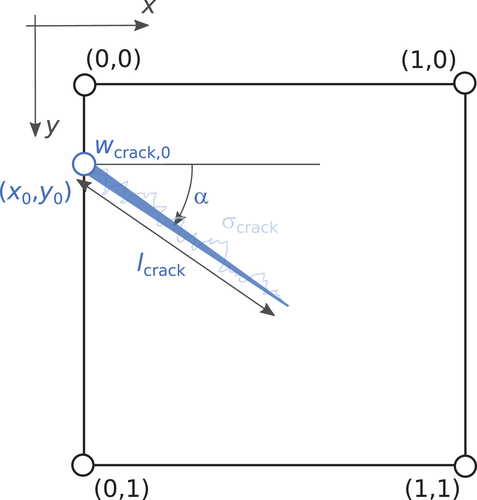
For illustration, the input values of these parameters for crack pattern archetypes 23, 30, and 31 are summarised in Table 2. In the simulation, the panel is discretised into disjoint rectangles and a crack can propagate only through the cells of this grid, one cell at a time/step. After a crack starts from the cell at ($x_0,y_0$), a random step is taken in either vertical or horizontal direction in a way that the expected global crack angle is $\alpha$. 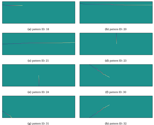The average absolute deviation from the expected direction is controlled by ${\sigma }_{\mathrm{c}\mathrm{r}\mathrm{a}\mathrm{c}\mathrm{k}}$, i.e. 0.5: highest deviation, 0: no deviation. Each crack is the widest at its initial point, from where the width is linearly reduced to zero along the crack’s length. Illustrative realisations of this simulation are presented in Figure 4, one for each crack pattern archetype with an opening. The simulated patterns illustrate that the proposed statistical approach can simulate realistic-looking and unique (due to the random component) crack patterns. The current implementation of the algorithm allows for the generation of a practically unlimited number of unique realisations of the eight selected crack pattern archetypes.

Table 2. Input values — in the unit square space — for crack pattern archetypes 23, 30, and 31. For the interpretation of the parameters see Figure 3.

pattern ID (p)	$x_0,y_0$*	$\alpha$ [deg]*	$l_{\mathrm{c}\mathrm{r}\mathrm{a}\mathrm{c}\mathrm{k}}$*	${\sigma }_{\mathrm{c}\mathrm{r}\mathrm{a}\mathrm{c}\mathrm{k}}$	$w_{\mathrm{c}\mathrm{r}\mathrm{a}\mathrm{c}\mathrm{k},0}$ [mm]*
23	[0.45, 0.55], [0, 0]	[87, 93]	[0.4, 0.6]	0.5	(de Vent, Rots, and van Hees 2013, Wang et al. 2021)
30	[0.05, 0.20], [0, 0]	(Liu et al. 2017, 70)	[0.3, 0.5]	0.5	(de Vent, Rots, and van Hees 2013, Wang et al. 2021)
31	[0, 0], [0.60, 0.80]	(Liu et al. 2017, 70)	2^†	0.5	(Silva and Schwerz de Lucena 2018, de Vent, Rots, and van Hees 2013)

* The lower and upper bounds of the uniform distribution.

^†To ensure that the crack goes through the entire wall.

Figure 4. One random crack pattern realisation for each crack pattern archetype (pattern ID) without openings. The colour along the cracks indicates the crack width: the darker, the wider the crack. See Figure 2 for the architectural representation of the matching crack patterns.

4.2. Masonry facades with openings

Every year in the Netherlands, house owners report hundreds of issues concerning cracks that appear in their masonry dwellings. In general, there are two main causes for these cracks: ($i$) uneven settlements; and ($ii$) constrained deformation due to temperature effects. The second cause mainly occurs in older masonry dwellings where dilatation joints are poor or even not present due to the heating of the roof or when the foundation constrains the facade.

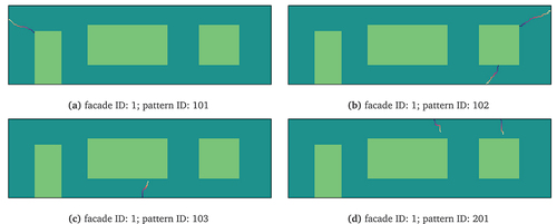
To simulate these cases we generated random crack patterns for 2D masonry facades of typical Dutch dwellings. Four different geometries were evaluated (Figure 5). One of them is detailed in Figure 6, showing one door opening and two window openings in the facade. Four crack pattern archetypes were considered, based on the following damage causes:

1. Cracking due to uneven settlement with a large settlement at the left side (pattern ID: 101).

2. Cracking due to uneven settlement with a large settlement at the right side (pattern ID: 102).

3. Cracking due to uneven settlement with large settlements at the middle (pattern ID: 103).

4. Cracking due to high temperature of the roof (pattern ID: 201).

Figure 5. Overview of the considered facades with openings. All facades have the same bounding rectangle dimensions (see Figure 6).

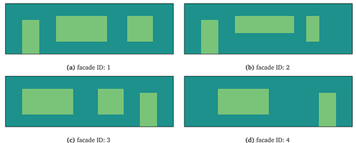
Figure 6. The dimensions (in meters) of the facade of a typical Dutch masonry dwelling (facade ID: 1).

Damage cause 1 and 3 typically lead to crack patterns with a single major crack, whereas damage cause 2 and 4 result in crack patterns with multiple cracks (we consider two cracks). As for the facades without openings, the crack widths were assumed to linearly decrease to zero along each crack length and to be the widest at their initiation point.

The crack patterns were created through the same approach used for the facades without openings. As an illustration, the parametrization of the two cracks in a facade subjected to damage cause 2 is shown in Figure 7. Individual cracks are identified by a numerical subscription, that is, 1 and 2 stand for the first and second crack respectively. Table 3 provides the input values of the crack parameters. The specified intervals of the crack initiation points are relative to the blue circles that are indicated in the corners of the right window. The specified intervals of the crack lengths are relative to the length of a fully developed crack (i.e. a crack that reached the edge of the facade or an opening). Figure 8 shows one illustrative realisation for each damage cause.

Table 3. Input values for crack pattern ID: 102. For the interpretation of the parameters see Figure 7.

$x_{0,1},y_{0,1}$ [cm]*	[−80, 0], [−20, 0] from the indicated corner in Figure 7
$x_{0,2},y_{0,2}$ [cm]*	[0, 80], [0, 0] from the indicated corner in Figure 7
${\alpha }_1$ [^°]*	[0, 70]
${\alpha }_2$ [^°]*	[225, 270]
$l_{\mathrm{c}\mathrm{r}\mathrm{a}\mathrm{c}\mathrm{k},1}$*	[0.4, 1.0] $\cdot l_{\mathrm{c}\mathrm{r}\mathrm{a}\mathrm{c}\mathrm{k};\mathrm{f}\mathrm{u}\mathrm{l}\mathrm{l}}$^†
$l_{\mathrm{c}\mathrm{r}\mathrm{a}\mathrm{c}\mathrm{k},2}$*	[0.4, 1.0] $\cdot l_{\mathrm{c}\mathrm{r}\mathrm{a}\mathrm{c}\mathrm{k};\mathrm{f}\mathrm{u}\mathrm{l}\mathrm{l}}$^†
${\sigma }_{\mathrm{c}\mathrm{r}\mathrm{a}\mathrm{c}\mathrm{k}}$	0.5
$w_{\mathrm{c}\mathrm{r}\mathrm{a}\mathrm{c}\mathrm{k},0,1}$ [mm]*	(de Vent, Rots, and van Hees 2013, Wang et al. 2021)
$w_{\mathrm{c}\mathrm{r}\mathrm{a}\mathrm{c}\mathrm{k},0,2}$ [mm]*	(Silva and Schwerz de Lucena 2018, de Vent, Rots, and van Hees 2013)

* The lower and upper bounds of the uniform distribution.

^†$l_{\mathrm{c}\mathrm{r}\mathrm{a}\mathrm{c}\mathrm{k},\mathrm{f}\mathrm{u}\mathrm{l}\mathrm{l}}$ is a fully developed crack to the edge of the facade.

Figure 7. Crack parametrization for the facade of a typical Dutch masonry dwelling (facade ID: 1) under damage cause 2 (pattern ID: 102).

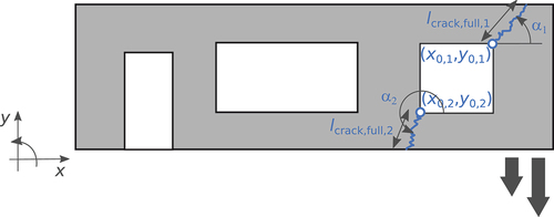
Figure 8. One random crack pattern realisation for each archetype (pattern ID) on a facade with openings. The colour along the cracks indicates the crack width: the darker, the wider the crack.

5. Labelling crack pattern pairs

5.1. Labelling campaign

Solving regression tasks require input and output pairs to which one fits models. The inputs (image pairs) are described in Section 4 and the corresponding outputs (similarity labels) are described in this section.

Twenty eight raters volunteered to assess the similarity of the crack pattern image pairs generated using the proposed statistics-based approach. Three similarity categories were used to perform the similarity assessment: crack pattern similarity, damage severity, and overall similarity. Each similarity category was rated using the following ordinal scale: very dissimilar, dissimilar, similar, very similar, and I cannot say. After the campaign, we noticed that the I cannot say label was only used for a few image pairs (0.7%) and the raters interpreted it inconsistently. Therefore, we excluded this label from the data used for the inter-rater analysis and neural network experiments. The remaining four labels were converted to numbers using the conversion table in Table 4. The three similarity categories were defined based on multiple discussions and a session with structural engineering experts:

• Crack pattern similarity label: The rater assesses the similarity of the crack patterns by considering the geometry of the crack (e.g. the crack initiation point and crack orientation) and the cracking mechanism.

• Damage severity label: The rater assesses the severity of the crack patterns by considering the crack length and the crack width.

• Overall similarity label: The rater assesses the overall similarity of the crack pattern image pair by combining the previous two labels, however they feel fit.

Table 4. Conversion table between textual and numerical labels.

Text label	Numerical label
Very dissimilar	0
Dissimilar	1
Similar	2
Very similar	3

Using the crack pattern ID and crack width category, we tried to have enough image pairs for each of the four labels (Table 4). This is only an approximation because at the time of the selection we did not yet have the labels. For example, to get potentially very similar patterns, 20% of the pairs were formed by images with the same pattern ID and crack with category per pair. Many similar labels were expected from image pairs that are formed by images with similar pattern ID (selected based on masonry domain knowledge) and same crack with category per pair. Table 5 summarises the selection criteria. About 45% of the image pairs have their pair formed by two images with the same pattern ID because (Rozsas et al. 2020) showed that the similarity assessment of these pairs is more difficult than pairs formed by two different pattern IDs. Following these criteria, 3000 image pairs were generated for the similarity assessment.

Table 5. Criteria to generate statistics-based crack pattern image pairs for labelling. For the crack width categories see Table 1.

Image pair selection criteria	Percentage of the sample [%]
Same pattern ID and same crack width category	20
Same pattern ID and any crack width category	25
Similar pattern ID and same crack width category	20
Similar pattern ID and any crack width category	25
Any pattern ID and any crack width category	10

We randomly and uniformly sampled values from the options defined by the rows.

The raters came from different academic backgrounds and had varying levels of experience working with masonry structures. A unique rater ID was assigned to each rater. Three broad expertise levels were defined: structural engineering experts, Ph.D. students, and M.Sc. students.

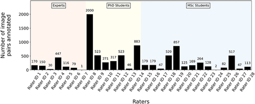
The labelling campaign was set up and performed using the Zooniverse.org platform. Of all the image pairs, only the ones assessed by at least three separate raters (before excluding the I cannot say label) were used to fit and test the neural network. Thus, a total of 2587 such image pairs were obtained. The number of labelled images by each rater and their level of expertise were summarised in Figure 9. For each similarity category, the labels given by the raters for a particular image pair were averaged to obtain a single scalar value, which is the required format for the used neural network. For additional details on the labelling campaign see Pillai (Ajithkumar Pillai 2022).

Figure 9. Summary of the number of image pairs labelled by each rater and their level of expertise (background).

5.2. Analysis of labels

We used Lin’s concordance correlation coefficient (CCC) and Krippendorff’s alpha to analyse the reliability of the data and the extent of agreement among the experts (see Section 3.2.1). In order to calculate Lin’s CCC the ordinal ratings very dissimilar, dissimilar, similar, and very similar were converted to integers from 0 to 3 respectively, as shown in Table 4. Although Krippendorff’s alpha can handle ordinal data, for consistency reasons we also used the data converted to integers for this inter-rater reliability measure.

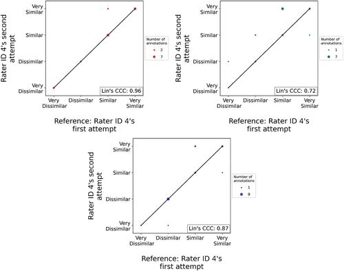
We considered two raters to be in sufficient agreement if their Lin’s CCC value was larger than the Lin’s CCC value belonging to the intra-rater agreement of a standard rater. Rater ID 4 was chosen as the standard rater due to their level of expertise and previous experience with assessing masonry structures. During the labelling task, Rater ID 4 annotated 23 image pairs twice, unaware that these image pairs were already annotated before. The data from these double-labelled image pairs were used to calculate the intra-rater agreement of the standard rater. Figure 10 agreement shows the consistency of the standard rater in the labelling of the same image pairs regarding the crack pattern similarity, damage severity, and overall similarity label. The corresponding Lin’s CCC values are 0.96, 0.72 and 0.87 respectively. It is interesting to observe the large differences between these values — particularly for the damage severity category — is far from perfect agreement. This indicates that even a trained masonry expert lacks full consistency in rating, probably due to the on-the-fly experience they gained during the labelling task. Based on these outcomes, we assumed that the Lin’s CCC value should be 0.70 or higher to show sufficient agreement with the standard rater in the assessment of the crack pattern similarity in masonry facades.

Figure 10. The intra-rater agreement of Rater ID 4 and the corresponding Lin’s CCC value for the crack pattern similarity label (a), the damage severity label (b), and the overall similarity label (c).

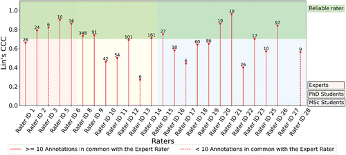
The raters who took part in this labelling task had varying academic backgrounds and degrees of experience regarding the assessment of masonry structures. In the following, we used Lin’s CCC to compare each rater with the standard rater (i.e. Rater ID 4). To compute Lin’s CCC value each rater and standard rater need to have assessed at least two image pairs in common. Preferably, to obtain a reliable value of Lin’s CCC, the number of assessed image pairs in common is 10 or larger (I-Kuei Lin 1989). The raters with IDs 7 and 24 did not have sufficient assessed image pairs in common with the standard rater, hence they were excluded from the analysis. From the remaining 26 raters, the raters with IDs 3, 13, 17, 27, and 28 had more than two but less than 10 assessed image pairs in common with the standard rater. While we still calculated their Lin’s CCC values, they should be considered with caution.

Figure 11 presents the Lin’s CCC value of each rater with respect to the standard rater for the crack pattern similarity label. Along the horizontal axis, the raters are grouped with respect to their expertise and background. The green shaded area at the top of the graph indicates Lin’s CCC values that reveal sufficient agreement (i.e. values of 0.70 or higher). The number above each rater’s CCC value represents the image pairs (or annotations) they have in common with the standard rater. It can be observed that 12 raters had sufficient agreement with the standard rater. Rater ID 3 belongs to this group but had less than 10 image pairs assessed in common. Rater ID 21 had the highest agreement with the standard rater, showing a Lin’s CCC value of 0.96. Rater ID 26 disagreed the most with the standard rater, showing a Lin’s CCC value of −0.25. As this value is too low, it was not plotted in Figure 11.

Figure 11. Lin’s CCC value of each rater with respect to the standard rater for the crack pattern similarity label. The number above each rater’s CCC value represents the image pairs (or annotations) they have in common with the standard rater.

Lin’s CCC value of each rater with respect to the standard rater were also calculated for the other two labels. Regarding the damage severity label, in general we observed much lower Lin’s CCC values, ranging from 0 (rater ID 27) to 0.71 (rater ID 10). Rater ID 21 alone showed sufficient agreement with the standard rater. Lin’s CCC values for the overall similarity label were in general slightly lower compared to the crack pattern similarity label with values between 0.11 (rater ID 13) and 0.88 (rater ID 21). Seven raters have sufficient agreement with the standard rater, though again Rater ID 3 has fewer than 10 assessed image pairs in common.

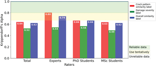
Krippendorff’s alpha was used to calculate the inter-rater reliability of each label for different groups of raters. Four groups of raters were considered: all 28 raters, and the raters that were denoted as Experts, PhD students, and MSc students in Section 5. The results are shown in Figure 12. All Krippendorff alpha values range between 0.49 and 0.80. Even using Krippendorff’s criteria for low-consequence content analysis (see Section 3.2.1), in general this metric reveals an unacceptable level of agreement among the raters, hence the data cannot be considered reliable. One exception is the subgroup Experts, where the Krippendorff alpha values of the crack pattern similarity label is 0.80, indicating sufficient agreement. The agreement for the overall similarity label of this group is also greater than 0.67, allowing us to draw preliminary conclusions.

Figure 12. Krippendorff’s alpha values of each label for four groups of raters.

In summary, the inter-rater reliability indices revealed a generally insufficient agreement between raters and the standard rater, and among groups of raters. In contrast, the within-group inter-rater reliability index of experts is sufficient. The low level of agreement may indicate that the questions in the labelling task were interpreted differently by the raters and/or by the limited experience of non-expert raters. This should be addressed in future studies, but for this work we deem the collected labels acceptable to fit neural networks to.

6. Analyses and results

6.1. Analysed cases

We analysed two sets of cases (Table 6):

• Interpolation: Based on a random split of the entire data set into fitting and testing sets. Identified by case IDs that start with letter ’A’.

• Extrapolation/generalizability: For each case, the testing set contains only image pairs where at least one of the pattern IDs is not present in any pair within the fitting data set. Identified by case IDs that start with letter ’G’.

Table 6. Overview of analysed cases. For the pattern IDs, the reader is referred to Figures 4 and 5.

Cases	Data for fitting		Data for testing
	Rater(s)	Pattern ID	Rater(s)	At least one from these pattern IDs	Possible pattern IDs to form a pair
A-A*	all raters	all	all raters	all	all
A-E*	only experts	all	only experts	all	all
A-S*	standard rater	all	standard rater	all	all
G-E-1	only experts	101, 103, 201	only experts	102	101, 102, 103, 201
G-E-2	only experts	all but 31	only experts	31	all
G-E-3	only experts	all but 18, 20, 21	only experts	18, 20, 21	all
G-E-4	only experts	all but 101	only experts	101	all
G-E-5	only experts	101,102,103, 201	only experts	all two digits IDs	all
G-E-6	only experts	23, 30, 32, 101, 103	only experts	24, 31, 102, 201	all
G-E-7	only experts	18, 20, 21, 30, 31, 32	only experts	23, 24	all two digits IDs
G-E-8	only experts	18, 20, 21, 23, 24, 30, 31, 32	only experts	all three digits IDs	all

*The fitting and testing sets are obtained by randomly splitting the data in a 3 to 1 ratio respectively.

For each case a neural network was fitted and tested with a particular combination of labelled data. The first three cases, ’A-A’, ’A-E’, and ’A-S’ use labelled image pairs from all the pattern IDs in facades without and with openings. They differ with respect to the data labellers: ’A’, all raters, `E`, only the experts (see Section 5.1), and `S`, only the standard rater (i.e. Rater ID 4, see Section 5.2). We randomly split the data into subsets for fitting (75%) and for testing (25%) for these three cases. The cases ’G-E-1’ to ’G-E-8’ leave out one or multiple pattern ID(s) from the fitting and evaluate how well the neural network can predict the similarity of these unseen crack pattern image pairs. In these eight cases only labelled image pairs from the experts were used, since this group showed the highest within group agreement. For each ’G’ case the fitting and testing image pairs are formed by all images that fulfil the criteria listed in the corresponding row of Table 6. This also means that when these analyses are repeated the variability in the outcomes solely comes from the pseudo-randomness of the optimisation algorithm used for fitting the neural network.

The ’G’ cases were selected to test various extents of generalizability ranging from “easy” ones, where only one pattern ID is excluded from the fitting (e.g. ’G-E-2’), to “hard” ones, where we test the generalisation to other facade geometries and crack patterns (e.g. ’G-E-5’).

6.2. Results

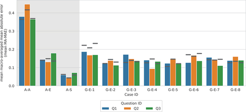
The performance measures $R^2$ and MA-MEA — calculated for the fit and test data set for each case — are summarised in Figures 13 and 14, respectively. The plots show the computed mean values of $R^2$ and MA-MEA from five analyses with different random seeds. Both performance measures revealed a comparable pattern across all cases and for all three questions; therefore, when discussing the results we focus on the easier to interpret $R^2$ measure. Irrespective of the case, the highest predictive performance was achieved for Q1, in most cases closely followed by Q3 (on average 2% lower $R^2$ values), and tailed by Q2 on average by a 9% lower $R^2$ value.

Figure 13. Mean $R^2$ performance measures for testing data (bars) and fitting data (horizontal lines). White background highlights the generalizability (G) cases.

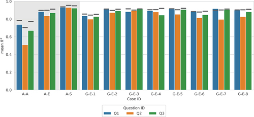
Figure 14. Mean macro-averaged MAE performance measures for testing data (bars) and fitting data (horizontal lines). White background highlights the generalizability (G) cases.

In general, the mean $R^2$ values for the fit and test data are reasonably close, showing slightly lower values for the latter. Exceptions to this were found for Q2 where the differences are significantly larger, and for Q1 in a few ’G’ cases where the mean $R^2$ values for the test data are slightly higher than for the fit data. The mean MA-MEA values show a similar overall pattern.

Out of the interpolation (’A’) cases the one with only the standard rater performs the best with mean $R^2$ values between 0.92 and 0.93, closely followed by the expert raters with mean $R^2$ values between 0.88 and 0.91, and tailed with a considerable gap by all raters with mean $R^2$ values between 0.51 and 0.74. This ranking is expected considering the consistency in the data (i.e. the agreement among the raters) used for fitting the neural network. For instance, a considerably larger inconsistency was observed for the total group of raters compared to the group with only experts (see Figure 12). The more inconsistency in the data, the more difficult it is to fit a neural network that can make accurate predictions.

For the extrapolation or generalizability (’G’) cases mean $R^2$ values between 0.80 and 0.92 were observed. The corresponding models show comparable performance to the model from the interpolation case ’A-E’ that has the same labellers. This striking outcome indicates that the neural networks can generalise to unseen crack types (archetypes) — often to substantially different ones — without compromising their performance. Case ’G-E-5’ and ’G-E-8’ are particularly interesting. The fit data for case ’G-E-5’ solely consisted of image pairs of facades with openings, while 93% of the image pairs in the test data were pairs where both members have an image of a facade without openings (Figure 16). And for case ’G-E-8’: the fit data solely consisted of image pairs of facades without openings, while 86% of the image pairs in the test data were pairs where both members have an image of a facade with openings (Figure 17). So, these two neural networks were predominantly tested on labelled data with different facade geometries than used for fitting and still are able to make predictions close to and sometimes even outperforming the ’A-E’ interpolation case that we used as a reference.

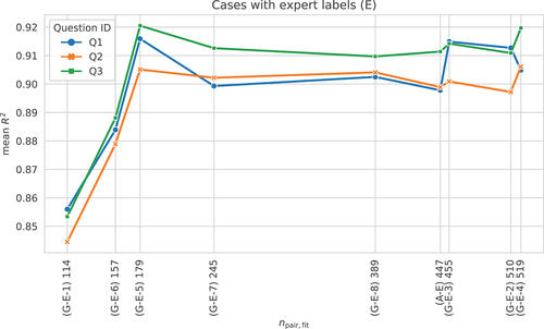
The worst generalizability performance was obtained for the ’G-E-1’ case that used only facades with openings and meant to test the generalizability from three archetypes to a fourth “unseen” one. In light of the other results, this relatively poor performance is likely attributable to the small number of pairs used for the fitting, only 114, which is less than one-fourth of the average number of pairs used for fitting across all cases (Figure 15).

Figure 15. Mean $R^2$ as a function of the number of pairs used for the fitting ($n_{\mathrm{p}\mathrm{a}\mathrm{i}\mathrm{r},\mathrm{f}\mathrm{i}\mathrm{t}}$).

Additional results are presented in Annex A, for example, the standard deviation of the performance metrics across a few runs and the number of image pairs used for fitting and testing are shown in Table 7. Most standard deviations are negligibly small, for example, <0.03 for the $R^2$ metric.

7. Discussion

Except for case ’A-A’, the neural networks result in relatively high $R^2$ and low MA-MEA values for both interpolation and extrapolation tasks. These good outcomes are promising and encourage the exploration of more complex cases with realistic data. Nevertheless, there are some aspects that are important to consider for the interpretation of the results. First, it is yet unknown what accuracy is required to use this crack pattern similarity measure, for example, for the calibration of finite element models. Second, we noticed that for all cases some combinations of possible pair IDs (archetypes) are over-represented (by design) in the fit and test data, while others are rarely, or even not at all, labelled (Figures 16 and 17). It is not clear whether the relatively high $R^2$ scores would also be obtained if the data sets contained more evenly distributed combinations of pair IDs. Note that in general the data is sufficiently balanced with respect to the different ratings. Figure 15 indicates that for some cases the fitting data set is too small and should be increased to above 200 in future studies.

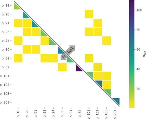
Figure 16. Case ’G-E-5’: number of image pairs ($n_{\mathrm{p}\mathrm{a}\mathrm{i}\mathrm{r}}$) per unique crack pattern ID pairs (for brevity a crack pattern ID is indicated by ’p’ followed by an ID number). Cells without colour correspond to pairs that are not present in the data set.

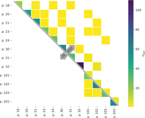
Figure 17. Case ’G-E-8’: number of image pairs ($n_{\mathrm{p}\mathrm{a}\mathrm{i}\mathrm{r}}$) per unique crack pattern ID pairs (for brevity a crack pattern ID is indicated by ’p’ followed by an ID number). Cells without colour correspond to pairs that are not present in the data set.

To get some insight into the prediction performance of the fitted model, a few illustrative pairs with poor and good predictions are shown in Figure 18. By visually inspecting a number of image pairs and predictions, we observed that poor performance typically occurs for cases where the labellers disagreed. It is a limitation of the model formulation that the model cannot “learn” this disagreement.

Figure 18. Poor and good model prediction examples from case A-A and question Q3.

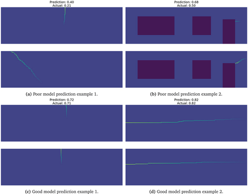
Figure 19. Mean MA-MAE as a function of the number of pairs used for the fitting ($n_{\mathrm{p}\mathrm{a}\mathrm{i}\mathrm{r},\mathrm{f}\mathrm{i}\mathrm{t}}$).

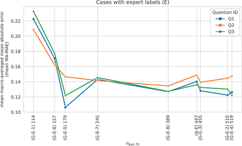
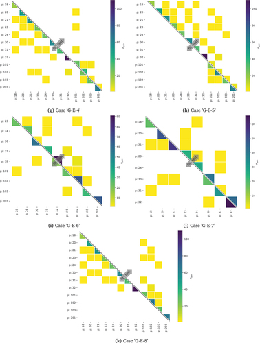
Figure 20. All cases: number of image pairs ($n_{\mathrm{p}\mathrm{a}\mathrm{i}\mathrm{r}}$) per unique crack pattern ID pairs (for brevity a crack pattern ID is indicated by ’p’ followed by an ID number). Cells without colour correspond to pairs that are not present in the data set. Some plots that appear in the main body of the article are repeated here for convenience (continued on the next page).

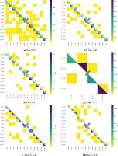
Figure 20. (continued).

By averaging the answers of the labellers given for the same pairs, we throw away valuable information. This means that some variability in the labels is already lost before starting to fit the neural networks. The averaging is done because of the chosen modelling approach but there are different model formulations that could use all collected data, e.g. Bayesian neural networks (Lampinen and Vehtari 2001; Mackay 1995).

Moreover, neural networks are known to have sensitive input-output mappings. Despite their high prediction accuracy, their performance can drop significantly upon small modifications of the images (Szegedy et al. 2014), indicating that they did not “learn” the characteristic and defining features. This should make us cautious in our expectations of neural network predictions on crack pattern similarities even for other synthetic crack patterns, let alone for real world ones.

An important limitation of this work is that it deals solely with synthetic data that are inspired by observed crack patterns of residential buildings in the Netherlands. The extrapolation of the fitted SCNNs were tested only within this scope. We expect that an accurate extrapolation to other construction practices would be much harder, if feasible at all.

The presented approach can be extended to real-world data. It would require collecting and processing crack-pattern images, at first of similar structures. After manual labelling the image pairs, SCNNs could be fitted to the data and their performance could be evaluated using the same methodology used in this paper. The value of the fitted SCNNs should be assessed based on their intended application, which will require further specific studies.

8. Conclusions

This paper aims to contribute to the automation of the condition assessment for masonry structures. We focused on devising a function that takes two crack pattern images as inputs and outputs scalar similarity measures that correlate well with assessment by structural engineers. We used Siamese convolutional neural networks to regress the similarities between synthetic crack pattern image pairs. We proposed a statistics-based approach to generate synthetic crack pattern images while taking account of characteristic features like crack location, orientation, length, and width. The similarities between the generated image pairs were assessed by 28 structural engineers. The agreement between experts was evaluated through inter-rater reliability analyses. These revealed insufficient agreement between all raters and an acceptable agreement between experts. Siamese neural networks were fitted to the obtained image pair–similarity labels pairs. Eleven cases were formed by splitting the data into fitting and testing data. These either test the interpolation or the extrapolation (generalisation) ability of the neural networks.

We found that the expertise of the raters who provided the input data has a big influence on the performance of the neural networks. In the interpolation case, where data from all raters are used, the obtained $R^2$ values for the test data range between 0.74 and 0.51. When only data from the expert raters are used, these numbers increase to 0.88 and 0.91 respectively, which is a substantial improvement. Based on these results, we only used the data from expert raters for the extrapolation cases.

The extrapolation cases were selected to test various extents of generalizability ranging from “easy” ones, where only one pattern ID was excluded from the fitting (e.g. ’G-E-2’), to “hard” ones, where we tested the generalisation to other facade geometries and crack patterns (e.g. ’G-E-5’). For all cases, the neural networks’ performance is excellent (Figure 13). Their test $R^2$ values are very close (on average less than 1% difference) to what is obtained for the interpolation case with expert data, which we consider as a reference. These excellent results indicate that the neural networks can generalise to unseen crack pattern types — often to substantially different ones — without compromising their performance. A striking case is ’G-E-8’ where the fitting data solely consists of image pairs of facades without openings while 86% of test image pairs are formed by only images of facades with openings, often with a crack cause that is not present in the fitting data.

As a next step, it should be understood why and how this excellent generalisation happens and how robust it is to changes in the inputs and/or outputs. Moreover, it needs to be analysed what prediction accuracy is sufficient and desirable to support the condition assessment of masonry structures. It should be reiterated that all presented results are based on synthetic crack patterns generated using a particular statistics-based approach, for example, individual cracks are a single pixel wide and only the major cracks are present. The scope is further restricted by that the synthetic crack pattern generation is inspired by observed crack patterns of residential buildings in the Netherlands. Despite the limitations, the results are promising and the approach is general.

Author contributions

A.R., A.S., and W.H. conceived the study. A.S., G.G, K.A.P., and A.R. designed the labelling campaign and participated in the labelling (among other volunteers). K.A.P. and K.K. set up and managed the labelling campaign in Zooniverse.org. K.A.P. performed the analyses of the collected similarity labels including the inter-rater reliability analyses. A.R., A.S. and G.G. acted as supervisors. A.R. implemented the code for generating the statistics-based crack patterns with contribution from K.K. W.H. implemented the code of the Siamese convolutional neural network and performed the related analyses with the assistance of M.K. A.R. and K.A.P. prepared the figures. A.R., A.S., and G.G. drafted the majority of the paper relying on the thesis of K.A.P. All authors contributed to the writing of the paper and commented on the manuscript at all stages.

Data availability

The data that support the findings of this study are available from the authors upon request.

Software availability

The code that supports the findings of this study is available from the authors upon request.

Acknowledgments

We are grateful to Huibert Borsje (TNO) for valuable discussions on damaged masonry structures. We are indebted to all the labellers who volunteered their time and expertise to label image pairs. This publication uses data generated via the Zooniverse.org platform, development of which is funded by generous support, including a Global Impact Award from Google, and by a grant from the Alfred P. Sloan Foundation.

Disclosure statement

No potential conflict of interest was reported by the author(s).

Notes

¹ https://pytorch.org/docs/stable/generated/torch.optim.lr_scheduler.StepLR.html.

A Regression results

This annex provides additional details of the regression results (Figures 19 and 20). Each standard deviation (std) in Table 7 is computed from the results of five times fitting the neural network using the same data for fitting across all the fittings (same applies to the testing data). This means that the standard deviation only measures the variability due to the pseudo-randomness of the optimisation algorithm used for fitting the neural networks.

Table 7. Summary of the regression performance measures for all considered cases.

Case ID	Question ID	Data set	mean $R^2$	std $R^2$	mean MA-MAE	std MA-MAE	$n_{\mathrm{p}\mathrm{a}\mathrm{i}\mathrm{r}}$
A-A	Q1	test	0.7382	0.0132	0.3799	0.0099	647
A-A	Q1	fit	0.7828	0.0180	0.3650	0.0136	1940
A-A	Q2	test	0.5088	0.0310	0.4476	0.0142	647
A-A	Q2	fit	0.7041	0.0298	0.4167	0.0296	1940
A-A	Q3	test	0.6698	0.0293	0.3653	0.0175	647
A-A	Q3	fit	0.7721	0.0168	0.3690	0.0201	1940
A-E	Q1	test	0.8841	0.0163	0.1450	0.0252	150
A-E	Q1	fit	0.8978	0.0148	0.1402	0.0240	447
A-E	Q2	test	0.8370	0.0120	0.1313	0.0101	150
A-E	Q2	fit	0.8989	0.0089	0.1488	0.0167	447
A-E	Q3	test	0.8702	0.0151	0.1792	0.0267	150
A-E	Q3	fit	0.9114	0.0117	0.1360	0.0200	447
A-S	Q1	test	0.9322	0.0105	0.0593	0.0229	112
A-S	Q1	fit	0.9372	0.0148	0.0625	0.0153	336
A-S	Q2	test	0.9310	0.0041	0.0456	0.0169	112
A-S	Q2	fit	0.9537	0.0094	0.0437	0.0127	336
A-S	Q3	test	0.9227	0.0099	0.0723	0.0034	112
A-S	Q3	fit	0.9494	0.0091	0.0592	0.0139	336
G-E-1	Q1	test	0.8357	0.0155	0.1871	0.0343	65
G-E-1	Q1	fit	0.8560	0.0155	0.2224	0.0217	114
G-E-1	Q2	test	0.7980	0.0396	0.1683	0.0376	65
G-E-1	Q2	fit	0.8445	0.0541	0.2084	0.0505	114
G-E-1	Q3	test	0.8282	0.0089	0.1701	0.0281	65
G-E-1	Q3	fit	0.8534	0.0134	0.2326	0.0206	114
G-E-2	Q1	test	0.9153	0.0079	0.1214	0.0209	87
G-E-2	Q1	fit	0.9127	0.0114	0.1225	0.0149	510
G-E-2	Q2	test	0.8730	0.0224	0.1387	0.0206	87
G-E-2	Q2	fit	0.8972	0.0035	0.1447	0.0092	510
G-E-2	Q3	test	0.8920	0.0187	0.1127	0.0148	87
G-E-2	Q3	fit	0.9109	0.0123	0.1303	0.0130	510
G-E-3	Q1	test	0.8827	0.0137	0.1719	0.0293	142
G-E-3	Q1	fit	0.9149	0.0117	0.1281	0.0171	455
G-E-3	Q2	test	0.8933	0.0061	0.1480	0.0208	142
G-E-3	Q2	fit	0.9009	0.0191	0.1393	0.0315	455
G-E-3	Q3	test	0.9198	0.0129	0.1377	0.0292	142
G-E-3	Q3	fit	0.9142	0.0076	0.1325	0.0166	455
G-E-4	Q1	test	0.8945	0.0183	0.1410	0.0227	78
G-E-4	Q1	fit	0.9049	0.0178	0.1262	0.0205	519
G-E-4	Q2	test	0.8798	0.0115	0.0939	0.0130	78
G-E-4	Q2	fit	0.9061	0.0158	0.1473	0.0275	519
G-E-4	Q3	test	0.8444	0.0333	0.1335	0.0193	78
G-E-4	Q3	fit	0.9197	0.0092	0.1224	0.0111	519
G-E-5	Q1	test	0.9162	0.0121	0.1232	0.0133	418
G-E-5	Q1	fit	0.9159	0.0189	0.1063	0.0232	179
G-E-5	Q2	test	0.8535	0.0078	0.1476	0.0105	418
G-E-5	Q2	fit	0.9051	0.0114	0.1465	0.0222	179
G-E-5	Q3	test	0.9070	0.0101	0.1228	0.0174	418
G-E-5	Q3	fit	0.9205	0.0085	0.1218	0.0217	179
G-E-6	Q1	test	0.8869	0.0197	0.1271	0.0172	298
G-E-6	Q1	fit	0.8839	0.0156	0.1707	0.0274	157
G-E-6	Q2	test	0.8138	0.0100	0.1669	0.0164	298
G-E-6	Q2	fit	0.8789	0.0185	0.1622	0.0385	157
G-E-6	Q3	test	0.8484	0.0093	0.1367	0.0158	298
G-E-6	Q3	fit	0.8881	0.0139	0.1773	0.0322	157
G-E-7	Q1	test	0.9168	0.0122	0.1559	0.0336	144
G-E-7	Q1	fit	0.8993	0.0153	0.1431	0.0218	245
G-E-7	Q2	test	0.7957	0.0198	0.1435	0.0279	144
G-E-7	Q2	fit	0.9022	0.0093	0.1416	0.0093	245
G-E-7	Q3	test	0.9076	0.0092	0.1106	0.0091	144
G-E-7	Q3	fit	0.9126	0.0146	0.1455	0.0166	245
G-E-8	Q1	test	0.8994	0.0112	0.1385	0.0141	208
G-E-8	Q1	fit	0.9025	0.0181	0.1270	0.0236	389
G-E-8	Q2	test	0.8276	0.0102	0.1603	0.0240	208
G-E-8	Q2	fit	0.9041	0.0075	0.1345	0.0171	389
G-E-8	Q3	test	0.8803	0.0068	0.1399	0.0133	208
G-E-8	Q3	fit	0.9097	0.0136	0.1273	0.0200	389

References

- Ajithkumar Pillai, K. 2022. Integrating machine learning and computational physics to assess crack pattern similarity in masonry buildings. M.Sc. thesis, Delft University of Technology, Civil Engineering and Geosciences
- Akbari, R. 2013. Crack survey in unreinforced concrete or masonry abutments in short- and medium-span bridges. Journal of Performance of Constructed Facilities 270 (2):203–208. doi:10.1061/(asce)cf.1943-5509.0000298.
- Ali, L., W. Khan, and K. Chaiyasarn. 2022. Damage detection and localization in masonry structure using faster region convolutional networks. International Journal of GEOMATE 170 (59):98–105.
- Altman, D. G. 1999. Some common problems in medical research. Practical Statistics for Medical Research.
- Arel, I., D. C. Rose, and T. P. Karnowski. 2010,November. Deep machine learning - a new frontier in artificial intelligence research [research frontier]. IEEE Computational Intelligence Magazine 50(4):13–18. doi: 10.1109/MCI.2010.938364.
- Baccianella, S., A. Esuli, and F. Sebastiani. 2009, December. Evaluation measures for ordinal regression. Intelligent Systems Design and Applications, International Conference on, 283–287, Los Alamitos, CA, USA: IEEE Computer Society. doi: 10.1109/ISDA.2009.230.
- Bai, Y., B. Zha, H. Sezen, and A. Yilmaz. 2022. Engineering deep learning methods on automatic detection of damage in infrastructure due to extreme events. Structural Health Monitoring 147592172210836. doi:10.1177/14759217221083649.
- Binda, L., L. Cantini, and C. Tedeschi. 2013. Diagnosis of historic masonry structures using non-destructive techniques. In Nondestructive Testing of Materials and Structures, ed. O. Güneş, and Y. Akkaya, 1089–1102. Dordrecht: Springer Netherlands.
- Casella, G., and R. L. Berger. 2001. Statistical inference. 2nd ed. NA: Thomson Learning.
- Chaiyasarn, K., W. Khan, M. Sharma, D. Brackenbury, and M. DeJong. 2018, July. Crack detection in masonry structures using convolutional neural networks and support vector machines. 35th International Symposium on Automation and Robotics, Berlin, Germany. doi: 10.22260/ISARC2018/0016.
- Chakmakov, D., and E. Celakoska. 2004,01. Estimation of curve similarity using turning functions. International Journal of Applied Mathematics. 15: 403–416.
- Chicco, D. 2021. Siamese neural networks: An overview, 73–94. New York, NY: Springer US. doi:10.1007/978-1-0716-0826-5_3.
- Cook, D. A., S. Ledbetter, S. Ring, and F. Wenzel. 2000. Masonry crack damage: Its origins, diagnosis, philosophy and a basis for repair. Proceedings of the Institution of Civil Engineers - Structures and Buildings 1400 (1):39–50. doi:10.1680/stbu.2000.140.1.39.
- Dais, D., İ. Engin Bal, E. Smyrou, and V. Sarhosis. 2021. Automatic crack classification and segmentation on masonry surfaces using convolutional neural networks and transfer learning. Automation in Construction 125:103606. https://www.sciencedirect.com/science/article/pii/S0926580521000571.
- De Vent, I. 2011a. Structural damage in masonry: Developing diagnostic decision support. PhD thesis, Delft University of Technology.
- De Vent, I. 2011b. Prototype of a diagnostic decision support tool for structural damage in masonry. PhD thesis, Delft University of Technology.
- de Vent, I. A. E., J. G. Rots, and R. P. J. van Hees. 2013. Interpreting structural damage in masonry: Diagnostic tool and approach. Restoration of Buildings and Monuments 190 (5):291–308. doi:10.1515/rbm-2013-6614.
- Garcia-Garcia, A., S. Orts-Escolano, S. Oprea, V. Villena-Martinez, and J. Garca Rodrguez. 2017. A review on deep learning techniques applied to semantic segmentation. CoRR. http://arxiv.org/abs/1704.06857.
- Hallee, M. J., R. K. Napolitano, W. F. Reinhart, and B. Glisic. 2021. Crack detection in images of masonry using cnns. Sensors 210 (14). https://www.mdpi.com/1424-8220/21/14/4929 .
- I-Kuei Lin, L. 1989. A concordance correlation coefficient to evaluate reproducibility. Biometrics 450 (1):255. doi:10.2307/2532051.
- Kingma, D. P., and J. Ba. 2017. Adam: A method for stochastic optimization.
- Koch, G., R. Zemel, and R. Salakhutdinov. 2015. Siamese neural networks for one-shot image recognition. Proceedings of the 32nd International Conference on Machine Learning (ICML), 37. JMLR: W&CP.
- Krippendorff, K. 2004. Reliability in content analysis: Some common misconceptions and recommendations. Human Communication Research 300 (3):411–433.
- Krippendorff, K. H. 2013. Content analysis - 3rd edition. NA: SAGE Publications, Inc.
- Lampinen, J., and A. Vehtari. 2001. Bayesian approach for neural networks—review and case studies. Neural Networks 140 (3):257–274. doi:10.1016/S0893-6080(00)00098-8.
- Liu, W., Z. Wang, X. Liu, N. Zeng, Y. Liu, and F. E. Alsaadi 2017,April. A survey of deep neural network architectures and their applications. Neurocomputing 234:11–26. doi: 10.1016/j.neucom.2016.12.038.
- Lourenço, P. B., R. van Hees, F. Fernandes, and B. Lubelli. 2014. In Characterization and Damage of Brick Masonry, edited by A. Costa, JM. Guedes, H. Varum, 109–130. Berlin Heidelberg, Berlin, Heidelberg: Springer.
- Loverdos, D., and V. Sarhosis. 2022. Automatic image-based brick segmentation and crack detection of masonry walls using machine learning. Automation in Construction 1400 (104389).
- Mackay, D. J. C. 1995. Probable networks and plausible predictions — A review of practical Bayesian methods for supervised neural networks. Network: Computation in Neural Systems 60 (3):469–505. doi:10.1088/0954-898X_6_3_011.
- McBride, G. B. A Proposal for Strength of Agreement Criteria for Lin’s Concordance Correlation Coefficient. NIWA Client Report: HAM2005-062. NIWA, 2005.
- Napolitano, R., and B. Glisic. 2019. Methodology for diagnosing crack patterns in masonry structures using photogrammetry and distinct element modeling. Engineering Structures 181:519–528. http://www.sciencedirect.com/science/article/pii/S0141029618328293.
- Phares, B. M., B. A. Graybeal, D. D. Rolander, M. E. Moore, and G. A. Washer. 2001. Reliability and accuracy of routine inspection of highway bridges. Transportation Research Record 17490 (1):82–92. https://doi.org/10.3141/1749-13.
- Rezaie, A., M. Godio, R. Achanta, and K. Beyer. 2022. Machine-learning for damage assessment of rubble stone masonry piers based on crack patterns. Automation in Construction 1400 (104313).
- Rozsas, A., A. Slobbe, W. Huizinga, M. Kruithof, and G. Giardina. 2020. Development of a neural network embedding for quantifying crack pattern similarity in masonry structures. 12th International Conference on Structural Analysis of Historical Constructions, Barcelona, Spain.
- Saisi, A., and C. Gentile. 2020. Investigation strategy for structural assessment of historic towers. Infrastructures 50 (12):106. doi:10.3390/infrastructures5120106.
- Silva, W., and D. Schwerz de Lucena. 2018 June, Concrete cracks detection based on deep learning image classification. The Eighteenth International Conference of Experimental Mechanics, Brussels, Belgium, Vol. 2, 5387. doi: 10.3390/ICEM18-05387.
- Slobbe, A. T., J. Kraus, and A. Rozsas. Probabilistic identification of the state of a wooden pile foundation from crack patterns in masonry structures. Report R10032, TNO, 2020. [ internal report].
- Szegedy, C., W. Zaremba, I. Sutskever, J. Bruna, D. Erhan, I. Goodfellow, and R. Fergus. 2014. Intriguing properties of neural networks.
- Valluzzi, M. R. 2007. On the vulnerability of historical masonry structures: Analysis and mitigation. Mater Struct 40:723–743. doi:10.1617/s11527-006-9188-7.
- Veltkamp, R. C., and M. Hagedoorn. 2000. Shape similarity measures, properties and constructions. Lecture Notes in Computer Science 467–476. doi:10.1007/3-540-40053-2_41.
- Vu Dung, C., and A. Le Duc. 2019. Autonomous concrete crack detection using deep fully convolutional neural network. Automation in Construction 99:0 52–58. http://www.sciencedirect.com/science/article/pii/S0926580518306745
- Wang, S.-C. 2003. Artificial neural network, 81–100. Boston, MA: Springer US. doi:10.1007/978-1-4615-0377-4_5.
- Wang, W., H. Wenbo, W. Wang, X. Xinyue, M. Wang, Y. Shi, S. Qiu, and E. Tutumluer. 2021. Automated crack severity level detection and classification for ballastless track slab using deep convolutional neural network. Automation in Construction 124:103484. doi:10.1016/j.autcon.2020.103484.