Detecting aberrant DNA methylation in Illumina DNA methylation arrays: a toolbox and recommendations for its use

ABSTRACT

In this study, our goal was to determine probe-specific thresholds for identifying aberrant, or outlying, DNA methylation and to provide guidance on the relative merits of using continuous or outlier methylation data. To construct a reference database, we downloaded Illumina Human 450K array data for more than 2,000 normal samples, characterized the distribution of DNA methylation and derived probe-specific thresholds for identifying aberrations. We made the decision to restrict our reference database to solid normal tissue and morphologically normal tissue found adjacent to solid tumours, excluding blood which has very distinctive patterns of DNA methylation. Next, we explored the utility of our outlier thresholds in several analyses that are commonly performed on DNA methylation data. Outliers are as effective as the full continuous dataset for simple tasks, like distinguishing tumour tissue from normal, but becomes less useful as the complexity of the problem increases. We developed an R package called OutlierMeth containing our thresholds, as well as functions for applying them to data.

KEYWORDS:

• DNA methylation
• Illumina 450K human methylation array
• epigenome
• cancer

Introduction

In humans, the epigenetic modification of DNA methylation involves the covalent addition of a methyl group to the cytosine base of DNA, typically occurring in the context of CpG dinucleotides. This process is part of the epigenetic system that regulates many biological functions, including gene expression. A number of biological factors can affect DNA methylation such as cell type, age, individual genetic variation, environmental exposure, disease state, and copy number. It is well-established that DNA methylation in CpG islands near gene promoters, is associated with a closed chromatin structure, and can lead to gene silencing [1]. Furthermore, silencing of tumour suppressor genes by DNA methylation has been shown to be an early and robust epigenetic alteration in tumorigenesis [2,3]. It is well recognized that alterations of the DNA methylome is a frequent occurrence in the initiation and development of cancers, where aberrant methylation contributes to the basic biological understanding of the disease as well as serves as a source of biomarkers.

At the molecular level, DNA methylation at each CpG is essentially a state variable, unmethylated or methylated. However, in a population of cells, the aggregate methylation level can be described as the proportion of methylated vs unmethylated molecules at each site, becoming essentially a continuous variable. It is common practice to use continuous, aggregate measures of methylation directly, to characterize methylation patterns under specific conditions, or to identify changes associated with cancer, or response to treatment [4–9]. However, there are settings in which it is desirable to identify methylation outliers, including when searching for candidate biomarkers, or as an alternative to standard differential analysis when there are insufficient replicate samples for inferential methods, or when heterogeneity between individuals limits power to detect changes, as frequently occurs in cancer.

Conversely, we have encountered situations in our own work where it is important to understand the distribution of DNA methylation in normal tissues. For example, we and others have investigated the use of DNA methylation as a marker of cell-free tumour DNA in blood. In this setting, it is common to seek CpG markers that are consistently unmethylated in a wide variety of normal tissues so that circulating tumour DNA readily stands out against the circulating normal cell-free DNA [10–14].

Our primary goal in this study was to determine probe-specific thresholds for recognizing aberrant DNA methylation with the widely used Illumina methylation array platform. To accomplish this, we characterized the distribution of methylation values in a large database of DNA methylation profiles from normal and tumour adjacent normal samples from a variety of public repositories, representing many tissue types. Next, we developed an R package, OutlierMeth, to calculate probe-specific thresholds and to flag DNA methylation outliers. We then examined the operating characteristics of our thresholds including investigating sources of bias and variation. Finally, we explored the utility and limitations of focusing on aberrant methylation by comparing continuous and threshold methylation in several common research scenarios. These scenarios are presented in increasing complexity and included the use of DNA methylation data for supervised classification, unsupervised clustering and characterizing epigenetic age.

Results

Normal reference database

To develop a reference distribution for each probe, we compiled normal and tumour adjacent normal samples from public sources. Specifically, we searched the NCBI’s Cancer Genome Atlas project (TCGA) and Gene Expression Omnibus repository (GEO) to identify DNA methylation data on the Illumina 450K human methylation array platform, from more than 2,000 samples, representing 25 normal tissue types. The largest single contribution to our normal reference distribution comes from TCGA, representing nearly 40% of the total. The remaining samples were drawn from several data sets deposited in GEO. Supplementary Table S1 for an overview of selected datasets, and Methods for inclusion criteria and data handling.

Using the standard quantile function in R, we derived upper and lower thresholds at significance levels between 0.01 and 0.00001, for each methylation array probe, for four collections of reference samples: TCGA only, GEO only, TCGA-GEO combined, and blood. To flag outliers in a matrix of methylation values, it is necessary to choose a reference collection and specify the desired significance level. Values that lie beyond the thresholds are flagged as upper or lower outliers, depending on direction.

Characterizing the thresholds

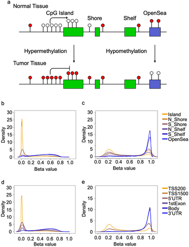
It is well established that cancer-associated DNA methylation alterations occur bidirectionally, but with characteristic patterns occurring in specific genomic regions. For example, CpG Islands and immediately adjacent Shores, are seen to be unmethylated in a wide range of healthy, adult tissues, and frequently acquire methylation in cancer [15]. Other regions, such as Shelves and OpenSeas, are likely to be highly methylated in healthy tissue, and may lose methylation in cancers (Figure 1a). Our thresholds reflect these patterns. Lower thresholds for probes near the transcriptional start site of a gene, or in CpG Islands are overwhelmingly close to zero, while upper thresholds are usually near 0.20 (Figure 1b–e). Conversely, probes in CpG Shelves and OpenSeas, often associated with the gene bodies, 3’UTR and intergenic regions, have upper thresholds close to 1 and a wide range of lower bounds (Figure 1b–e).

Figure 1. Overview of the patterns of DNA methylation across the genome in normal tissues. a) the Central Dogma of DNA methylation: CpG island regions in the promoters of genes classically acquire methylation (solid circles) in tumours, even while DNA methylation is lost (open circles) in CpG open seas. Density plots showing the distribution of thresholds across multiple genomic regions in the normal tissues at the b) lower and c) upper thresholds. Density plots showing the distribution of thresholds at the position to the nearest gene at the d) lower and e) upper thresholds.

Influential reference samples

By design, our thresholds represent the extremes of the reference distribution at each CpG site. In this section, we consider factors that affect threshold values and examine influential samples, i.e., those that sit at the extremes of the distribution for a large number of probes. Beyond individual sample variation, we anticipate that some studies may contribute many influential samples, perhaps due to differences in study design, sample handling, or data processing decisions. In particular, we predict that TCGA samples, which were subject to rigorous QC criteria before processing in centralized facilities using identical protocols, would be more homogeneous than those collected from a variety of datasets on the NCBI’s GEO. Similarly, we anticipate that tissue-specific methylation patterns will drive the threshold values at some CpG sites, and some tissue types may be more influential than others.

To identify influencers, we calculated for each sample, the proportion of CpG sites falling beyond the thresholds. As expected, GEO samples were more likely to influence the thresholds than the TCGA samples (Figure 2a,b and Supplementary Figure S1a-d). In most cases, extreme values were not strongly associated with tissue type. In general, individual studies were a larger source of variation than tissue type (Figure 2c and Supplementary Figure S2a-b). Tissues that were most represented in our reference set, including breast and GI tissue showed large amounts of variation from study to study (Figure 2b and Supplementary Figure S1c-d), and the relative influence of each tissue types were not well correlated between GEO and TCGA (Spearman rho = 0.248; P = 0.492) (Figure 2c).

Figure 2. Box plots show the proportion of outliers contributed by sample in the a) TCGA dataset and b) GEO dataset. c) Scatterplot shows the average proportion of outliers contributed by specific normal tissue types from GEO (x-axis) and TCGA (y-axis).

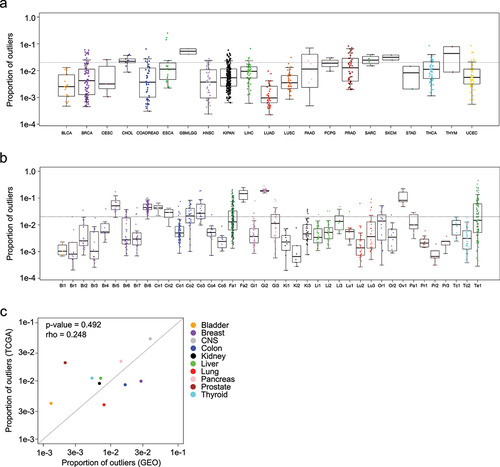
Brain tissue stood out as the exception, with both studies demonstrating high rates of influential samples. We believe this makes sense because of the vast diversity of specialized cell types in the brain [16].

Whole blood

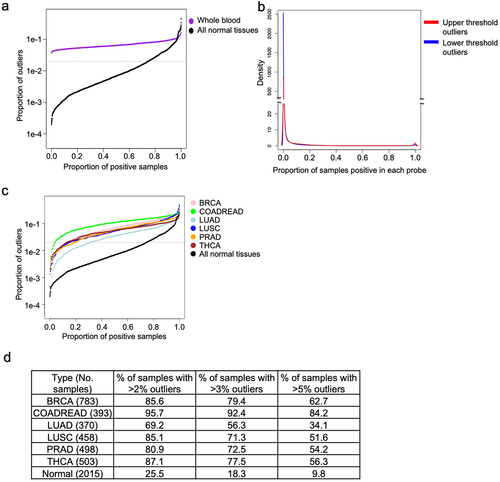
We made the decision to restrict our reference database to solid tissue from healthy patients, and morphologically normal tissue found adjacent to solid tumours, excluding blood which has very distinctive patterns of DNA methylation. The distribution of outliers differed dramatically between whole blood and our normal reference samples (Figure 3a). The distribution is bimodal in whole blood, the vast majority of probes having few outliers, but 2,546 probes were flagged as outliers in every single blood sample (Figure 3b). Gene set analysis of the most commonly outlying markers shows that they are associated with blood cell and immune system biology (Supplementary Table S2).

Figure 3. Characterizing outliers in blood and tumour tissues. a) The proportion of outliers detected in whole blood samples are shown in blue, in contrast to normal refernce tissues, shown in black. Horizontal dotted line is drawn at the selected threshold value of 0.02. b) Density plot showing the proportion of blood samples positive for the full set of outliers. c) Each line shows the proportion of outliers contributed by each sample in multiple tumour types and the normal tissues. Samples are arranged in increasing order, horizontal dotted line is drawn at the selected threshold value of 0.02. d) Table enumerates the proportion of samples in c) with more than 2% (at the dotted line), 3%, and 5% of probes exhibiting outliers.

Aberrant methylation in cancer tissues

Next, we examined the rate and distribution of flagged outliers identified in various tumour types from TCGA, including BRCA, COADREAD, LUAD, LUSC, PRAD and THCA, chosen to span a range of methylation patterns. Results are plotted together with the complete dataset of normal tissues (Figure 3c and Supplementary Figure S2c-d). While a fraction of the tumours of each type have little or no aberrant methylation, every tumour type has many more outliers than normal tissues. Of these 6 tumour types, COADREAD had the greatest proportion of outliers with more than 95% of samples exceeding the expected normal level, while LUAD had the lowest proportion of outliers, with 69.2% of samples meeting the same threshold (Figure 3c,d). Interestingly, we found that some tissue types showed a directional bias. LUSC is the clearest example of this phenomena, as the majority of outliers represent decreases in methylation (Supplementary Figure S2c-d).

Case studies

In the next section, we demonstrate the utility, and limitations, of using methylation outlier calls in place of continuous-valued data, when performing common analysis tasks. The following scenarios represent increasingly complex problems from simple discrimination between tumours and normal tissues, where outlier calls slightly outperforms continuous data, to predicting epigenetic age, where outliers are too crude to capture subtle age-related changes, although they do correlate weakly.

Distinguishing pan-cancer from pan-normal samples

In our first scenario, we consider the relatively simple problem of distinguishing pan-tumour samples (N = 8,378) from pan-normal samples (N = 747) downloaded from TCGA, using both continuous data and flagged outlier data. After partitioning the data into training and test sets, we used logistic regression together with LASSO variable selection [17] to build and test prediction models. When using continuous measures of methylation, a panel of 194 probes distinguished normal samples from tumour tissues with high accuracy (AUC: 0.950; CI: 0.936–0.964; Mann-Whitney P < 0.001) (Figure 4a). A panel of 45 probes, selected the same way, but from the flagged outlier data, performed even better (AUC: 0.978; CI: 0.971–0.984; Mann-Whitney P < 0.001) (Figure 4a). Finally, we flagged outliers from the 194 probes from the continuous model, and retrained the model. Interestingly, the change of accuracy was minor (AUC: 0.927; CI: 0.913–0.942; Mann-Whitney P < 0.001) (Figure 4a) and all 194 sites remained active after the outliers were flagged (i.e., informative because the outliers were non-constant across all samples).

Figure 4. Distinguishing between pan-tumour and pan-normal using flagged outliers and continuous DNA methylation data. a) Receiver Operating Characteristic (ROC) analysis distinguishing pan-tumour from pan-normal tissues with three panels of markers: continuous data, flagged outlier data, and probes selected from continuous data and subsequently flagged for outliers. Heatmap shows the performance of the pan-tumour panels from the b) continuous data c) flagged outlier data, and d) continuous markers that were flagged for outliers after selection.

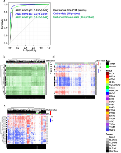
In the tumor tissues from the continuous data, as expected, we observed that probes within the CpG Islands were generally hypermethylated in comparison to the normal tissues (Figure 4b). Furthermore, probes located in OpenSeas tended to be hypomethylated in the tumour tissues in comparison to the normal tissues. Similarly, for the flagged outlier probe panel, in the normal tissues, the outlier probes within the genomic Islands commonly fell above the higher thresholds while probes in OpenSeas frequently fell below the lower thresholds (Figure 4c). In the continuous data probe panel that was flagged for outliers after probe selection, we found that the vast majority of outlier probes were in the tumour tissues (Figure 4d). We also found that the probes that became hypermethylated generally fell above the upper thresholds while the hypomethylated probes mostly fell below the lower thresholds.

Unsupervised clustering of DNA methylation data in lung and kidney tissues

In this more complex scenario, we consider the common problem of sample clustering. To evaluate performance, we selected situations in which the subgroups are known, a slightly artificial but convenient arrangement. The first dataset was comprised of lung tissues, which included lung adenocarcinoma (LUAD) and lung squamous cell carcinoma (LUSC) and normal adjacent tissues from both tumour types. The second dataset was comprised of kidney tissues, which included kidney renal papillary cell carcinoma (KIRP) and kidney renal clear cell carcinoma (KIRC) and normal adjacent tissues from both tumour types. To avoid overfitting, the GEO reference was used to flag outliers in the TCGA lung and kidney datasets, and for both continuous and outlier data, the probes with the greatest 5% standard deviation were used for clustering.

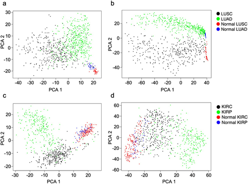
From the lung tissue dataset, we found greater separation of the normal adjacent tissues from tumour tissues with continuous than with outlier data (Figure 5a,b). Conversely, we found that the flagged outlier data clustering showed clearer separation of the lung tumour types in comparison to the clusters made with the continuous data. From the kidney dataset, we observed that the continuous data better captured differences between subtypes both in tumours and in normal adjacent tissues than the outlier data (Figure 5c,d). Interestingly, in both the continuous and flagged outlier data, we saw that the normal adjacent lung and normal adjacent kidney tissues clustered based on the type of adjacent tumour. While continuous data showed a greater ability to cluster the kidney data, overall, the difference in cluster quality between continuous data and outlier data was minimal.

Figure 5. Principal component analysis (PCA) plots show the ability to cluster lung tumours and normal lung tissues with unsupervised a) continuous data and b) flagged outlier data, as well as kidney tumours and normal kidney tissues with unsupervised c) continuous data and d) flagged outlier data.

Flagging outliers using DNA methylation age markers

It is well documented that normal human ageing is accompanied by consistent changes in DNA methylation [17–19]. However, since these changes occur gradually over time, we anticipate that they are often too subtle to cross the threshold and become outliers. To evaluate this hypothesis, we considered a set of 71 age markers identified by Hannum et. al., evaluating them in the same samples in which they were derived (GSE40279) [18], a set of 656 healthy blood samples of individuals with ages ranging between 19–101 years old. A total of 56 of the 71 age markers were available in our reference set and, as expected, the majority of these showed little or no variation across samples, after flagging the outliers. Specifically, in 28% of samples, all 56 age markers fell into the normal range of methylation values, and the vast majority of samples (92%) showed non-normal methylation levels in fewer than 4 markers (Figure 6a–c).

Figure 6. Box plots show the proportion of probes with altered DNA methylation across the different age groups separated by a) the total proportion of flagged outliers, b) the proportion of flagged outliers that cross the upper thresholds and c) the proportion of flagged outliers that cross the lower thresholds. d) the number and percent of active probes calculated for the age probes and non-age probes.

Having observed that age markers are relatively inactive in these samples, producing few outliers, we asked whether they were truly less active than non-age markers. Surprisingly, we found that the percent of active age markers was less than the remaining set of probes, 44.6 and 64.1 respectively, and that this lower number of active markers was statistically significant (Fisher’s exact P = 0.003) (Figure 6d). It is worth noting, however, that while information on chronological age was significantly weaker, it was not wholly absent. Non-normal values were more likely in older individuals (Figure 6a).

Discussion

In this study, we determined probe-specific thresholds for recognizing aberrant DNA methylation on the Illumina methylation array platform. We and others often encounter situations where it is desirable to identify methylation outliers, including when searching for candidate biomarkers, or as an alternative to standard differential analysis when there are insufficient replicate samples for inferential methods. We explored the operating characteristics of those thresholds and tried to provide the reader with guidance on the utility and limitations of our outlier approach by comparing to continuous data in several analyses of increasing complexity.

We downloaded and compiled 25 types of normal, and morphologically normal, tumour-adjacent tissues (2,015 samples) from the TCGA and GEO database. Next, we constructed an R package, OutlierMeth, to determine the DNA methylation thresholds from normal and normal adjacent tissues and to standardize an approach to flag outliers from DNA methylation data. With the use of this package, we characterized flagged outliers in the normal tissue dataset. Except for brain tissue, we did not find strong evidence that a single tissue type contributed a larger influence on the thresholds than other types of normal tissues. The decision to include tumour-adjacent tissue in the reference has both pros and cons. On the one hand, the reference set is compromised as a representation of normal DNA methylation, as field effects have been shown to affect the DNA methylation levels of normal tissue adjacent to tumours [20]. However, we believe that broadening the data collection to include healthy tissue from unhealthy donors is also a strength, capturing a range of risk factors for cancer, as well as co-morbidities that accompany cancer in an ageing population. And while it is not definitive, we are encouraged that we did not find that normal adjacent tissues, all normal tissues from TCGA, contributed a larger influence on thresholds in comparison to the normal tissues, the majority of tissues from GEO. We did however find a large variability in the number of outliers in normal tissues between datasets downloaded from GEO. While the specific reason for this variation remains unknown, it is likely that the differences in tissue handling, the level of cellular heterogeneity and data processing methods contributed to this variation.

We compiled a single reference aggregating multiple solid tissue types, rather than several tissue-specific versions. While specific references would be more accurate, relatively small sample sizes compromise the precision of tissue-specific thresholds in the best of circumstances, and in the absence of any appropriate normal samples, we believe that a conservative, multi-tissue reference will still be useful. And our ability to broadly distinguish tumour tissue from adjacent normal using outliers lends credibility to this idea. On the other hand, our experience with normal blood highlights the limitations of a generic reference. After flagging the outliers in the whole blood dataset, we found that all of the blood samples had outliers in an overlapping set of 2,546 probes. From the gene set analysis, we found that the outliers were located in genes that are known to be important in pathways specific for blood cells.

DNA methylation levels are sensitive to a host of factors beyond tissue and cell type. Genetic variation has been shown to affect DNA methylation and may affect the occurrence of outliers [21]. For example, Mckennan et. al. has shown that DNA methylation in blood cells differs across racial and ethnic groups and that these differences are heavily driven by genetic variants [22]. Likewise, copy number alterations have been reported in multiple types of human tumours, and similar to genetic variants, have been shown to affect DNA methylation [23–26]. Surprisingly, copy number alteration effects on DNA methylation have been found to be minor when comparing normal tissues to a single copy gain or lost [26]. Furthermore, it has been shown that homozygous copy number loss has very little impact on methylation array analysis since these deleted loci are generally removed from the analysis due to the low detection of DNA [26]. While outside the focus of the current study, it would be of great interest to incorporate these and other factors into the outlier model.

When comparing the proportion of outliers between tumour and normal tissues, unsurprisingly, tumour tissues had a larger proportion of outliers than the normal tissues. While most of the tumour tissues tested had a similar ratio of upper and lower outliers, we found that the majority of outliers in the LUSC dataset were in the hypomethylated direction. The cause of the skew for hypomethylated outliers and its biological consequences require further investigation.

After we determined probe-specific thresholds and standardized the approach to flag DNA methylation outliers, we investigated the use of flagged outlier data to address multiple biological study scenarios with different levels of complexity. In the first scenario, we attempted to discover panels of probes that can distinguish pan-tumour from pan-normal samples. We found that the discovered panel of probes using continuous data and outliers were evenly split between hypermethylated and hypermethylated alterations. Furthermore, similar to previous studies, we found that in both types of data, the unmethylated CpG islands in the pan-normal samples mostly become hypermethylated in the pan-tumour samples [2,3]. We also found that the probe panels selected from either continuous and flagged outlier data could accurately distinguish between normal and tumour samples. However, with a smaller number of probes, the flagged outliers showed higher accuracy, as measured by AUC, than the continuous data to distinguish tumour from normal tissues. We also found that the accuracy of the continuous probe panel was unchanged after the data was flagged for outliers. This result suggests that the probes selected to be the most different between pan-tumours and pan-normal in the continuous data were different enough to be flagged as outliers.

In the second scenario, using unsupervised data to subcluster tumour and normal adjacent tissue types, we found that there is a slight advantage in using continuous data over outlier data. Interestingly we found the normal adjacent tissues from the lung and kidney subclustered based on the adjacent tumour type when using either flagged outlier or continuous data. Since array data is generated from bulk tissues, cells in the microenvironment and alterations caused by field effects can affect the DNA methylation values. Previous studies have shown that the cells that make up the microenvironments of the normal tissues adjacent from lung adenocarcinoma and lung squamous cells are different despite being from the same organ [27]. Although untested, we hypothesize that it is microenvironment differences specific to the multiple tumour types that is causing the adjacent normal kidney and adjacent lung tissues to subcluster.

In the third scenario, we flagged outliers from a panel of previously discovered age markers and investigated their ability to distinguish individuals of multiple ages. Although there was a slight increase of outliers that crossed the upper threshold in the older individuals, we found that the majority of information in the age markers was lost after we flagged the data for outliers. This suggests that it may be unwise to flag outliers in data that describes continuous biological events such as ageing. Our results were not unexpected as changes in the peripheral blood have been shown to be continuous across the life course and are generally not of great magnitude [17–19]. While studies have shown that the cellular makeup of the blood can affect the accuracy of epigenetic-based age prediction, further studies are required to better understand the effects of these confounding variables [28,29].

Conclusions

Overall, we made great efforts to determine probe-specific thresholds and to standardize an approach to flag outliers using DNA methylation array data. We also provided a user guide for when to use flagged outliers. Although we believe that the conclusions from this study will largely remain unchanged, further analysis of using probe-specific thresholds to flag aberrant DNA methylation outliers is warranted once more normal tissue samples are analysed with the updated Illumina Epic 850K human methylation array.

Materials and methods

Sample selection

To determine probe-specific thresholds, we compiled normal and tumour adjacent normal samples from public sources. Specifically, we searched the NCBI’s Cancer Genome Atlas project (TCGA) and Gene Expression Omnibus repository (GEO) to identify DNA methylation data on the Illumina 450K human methylation array platform, from normal and morphologically normal tissue adjacent to tumour. More than 2,000 samples, representing 25 normal tissue types were downloaded and compiled to represent the distribution of methylation across the genome. The TCGA dataset used in this study was downloaded from the Firebrowse site (http://firebrowse.org). All available normal adjacent tissues from TCGA were used in this study. The normal tissues from the TCGA were comprised of 21 tissue types and included 747 normal tissue samples. In addition to tumour-adjacent, normal reference samples, methylation data from TCGA tumours were downloaded and used to characterize the operating characteristics of the approach. All other normal tissues and blood samples data were downloaded from the Gene Expression Omnibus (GEO) database (http://www.ncbi.nlm.nih.gov/geo/). We required that the GEO reference dataset description included at least one of the following key words: ‘cancer,’ ‘cancers,’ ‘tumor,’ or ‘tumors’ and had at least 10 normal or normal adjacent samples. All data was downloaded as matrices of already pre-processed beta values, so the collection represents the full range of processing methodologies. A total of 29 datasets, comprising of 15 tissue types and 1,268 normal tissue samples, were compiled from the GEO repository. Pre-processing algorithms varied by study (Supplementary Table S1), and represents the full range of pre-processing practices in the field. Probes at non-CpG targets and sex-associated DNA methylation sites [30] were removed from all data.

Determining thresholds and flagging DNA methylation outliers

Our goal is to identify CpG locations where methylation values are significantly low or high compared to our normal reference samples. Using the standard quantile function in R, we derived upper and lower thresholds at significance levels between 0.01 and 0.00001 for the probes from the Illumina HumanMethylation 450K array for four collections of reference samples: TCGA only, GEO only, TCGA-GEO combined, and blood. Examples of the distribution of normal methylation levels, and corresponding thresholds are shown in Supplementary Figure S3a-d for several individual probes. To flag the outliers for a matrix of methylation values, it is necessary to choose a reference collection and specify the desired threshold level. Values in the normal range are reported as 0 after binarization, while values that lie outside of the selected significance threshold levels for the CpG locus are reported as −1 or 1 depending on direction. The R statistical software suite (version 3.6.0) and custom code was used for all of the analyses in this study [31] and a new R package, OutlierMeth (https://github.com/bdowns4/OutlierMeth), was built for this study and used to flag outliers using the beta values from the Illumina HumanMethylation 450K array. Unless otherwise specified, the reference dataset used in this study was calculated from the TCGA-GEO dataset at the 0.01 significance level.

Methylation outliers in whole blood samples

The decision to use normal and morphologically normal, tumour-adjacent samples to build our reference distributions was motivated by the widespread availability of data from that source and justified by the fact that a large portion of work on DNA methylation takes place in cancer research. This raises the question, however, of whether samples from healthy subjects, and especially from specialized tissues, have unique methylation patterns. To examine this question, healthy whole blood samples, N = 656, was downloaded from GEO (GSE40279) [18]. Gene set analysis, performed with the Wilcoxon rank sum test, was used to interpret differences seen between normal whole blood and reference normal or normal adjacent tissues. Using the same data, we also examined whether epigenetic changes that occur in normal human ageing are large enough to be seen after flagging the outliers. For this purpose, we use a previously published panel of 71 age associated CpG sites [18].

Case study scenarios

To explore the operating characteristics of our flagged outlier methylation data, and evaluate their use and limits, we compare flagged outlier and continuous methylation data in 3 common use cases. These case studies are presented in order of increasing complexity.

Supervised classification of pan-cancer and pan-normal tissues

The idea of the liquid biopsy, a blood test that could detect tumours anywhere in the body, is a true grail of cancer research. For our first use case, we seek candidate markers for such an assay. The pan-tumour and pan-normal datasets were comprised of the complete set of TCGA tumour tissues N = 8,378 and normal adjacent tissues N = 747. The TCGA-GEO reference was used to flag outliers in the pan-tissue datasets. After partitioning the data into training and test sets with the R function sample, we used a logistic regression to model differences between tumours and normal samples. In the discovery dataset, the probes were first sorted by the p-value as calculated by logistic regression using the R function glm. The most significant 1,000 probes were selected and the R package glmnet function LASSO was used to select the panel of probes that were analysed in the testing dataset [17]. The R function glm predict was used to classify the samples in the testing dataset. The R package pROC was used to make the receiver operator characteristic (ROC) plot and to calculate the area under the curve (AUC) and 95% confidence interval (CI) [32]. The R package pheatmap was used to generate all heatmaps [33]

Unsupervised clustering analysis of lung and kidney tissues

Clustering analysis is commonly used to identify molecularly distinct tumour subtypes, among other tasks. We implement a version of that analysis here, using two cancers with well characterized subtypes. The scenario is slightly artificial in that the subgroups are already known, but there is an advantage in the ability to compare the results to the truth. The TCGA lung dataset was comprised of lung squamous cell carcinoma (LUSC); tumours N = 370 and normal adjacent tissues N = 41 and lung adenocarcinoma (LUAD); tumours N = 458 and normal tissues N = 32). The kidney dataset was comprised of kidney renal clear cell carcinoma (KIRC); tumours N = 319 and normal adjacent tissues N = 160 and kidney renal papillary cell carcinoma (KIRP); tumours N = 275 and normal adjacent tissues N = 45. To avoid data overfitting, the GEO reference was used to flag the outliers in the lung and kidney datasets. The R function sd was used to calculate the standard deviation for each of the probes and the top 5% of the probes with the greatest standard deviation were used for clustering. Sample and probe similarity was measured using the L² distance, calculated with the R function dist, and the function Cmdscale was used to scale the distance values for principal components analysis.

Acknowledgments

The authors would like to thank Dr. Hariharan Easwaran for his generous advice for the preparation of this manuscript.

Disclosure statement

No potential conflict of interest was reported by the authors.

Data availability statement

Data from TCGA were downloaded from the website Firebrowse.org (Supplementary Table S1) shows GSE study IDs of all data downloaded from the GEO omnibus.

Supplementary material

Supplemental data for this article can be accessed online at https://doi.org/10.1080/15592294.2023.2213874

Additional information

Funding

This work was supported by the DOD-BCRP postdoctoral fellowship under grant W81×WH1810482 to BD

References

- Jones PA, Takai D. The role of DNA methylation in mammalian epigenetics. Science. 2001;293(5532):1068–14.
- Baylin SB. DNA methylation and gene silencing in cancer. Nat Clin Pract Oncol. 2005;2(Suppl 1):S4–11.
- Wittenberger T, Sleigh S, Reisel D, et al. DNA methylation markers for early detection of women’s cancer: promise and challenges. Epigenomics. 2014;6(3):311–327. DOI:10.2217/epi.14.20
- Barros-Filho MC, Dos Reis MB, Beltrami CM, et al. DNA methylation-based method to differentiate malignant from benign thyroid lesions. Thyroid: Offic J Am Thyroid Association. 2019;29(9):1244–1254. DOI:10.1089/thy.2018.0458
- Beltrami CM, Dos Reis MB, Barros-Filho MC, et al. Integrated data analysis reveals potential drivers and pathways disrupted by DNA methylation in papillary thyroid carcinomas. Clin Epigenetics. 2017;9:45.
- Johnson KC, Houseman EA, King JE, et al. Normal breast tissue DNA methylation differences at regulatory elements are associated with the cancer risk factor age. Breast Cancer Res. 2017;19(1):81.
- Vrba L, Futscher BW. A suite of DNA methylation markers that can detect most common human cancers. Epigenetics. 2018;13(1):61–72.
- Wang Z, Wu X, Wang Y. A framework for analyzing DNA methylation data from Illumina Infinium HumanMethylation450 BeadChip. BMC Bioinf. 2018;19(Suppl 5):115.
- Zhang J, Fan J, Wang P, et al. Construction of diagnostic and subtyping models for renal cell carcinoma by genome-wide DNA methylation profiles. Transl Androl Urol. 2021;10(11):4161–4172. DOI:10.21037/tau-21-674
- Tang W, Wan S, Yang Z, et al. Tumor origin detection with tissue-specific miRNA and DNA methylation markers. Bioinformatics. 2018;34(3):398–406.
- Fackler MJ, Lopez Bujanda Z, Umbricht C, et al. Novel methylated biomarkers and a robust assay to detect circulating tumor DNA in metastatic breast cancer. Cancer Res. 2014;74(8):2160–2170. DOI:10.1158/0008-5472.CAN-13-3392
- Chen C, Huang X, Yin W, et al. Ultrasensitive DNA hypermethylation detection using plasma for early detection of NSCLC: a study in Chinese patients with very small nodules. Clin Epigenetics. 2020;12(1):39. DOI:10.1186/s13148-020-00828-2
- Liu MC, Oxnard GR, Klein EA, et al. Sensitive and specific multi-cancer detection and localization using methylation signatures in cell-free DNA. Ann Oncol. 2020;31(6):745–759.
- Downs BM, Ding W, Cope LM, et al. Methylated markers accurately distinguish primary central nervous system lymphomas (PCNSL) from other CNS tumors. Clin Epigenetics. 2021;13(1):104. DOI:10.1186/s13148-021-01091-9
- Baylin SB, Jones PA. Epigenetic determinants of cancer. Cold Spring Harb Perspect Biol. 2016;8(9):a019505.
- Capper D, Jones DTW, Sill M, et al. DNA methylation-based classification of central nervous system tumours. Nature. 2018;555(7697):469–474. DOI:10.1038/nature26000
- Friedman J, Hastie T, Tibshirani R. Regularization paths for generalized linear models via coordinate descent. J Stat Softw. 2010;33(1):1–22.
- Hannum G, Guinney J, Zhao L, et al. Genome-wide methylation profiles reveal quantitative views of human aging rates. Mol Cell. 2013;49(2):359–367. DOI:10.1016/j.molcel.2012.10.016
- Bocklandt S, Lin W, Sehl ME, et al. Epigenetic predictor of age. PLoS ONE. 2011;6(6):e14821. DOI:10.1371/journal.pone.0014821
- Teschendorff AE, Gao Y, Jones A, et al. DNA methylation outliers in normal breast tissue identify field defects that are enriched in cancer. Nat Commun. 2016;7:10478.
- Smith AK, Kilaru V, Kocak M, et al. Methylation quantitative trait loci (meQtls) are consistently detected across ancestry, developmental stage, and tissue type. BMC Genomics. 2014;15:145.
- McKennan C, Naughton K, Stanhope C, et al. Longitudinal data reveal strong genetic and weak non-genetic components of ethnicity-dependent blood DNA methylation levels. Epigenetics. 2021;16(6):662–676. DOI:10.1080/15592294.2020.1817290
- Berger AC, Korkut A, Kanchi RS, et al. A comprehensive pan-cancer molecular study of gynecologic and breast cancers. Cancer Cell. 2018;33(4):690–705.e9. DOI:10.1016/j.ccell.2018.03.014
- Network CGAR. Comprehensive genomic characterization of squamous cell lung cancers. Nature. 2012;489(7417):519–525.
- Network CGA, Akdemir K, Aksoy B. Genomic classification of cutaneous melanoma. Cell. 2015;161(7):1681–1696.
- Feber A, Guilhamon P, Lechner M, et al. Using high-density DNA methylation arrays to profile copy number alterations. Genome Biol. 2014;15(2):R30. DOI:10.1186/gb-2014-15-2-r30
- Lambrechts D, Wauters E, Boeckx B, et al. Phenotype molding of stromal cells in the lung tumor microenvironment. Nat Med. 2018;24(8):1277–1289. DOI:10.1038/s41591-018-0096-5
- Zhang Q, Vallerga CL, Walker RM, et al. Improved precision of epigenetic clock estimates across tissues and its implication for biological ageing. Genome Med. 2019;11(1):54. DOI:10.1186/s13073-019-0667-1
- Chen BH, Marioni RE, Colicino E, et al. DNA methylation-based measures of biological age: meta-analysis predicting time to death. Aging. 2016;8(9):1844–1865. DOI:10.18632/aging.101020
- Suderman M, Simpkin A, Sharp G, et al. Sex-associated autosomal DNA methylation differences are wide-spread and stable throughout childhood. bioRxiv. 2017;2017(2017):118265.
- Dowle M, Srinivasan A, Short T. data.table: Extension of 'data.frame'. R Package. 1(8). 2019.
- Robin X, Turck N, Hainard A, et al. pROC: an open-source package for R and S+ to analyze and compare ROC curves. BMC Bioinf. 2011;12:77.
- Kolde R. Pheatmap: pretty heatmaps. R Package version 2012;1(2): 726.