A Decentralized Robust PID Controller Design for the Shape Control of a Magnetic Fluid Deformable Mirror

Abstract

This article presents a systematic approach to the design of a decentralized robust PID controller to regulate the surface shape of a magnetic fluid deformable mirror (MFDM). The proposed approach offers the simplicity of the decentralized controller implementation while accounting for robustness and performance constraints. The controller design problem is formulated as a multi-objective H _∞/H ₂ static output feedback problem. The desired controller is obtained by iteratively solving properly formulated linear matrix inequalities (LMIs). Finally, the experimental evaluation of the proposed controller performance on a MFDM-based adaptive optics system illustrates the effectiveness of the proposed MFDM surface shape control approach.

Keywords:

• adaptive optics
• linear matrix inequalities (LMIs)
• magnetic fluid deformable mirror
• PID control
• robust control

NOMENCLATURE

AO	=	adaptive optics
DC gain	=	gain of the system with respect to static inputs
DM	=	deformable mirror
e	=	performance variable
F	=	static output feedback gain
G	=	system consisting of the wavefront corrector, a gain of 2, and the wavefront sensor
G 0	=	DC gain of the system G
	=	DC decoupled plant G (i.e., )
	=	diagonal entry in
‖·‖∞	=	H ∞ norm of a system
‖·‖2	=	H 2 norm of a system or L 2 norm of a signal
I	=	identity matrix
K	=	controller
K PID	=	PID controller
k PID	=	diagonal entry in K PID
LMI	=	linear matrix inequality
L 2	=	set of square integrable functions
MFDM	=	magnetic fluid deformable mirror
MIMO	=	multi-input multi-output
PID	=	proportional+ integral+ derivative
r	=	reference signal
S 0	=	sensitivity function of the closed loop system
s 0	=	diagonal entry in S 0
SISO	=	single-input single-output
u	=	vector of current inputs to the wavefront corrector
WFC	=	wavefront corrector
W	=	MIMO low-pass filter
w	=	SISO low-pass filter
w Δ(s)	=	bandpass filter
y	=	vector representing the spatially sampled surface shape of the measured wavefront
y p	=	vector representing the spatially sampled surface shape of the mirror
Δ	=	constant uncertainty matrix
	=	additive uncertainty in the representation of
λ	=	wavelength of the light
ζ m	=	mirror surface shape
ζ r	=	shape of the wavefront of the light beam reflected from the mirror
τ	=	time delay associated with the wavefront sensor model
Σ	=	nominal unforced closed loop system
	=	state space representation of the plant in the closed loop system static output feedback configuration
	=	state space representation of the closed loop system in a static output feedback configuration
	=	state space representation of the system
	=	state space representation of the system
	=	state space representation of the system w
	=	state space representation of the system w Δ
ω	=	frequency (rad/s)

1. INTRODUCTION

Adaptive optics (AO) systems are used to cancel the adverse effects of high-order, time-varying optical aberrations on the quality of images provided by high-resolution imaging systems. They were initially developed for applications in astronomical imaging systems where they were used to compensate for the effects of atmospheric turbulence on the resolution of the images of distant stellar bodies provided by ground-based telescopes (Tyson, 2000; Hardy, 1998). Recent advancements in the AO technology have led to its application in systems ranging from those used in free-space communication to those used in retinal imaging applications.

AO systems make use of active optical elements called wavefront correctors (WFCs) to compensate for the high-order, time-varying optical aberrations. Deformable mirrors (DMs) characterized by a deformable reflective surface are the most common type of WFC (Doble and Miller, 2006). Magnetic fluid deformable mirrors (MFDMs) are a novel type of DMs developed by coating the free surface of a magnetic fluid with a reflective film. Since the shape of the resulting reflective surface can be deformed using a magnetic field generated by electromagnets placed under the fluid volume, it serves as an effective WFC. The main advantages of these liquid mirrors are their low cost since they are easy to fabricate, the high optical quality of their reflecting surface (Borra et al., 2006), and their ability to provide very large strokes (several tens of micrometers) (Laird et al., 2004; Brousseau et al., 2006).

Despite these advantages, the use of MFDMs in practical applications has been limited because of difficulties in controlling the surface shape of these mirrors. A major source of these difficulties is the nonlinear response of the mirror surface to the magnetic field applied to control its shape. Recently, a new MFDM design was proposed to solve this problem, where the magnetic fluid as well as the array of electromagnetic coils are placed inside a uniform magnetic field generated using a Helmholtz coil (Iqbal and Ben Amara, 2008). The novel design approach helps linearize the response of the MFDM surface to the applied magnetic field and thus allows the use of linear control algorithms to control the mirror surface shape. This modified design method makes the application of the MFDM mirrors in practical AO systems possible. For example, one of the potential applications of MFDMs is in adaptive optic ophthalmic imaging systems (Doble and Miller, 2006). Another major application could be in optical testing with aspheric surfaces, which are widely used in inexpensive cameras and optical disk players, because of their low cost and high performance (Pruss and Tiziani, 2004). Such tests make use of null lenses to precisely match the test light wavefront shape to the aspheric shape of the surface being tested. The instant reshaping of the surface of the MFDM offers more flexibility and cost savings in using and adapting null lenses as compared to fabricating a whole set of static null lenses for different aspheric shapes of the surface being tested.

Utilizing the design modification mentioned above, the first-ever experimental evaluation of a closed-loop adaptive optics system based on MFDMs was presented in Iqbal et al. (2009). A closed loop system comprising the novel modified MFDM was controlled using the influence function based control method widely adopted in the AO community. The controller was designed based on the assumption that the mirror can be represented using its DC gain (representing the response of the mirror to constant unit step inputs) obtained using the developed analytical model of the mirror in Iqbal and Ben Amara (2008). The multi-input multi-output (MIMO) wavefront corrector model can then be fully decoupled by including the inverse of the DC gain as part of the controller. A decentralized PI controller is then designed simply based on the decoupled system. However, the MFDM usually exhibits significant dynamics even in the low frequency range. Therefore, the approximation of the plant model by a static DC model introduces modeling errors whose effects become more pronounced as the system operating frequency increases. These modeling errors may eventually lead to instability in the resulting closed loop system. A possible solution to address this problem is to design the controller based on the full plant model. In Iqbal et al. (2010), a mixed sensitivity H _∞ controller was proposed to provide good tracking performance of the mirror surface in the desired frequency range. However, from a practical point of view, the design of this type of controllers becomes more and more difficult as the number of actuators increases, and the resulting controller becomes also increasingly computationally demanding. As a middle ground between the two solutions presented above, this article presents a decentralized robust PID controller design method for the MFDM shape control. The proposed controller maintains the computational and implementation simplicity of the PID controller considered in Iqbal et al. (2009) but at the same time addresses the modeling uncertainties and provides the desired tracking performance in the closed loop system for static or slowly varying reference signals. In the design of the decentralized controller, a decoupled approximate dynamic model of the WFC is first obtained (as opposed to the static model considered in Iqbal et al., 2009). Then, based on the resulting decoupled system model, a robust PID controller design approach is employed to ensure the system stability in the whole range of operating frequencies is maintained, while also achieving the desired tracking performance in the closed loop system with respect to static or very slowly time-varying shapes of the mirror surface. Given the fixed structure of the PID controller, the design problem is first converted into a multi-objective H _∞/H ₂ static output feedback problem. In this new formulation, the controller to be designed is a static controller represented by the gains of the desired PID controller (Cao et al., 1998). The desired controller parameters are then obtained by iteratively solving some properly formulated linear matrix inequalities. The performance of developed control algorithm is evaluated on an adaptive optics system involving a prototype MFDM. The experimental results indicate the effectiveness of the proposed controller in tracking the desired shapes for the MFDM surface. It should be noted that the controller design approach presented in the article is not restricted to magnetic fluid deformable mirrors, and is applicable to various other deformable mirror designs, such as for example electrostatically or electromagnetically actuated membrane mirrors.

The rest of the article is organized as follows. The magnetic fluid mirror and the corresponding AO system description are presented in Section 2. In Section 3, a decentralized robust PID controller design method is proposed, where the robust stability constraint and the desired control performance constraint are formulated in a mixed H _∞/H ₂ static output feedback problem. A corresponding controller synthesis algorithm is then proposed by iteratively solving properly formulated linear matrix inequalities. Results on the experimental investigation of the performance of proposed algorithm in an adaptive optics system involving a prototype MFDM are presented in Section 4, followed by the conclusion in Section 5.

2. SYSTEM DESCRIPTION

MFDMs can potentially be implemented in numerous industrial applications, such as dynamic null lenses for aspheric surface testing (Pruss and Tiziani, 2004), where the surface shape of the MFDM can be adjusted easily as a reference aspheric shape that adapts to the individual aspheric surface under testing. In this article, an adaptive optic system setup with a prototype MFDM will be used to evaluate the proposed robust PID design method for producing desired reference mirror surface shapes. A simple schematic diagram of the system setup is shown in Figure 1. The main components of the AO system include a wavefront sensor, a wavefront corrector (MFDM) and a controller. A laser beam with planar wavefront is directed to the surface of the MFDM. The light reflects back from the surface of the MFDM as a beam having an aberrated wavefront—the aberrations being induced by the surface shape of the MFDM. The aberrated beam is then detected by the wavefront sensor. Based on the measured feedback signals, a control system computes the appropriate command signals for the MFDM to deform the shape of the mirror surface such that the measured aberrations in the wavefront of the reflected beam match the desired aberrations. With the traditionally designed MFDM it is well known that the surface shape control of MFDMs using linear control algorithms is very difficult. These difficulties arise mainly due to the nonlinear mirror surface shape response to the applied magnetic field. A modified design of a MFDM, which superimposes a uniform vertical magnetic field on the magnetic field of the array of electromagnetic coils, was proposed in Iqbal and Ben Amara (2008). The design modification allows for the linearization of the response of the MFDM to the applied magnetic field generated by the actuators. The corresponding analytic linear model of the response of the surface shape of the MFDM is also developed in Iqbal and Ben Amara (2008), and can be written in state space form as:

Figure 1 Operating principle of an adaptive optics system. In this setup, the deformable mirror shape is adjusted so that the wavefront shape of the beam reflecting off the deformable mirror surface matches a desired shape stored in the controller. (Figure is provided in color online.).

where x _p ∈ ℝ ⁿ is the vector of state variables, y _p ∈ ℝ ^m is the vector of MFDM surface shape displacements, u ∈ ℝ ^l is the vector of control currents applied to the electromagnetic actuators, A _p , B _p and C _p are the system matrices. The MFDM model considered in this paper is a MIMO system with l = m = 19 where the 19 input electromagnetic coils are arranged in a circular pattern and the output mirror surface deflections are measured immediately above the center of each of the 19 electromagnetic coils.

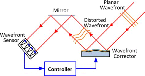
The vector of control currents u applied to the wavefront corrector results in a mirror surface shape ζ _m . Let ζ _r denote the shape of the wavefront reflected from the mirror and sensed by the wavefront sensor, where ζ _r  = 2ζ _m , i.e., the reflected wavefront shape is twice of the mirror surface shape (Hampson, 2008; Baudouin et al., 2008). The sensor samples the wavefront ζ _r at discrete locations—using an array of lenslets in the case of the Shack–Hartmann wavefront sensor. The sampled wavefront shape information, expressed as a vector y ∈ ℝ ^m of discrete displacements, is provided to the controller which computes the actuator currents u ∈ ℝ ^l to be applied to the array of l input actuators. Since the main objective of the research work presented in this article is to demonstrate the ability to control a MFDM in closed-loop operation to produce a desired reference shape, the currents are computed in the controller such that the measured aberration y is equal to the desired reference aberration r. The block diagram of the resulting closed-loop AO system is shown in Figure 2 where K is the controller and G is an augmented plant consisting of the wavefront corrector, a static gain of 2, and the wavefront sensor.

Figure 2 Block diagram of the closed-loop adaptive optics system experimental setup. (Figure is provided in color online.).

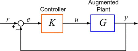
To develop a model of the augmented plant G, the sensor is represented using a time delay τ. Hence, the overall plant model is G(s) = 2e ^{−τ s} P(s). In this configuration, the controller K is required to provide input currents u such that the measured output signal y, representing twice the shape of the deformable mirror surface, tracks the specified reference surface r, i.e., the magnitude of the performance error e = r − y is minimized.

3. DECENTRALIZED ROBUST PID CONTROLLER DESIGN

In this section, a decentralized PID controller design is proposed to control the shape of the MFDM. A PID controller is considered since its has a very simple structure with only three gains to tune. To further simplify the design and implementation of the PID controller, a decentralized structure of the controller is considered where the control signal applied to a given actuator is generated based only one error signal associated with the spatial location of the actuator. To design a decentralized controller for the MFDM, an approximate decoupled dynamic model of the plant is considered, and is obtained using three main steps. The first step involves choosing collocated actuation and sensing points on the mirror. Hence each measurement is maximally influenced by the input from the actuator at the same spatial location, and the influence of the other actuator inputs is minimized. In the second step, the plant model is decoupled at DC by cascading the inverse of the DC gain of the plant model, as part of the controller, with the plant. The third step involves discarding the off-diagonal entries in the system resulting from cascading the inverse of the DC gain of the plant with the plant model. Since the accuracy of the resulting model starts to deteriorate with the increasing operating frequency, a robust controller design approach is employed to ensure the closed loop system stability. The PID controller structure ensures that the MFDM can successfully track desired static or slowly time-varying surface shapes while providing a fast transient response that is acceptable from a practical point of view. This latter goal is achieved by designing the controller to minimize the L ₂ norm of the mirror shape tracking error. In the following, the problem of designing the decentralized robust controller with a PID structure is formulated as an optimization problem which is solved using linear matrix inequalities (LMIs) approach.

3.1. Decoupling of the Plant Model

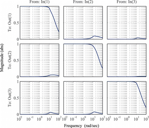
As predicted by the analytical model P(s) and experimentally validated in Iqbal and Ben Amara (2008), the surface shape generated by a single coil features a Gaussian profile, with the peak surface deflections obtained immediately above the center of the coil. When observed in the context of the linear response of the MFDM, which allows the surface deflection at any point to be measured as the summation of the influence of all active coils, this feature allows the MIMO MFDM system to be decoupled and represented as a collection of single-input single-output (SISO) systems. Specifically, if surface deflections obtained immediately above the centers of the input electromagnetic coils are used as the measured output for the control signal computations, the coupling among different input-output channels is minimal. For the 19-input channel system, 19 output points in the measured pupil are chosen such that each of the output points corresponds to the location of an input coil. This arrangement ensures that each output point is influenced maximally by one input coil only i.e., the one immediately underneath the point, while the effect of the other inputs is significantly small. The decoupling effect can be clearly observed from the Bode magnitude plot of the MFDM system as shown in Figure 3 where magnitudes in the plots on the leading diagonal are significantly higher than those placed off-diagonal. The figure shows the Bode plots for three selected channels along the radial direction in the wavefront corrector. Due to symmetric arrangement of the input coils, the three selected channels sufficiently represent the whole 19-input-19-output system.

Figure 3 Bode plot of the MFDM. The array of Bode plots shows the system response for channels corresponding to three inputs and three outputs selected in a radial direction. The plots on the diagonal correspond to collocated input-output pairs. (Figure is provided in color online.).

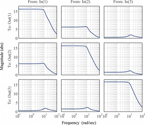
Although the right choice of input-output points does produce the desired decoupling effect, the system is still not fully decoupled. For example, the coupling between the adjacent output points (1 and 2, for instance) is of the order of 20% (i.e., the magnitude of the surface deflection at the output point 2 due to an input applied at coil 1 ≈ 0.2 times the magnitude of the deflection at the output 1 due to the input applied at coil 1). Therefore, some means to further reduce the coupling effect are still needed.

A further insight into the Bode plot of the plant model P(s) reveals that the magnitude of the surface displacements remains constant over a range of low frequencies. This implies that the MFDM can be considered as a static system in this range of frequencies. Since a static MIMO system can be fully decoupled using the DC gain of the system (Skogestad and Postlethwaite, 2004), this property of the MFDM is exploited to further improve the decoupling effect imparted by the choice of output points as described above.

The DC gain G ₀ of the augmented plant G(s) was obtained as G ₀ = G(0). For the frequency range 0 < ω < 7 rad/s, the following relationship holds:

where I is a 19 × 19 identity matrix. It follows from (2) that for 0 ≤ ω ≤ 7 rad/s the augmented system is a DC decoupled system represented by a unit gain delay system e ^{−τ s} over each of the decoupled channels. This DC decoupling effect can be incorporated in a closed loop system by simply adding before the plant G in the closed-loop system as shown in Figure 4, where K _PID represents the controller to be designed in the following section.

Figure 4 Block diagram of the closed-loop system showing the system . (Figure is provided in color online.).

The DC decoupling effect can be more clearly observed by re-drawing the Bode plot of the same system as was shown in Figure 5, now after multiplying the system model with the inverse of its DC gain G ₀. It is evident from the magnitude plot in Figure 5 that the system is significantly decoupled in the low frequency range 0 ≤ ω ≤ 7 rad/s. The decoupling allows the closed-loop system to be treated as a collection of multiple SISO systems each of which is controlled independently by a controller k _i , i = 1, 2,…, l. However, it can be seen that the decoupling starts to deteriorate with the increasing operating frequency, Therefore, in the following, a robust decentralized PID controller design approach is employed to ensure the system stability in the whole operating frequency range, while also achieving the desired tracking performance in the closed loop system.

Figure 5 Bode plot of the DC decoupled MFDM system. The system is DC decoupled by pre-multiplying it with the inverse of its DC gain. (Figure is provided in color online.).

3.2. Controller Design

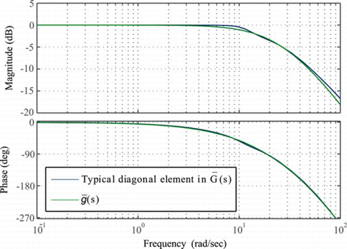
For the system under consideration, the use of the DC gain matrix serves well in decoupling the different channels in the low frequency range. As indicated by the selected Bode magnitude plots shown in Figure 5, the diagonal entries represent the most significant entries in the augmented system , whereas the contribution of the other entries is much less significant. Moreover, the diagonal entries in are all similar. Hence these diagonal entries can all be represented using the same function . Therefore, is represented as

The function can be approximated using a dynamic model given by

where approximates each of the diagonal entries in as a second order system, assuming there is no time delay, and is the Pade approximation of the sensor delay transfer function e ^{−τ s} , with τ = 0.0345 sec. Figure 6 shows a comparison of the Bode plots of and one of the diagonal entries in . The comparison indicates that provides an accurate representation of the diagonal entries in . The off-diagonal entries in (3) denote the less significant uncertain dynamics in the decoupled system . Based on in (4), then can be reformulated as

Figure 6 Bode plots of and that of a typical diagonal entry in . (Figure is provided in color online.).

where represents the additive model uncertainty. In order to simplify the design of the PID controller, the uncertainty term will be represented using a constant matrix Δ weighted by a band pass filter w _Δ(s) as

where Δ ∈ ℝ ^m×l is such that all entries δ ^ij , i = 1,…, m, j = 1,…, l in Δ satisfy − ρ ≤ δ _ij  ≤ ρ and where ρ can be determined experimentally.

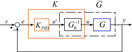
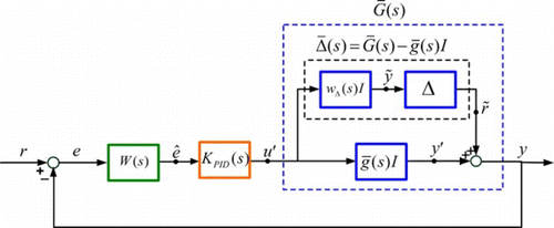
In the following, a robust PID controller will be developed for the augmented system (5). First, in order to eliminate the high frequency noise in the real system, the filter given by W(s) = w(s)I, where w(s) is a low pass filter transfer function, will be applied to the error signal e. By considering a decentralized PID controller of the form K _PID = k _PID I, it follows that the nominal closed loop system is fully decoupled. The resulting closed loop system is shown in Figure 7.

Figure 7 Block diagram of the closed-loop system with the uncertain plant model. (Figure is provided in color online.).

For the purpose of stability robustness analysis, the signal r is set to zero first and the closed loop system block diagram is redrawn as shown in Figure 8, where Σ is the system with input and output . The system Σ is given by

Figure 8 Block diagram of the reconfigured closed loop system showing the blocks Δ and Σ. (Figure is provided in color online.).

where S ₀ is the sensitivity function given by

Let . Then we have

Assuming Σ is stable, then the robust stability of the closed loop system shown in Figure 8 is satisfied if (Zhou et al., 1995)

which is equivalent to

Let J ∈ R ^M×L be such that all its entries are equal to or less than one. Then ‖Δ‖ ≤ ρσ_max(J), where σ_max(J) denote the maximum singular value of J. Based on (9), it follows that ‖Σ‖_∞ = ‖w _Δ k _PID ws ₀‖_∞. Let , then the robust stability condition of the closed loop system can be written as

If (11) is satisfied, then the designed PID controller yields a stable closed loop system. However, the regulation performance of the closed loop system is not considered yet since the design is based only on the stability robustness constraint (11). In the following, the convergence rate of the closed loop system with respect to the static inputs is performed by minimizing an H ₂ performance specification. Consider the nominal closed loop system subject to an input r = v1 _d , where v ∈ ℝ ^m is a constant vector and 1 _d is the scalar valued unit step function. An additional controller design objective is considered where it is desired to find a PID controller K _PID that minimizes the L ₂ norm of e, i.e., ‖e‖₂, by considering only the nomial system in the closed loop system (i.e., without considering the uncertainty . Since the sensitivity function S ₀ relates the input r to the error e, the solution of this design constraint can be obtained by considering a standard H ₂ optimal control problem where it is desired to minimize the H ₂ norm of the system . In order to avoid the unstable pole introduced by , the system can be approximated by the system , where α is a small positive constant. Therefore, the decentralized robust PID controller design problem is converted into a mixed H ₂/H _∞ multiobjective design problem as

In the following, the above optimization problem is first expressed as a mixed H ₂/H _∞ static output feedback problem. A synthesis algorithm based on solving iterative linear matrix inequalities (ILMIs) is then developed to find a suboptimal solution to this nonconvex problem. Consider the ith channel of the closed loop system in Figure 7. Write the following state space representation for

where is the vector of state variables, is the ith control input, y _i ∈ ℝ is the ith output displacement, , , and are the corresponding system matrices. A state space representation for w(s) is given as follows:

where x _w is the vector of state variables, e _i  = r _i  − y _i ∈ ℝ is the ith performance error, is the ith output of the filter, A _w , B _w , and C _w are the corresponding system matrices. Similarly, the weight function w _Δ(s) and are represented, respectively, as

and

where x _Δ and x _s are the vector of state variables, A _Δ, B _Δ, C _Δ, and D _Δ are the corresponding system matrices. The control signal generated by the PID controller k _PID is given by

where k _p , k _i , k _d ∈ ℝ are the parameters to be designed. Let , where χ₁ = x _g , χ₂ = x _w , χ₃ = x _Δ, χ₄ = x _s , . It follows that

Define the new output variables , where , , and , and the new performance variable , then the state space representation from and r _i to and can be written as

where , , , , , , and . Therefore, with respect to the system (17), the design of the PID controller is converted into a static output feedback controller design problem where the control signal is given by and where . Hence, the controller design problem is cast as a mixed H ₂/H _∞ static output feedback controller design problem for the system (17) based on solving the optimization problem (12). Using the static output feedback controller F, the state space representation of the closed loop system involving the modified plant (17) becomes

It should be noted that the H _∞ norm of the closed loop system relating to z _∞ (i.e., to is the same as that of the closed loop system Σ _{r i , z ∞} in (18) relating r _i to z _∞. Also, is the same as the H ₂ norm of the closed loop system Σ _{r i , z 2} in (18) relating r _i to z ₂ (i.e., to . Consequently, the design of the PID controller presented in the following is based on considering ‖Σ _{r i , z ∞} ‖_∞ and ‖Σ _{r i , z 2} ‖₂. Hence, the mixed H ₂/H _∞ static output feedback problem can then be cast in the form of an optimization problem involving matrix inequalities as (Scherer et al., 1997):

where and P > 0. Since the above matrix inequalities are nonlinear in the unknown parameters , P and F, they cannot be solved directly using LMI solvers. In the Appendix, an algorithm is proposed to obtain a solution for OP1 by iteratively solving a set of properly formulated linear matrix inequalities.

4. EXPERIMENTAL RESULTS

In this section, the performance of the proposed PID controller is experimentally evaluated using a prototype MFDM incorporated as part of an AO setup. The decentralized robust PID controller is implemented on the experimental setup given by the schematic layout shown in Figure 9. A detailed description of the system can be found in (Iqbal et al., 2009).

Figure 9 Layout of the experimental setup (L: lens, M: mirror, R: relay, BS: beam-splitter, all dimensions are in mm). The items in dotted blue lines are needed only for retinal imaging applications. (Figure is provided in color online.).

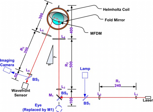
First the decentralized robust PID controller is designed based on the plant model G(s) obtained using the proposed analytical modeling method in Iqbal and Ben Amara (2008). The model represents a prototype 19-channel MFDM used in the experimental setup. The wavefront surface shape y ∈ ℝ¹⁹ is measured vertically above the locations of the input coils. For the 19-input-19-output system, based on Bode plot analysis of the decoupled system, we have ρ ≤0.15 and each output is mostly affected by the neighbor actuators. Based on the modeling data, we obtain ‖Δ‖_∞ ≤ 0.9 and the uncertain weight function w _Δ as

The low pass filter w(s) is selected as

Using these parameters, the proposed iterative algorithm provides the following PID controller

The resulting PID controller was discretized using Tustin's approximation algorithm. The performance of the PID controller is tested by tracking a surface shape formed by the following set constant deflections:

which forms a generalized aspheric surface shape. Figure 10a shows the time history of the wavefront shape measured at the 19-points coinciding with the location of the coils. The RMS error in tracking the reference shape is also given in Figure 10b. The experimental results show a residual steady-state error of 0.0636 µm (where λ = 661 nm is the wavelength of the laser light). As a comparison with the performance of the control systems presented in Iqbal et al. (2009, 2010), it should be noted that with respect to the reference signal given by r _o , the rms error values were 0.08 µm in Iqbal et al. (2009) and 0.092 µm in Iqbal et al. (2010). Hence it can be seen that with an rms error value of 0.063 µm, the proposed controller provides a superior performance to the controllers presented in Iqbal et al. (2009, 2010). Figure 11 shows the contour plot of the error surface i.e., the difference of the reference surface shape and the measured wavefront shape. The reference surface shape used here is the surface obtained by fitting the discrete reference displacements r _o to a linear combination of the first 15 Zernike polynomials.

Figure 10 Experimental tracking of the static reference shape using the decentralized PID controller. (Figure is provided in color online.).

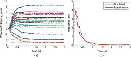
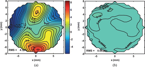
Figure 11 Contour plot of the error surface in µm. (a) Before correction (b) After correction. (Figure is provided in color online.).

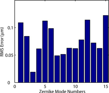
The Zernike modes present a complete set of basis functions that can be used to represent any desired surface shape using a linear combination of these modes. The number of Zernike modes that the mirror surface can produce is a good estimate of the spatial resolution of the wavefront correction offered by the mirror. Therefore, the closed-loop system comprising the proposed controller and the prototype MFDM was tested for its ability to generate a series of Zernike mode shapes. Figure 12 shows the results where the surface plots of the first 15 Zernike modes are shown as desired shapes and are compared to the shapes obtained using the closed loop system. The difference is shown as an error surface for each mode shape. The RMS of the error surfaces is plotted in Figure 13. The RMS error values are computed only at the 19 control points since the number of actuators used in the prototype is small and computing the RMS error over the whole surface will not in this case be reflective of the capabilities of the control algorithm. It can be seen in Figure 13 that the closed loop system performs well in achieving the desired shapes. It is therefore expected that, using a MFDM with a larger number of actuators, the RMS error values computed over the whole surface will be comparable to the values computed at the actuator locations.

Figure 12 Zernike mode shapes generated using the MFDM (in µm): (a) acquired, (b) desired shapes (c) error surface. (Figure is provided in color online.).

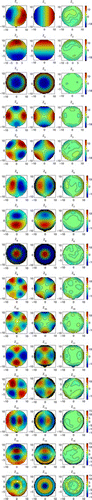
Figure 13 RMS error for the Zernike mode shapes experimentally generated using the MFDM. (Figure is provided in color online.).

5. CONCLUSIONS

A decentralized robust PID controller design method is proposed for the shape control of the magnetic fluid mirror. First, a three-step procedure is used to generate an approximate dynamic decoupled model of the plant representing mainly the wavefront corrector and the sensor. Based on the decoupled model, a robust PID controller is then developed to make the closed loop system robustly stable in the face of modeling errors, while providing optimal tracking performance. The decentralized controller gains are determined by iteratively solving properly formulated linear matrix inequalities. The designed PID controller is then successfully evaluated on an experimental adaptive optic system comprising a 19 channels prototype magnetic fluid deformable mirror.

APPENDIX

In this appendix, an algorithm is proposed to solve for the PID controller gains. First, using Schur complement, inequality (19) can be written as

which is equivalent to Cao et al. (1998)

Since , then we have

Then a sufficient condition for (A2) to be satisfied can be obtained with α ≤0 as

Let . Then (A3) is equivalent to

Similarly, a sufficient condition for (20) can be obtained as

where . In the following, an iterative LMI algorithm will be used to obtain a sub-optimal solution for the optimization problem OP1. A similar algorithm has been used in Cao et al. (1998) to solve a static output feedback stability problem. The main idea behind the following algorithm is to first find a set of gains F such that the robust stability condition (20) is satisfied, and then to further search within this set of gains for a solution that minimizes the H ₂ performance.

Algorithm

Step 1: Select , Q > 0, and solve for and P > 0 from the following algebraic Riccati equation:

Set i = 1, , X _i  = P and an initial H ₂ performance value γ₂. Let and .

Step 2: Minimize α _i subject to the following LMI constraints for unknown , P _i  > 0, F and α _i

Step 3: If α _i  ≤ 0, let , , and , then go to step 5.

Step 4: If |a _i−1 − a _i | < δ, a prescribed tolerance, the optimal problem OP1 may not be solved by F or try different and Q in step 1 and run the algorithm again. Otherwise, minimize subject to (A5), (A6) and (A7) for the unknowns , P _i and F. Set i = i + 1, and X _i  = P _i−1, then go to step 2.

Step 5: Solve min β _i subject to (A5), (A6) and (A7) for unknown , P _i , and F. If |β _i−1 − β _i | < ϵ, a prescribed tolerance, stop.

Step 6: Minimize trace(P _i ) subject to (A5), (A6) and (A7) for the unknowns P _i and F. Set i = i + 1, and X _i  = P _i−1, then go to step 5.

REFERENCES

- Baudouin , L. , C. Prieur , F. Guignard , and D. Arzelier . 2008 . Robust control of a bimorph mirror for adaptive optics systems . App. Opt. 47 ( 20 ): 3637 – 3645 .
- Borra , E. F. , D. Brousseau , and A. Vincent . 2006 . Large magnetic liquid mirrors . Astron. Astrophys. 446 ( 1 ): 389 – 393 .
- Brousseau , D. , E. F. Borra , H. J. Ruel , and J. Parent . 2006. A magnetic liquid deformable mirror for high stroke and low order axially symmetrical aberrations. Opt. Exp. 14(24):11486–11493.
- Cao , Y. , J. Lam , and Y. Sun . 1998 . Static output feedback stabilization: An ILMI approach . Automatica 34 ( 12 ): 1641 – 1645 .
- Doble , N. and D. T. Miller . 2006 . Wavefront correctors for vision science . In Adaptive Optics for Vision Science: Principles, Practices, Design and Applications . eds. J. Porter , H. Queener , J. Lin , K. Thorn , and A. Awwal . Hoboken , NJ : John Wiley & Sons .
- Hampson , K. M. 2008 . Adaptive optics and vision . J. Mod. Opt. 55 ( 21 ): 3425 – 3467 .
- Hardy , J. W. 1998 . Adaptive Optics for Astronomical Telescopes . New York : Oxford University Press .
- Iqbal , A. and F. Ben Amara . 2008 . Modeling and experimental evaluation of a circular magnetic-fluid deformable mirror . International Journal of Optomechatronics 2 ( 2 ): 126 – 143 .
- Iqbal , A. , Z. Wu , and F. Ben Amara . 2009 . Closed-loop control of magnetic fluid deformable mirrors . Opt. Exp. 17 ( 21 ): 18957 – 18970 .
- Iqbal , A. , Z. Wu , and F. Ben Amara . 2010 . Mixed sensitivity H ∞ control of magnetic fluid deformable mirrors . IEEE/ASME Transactions on Mechatronics 15 ( 4 ): 548 – 556 .
- Laird , P. , E. F. Borra , R. Bergamesco , J. Gingras , L. Truong , and A. Ritcey . 2004 . Deformable mirrors based on magnetic liquids . SPIE Advancements in Adaptive Optics Conf. Proc. 5490 : 1493 – 1501 .
- Pruss , C. and H. J. Tiziani . 2004 . Dynamic null lens for aspheric testing using a membrane mirror . Opt. Commun. 233 ( 1–3 ): 15 – 19 .
- Scherer , R. C. , P. Gahinet , and M. Chilali . 1997 . Multiobjective output-feedback control via LMI optimization . IEEE Transactions on Automatic Control 42 ( 7 ): 896 – 911 .
- Skogestad , S. and I. Postlethwaite . 2004 . Multivariable Feedback Control: Analysis and Design . West Sussex , England : John Wiley & Sons .
- Tyson , R. K. 2000 . Introduction to Adaptive Optics . Bellingham , WA : SPIE Press .
- Zhou , K. , J. C. Doyle , and K. Glover . 1995 . Robust and Optimal Control . Upper Saddle River , NJ : Prentice Hall .