Probabilistic Tracking Method Based on the Spatial Bin-Ratio Information

Abstract

We proposed a new similarity measure method which could be used within the framework of probability trackers based on the particle filter to track the object. In the particle filter framework, the state transition model is chosen as the simple second-order auto-regressive mode, and the state measure is chosen as the BBRS (Blocks-Bin-Ratio-Similarity). The BBRS considers both the spatial information and the ratios between bin values of histograms. The simulation experiment was made to compare with the similarity measures based on color-histogram and the Bin-Ratio Similarity, and the tracking results in the videos showed that the BBRS-based similarity measure was more discriminative than the color histogram similarity measure in robustly tracking the object in challenging videos where the appearance and motion are drastically changing over time.

Keywords:

• BBRS
• color histogram
• particle filters
• similarity measure
• visual tracking

NOMENCLATURE

B	=	number of the histogram
BBRS	=	BBRSc distance between the reference histogram q with c3 bins and the candidate histogram p with c3 bins (c = 4, 8, 16)
chr	=	reference histogram
chc	=	candidate histogram
dist	=	BRD distance between the reference histogram and the candidate histogram
d	=	BBRS distance between the reference histogram and the candidate histogram
dk	=	distance corresponding to the k-th particle (k = 1,2 … 50)
N	=	number of the particles
Ne	=	number of effective bins between the reference histogram and the candidate histogram
p	=	set of B candidate histograms
p b	=	histogram of the b-th candidate block (b = 1,2,3,4)
q	=	set of B reference histograms
q b	=	histogram of the b-th reference block (b = 1,2,3,4)
Xt	=	state vector of the system at time t
	=	current estimation state of the object at time t
Yt	=	observation value at time t
Y 1:t	=	set of all observation value up to time t
Greek Letters	=
	=	weight of the k-th particle (k = 1,2, … 50)
λ b	=	weight associated to the b-th block (b = 1,2,3,4)
σ	=	control parameter of the likelihood function

1. INTRODUCTION

Histograms have been proved to be a powerful representation for an image and widely applied to visual tracking. So far a large number of tracking algorithms, which roughly comprise of deterministic methods and stochastic methods, have been proposed to achieve the desired results in real-world scenarios (Iosifidis et al. 2011; Lazaros et al. 2008). Among various deterministic methods (Comaniciu et al. 2003; Yilmaz et al. 2006; Wang et al. 2010; Leichter et al. 2010), the kernel tracking (Comaniciu et al. 2003) method used the mean shift algorithm for tracking and is very successful. However, these methods are sensitive to background clutter, occlusions, and quick moving objects. Particle filters (Isard and Blake 1998) are significant methods among various stochastic methods (Isard et al. 1998; Wang et al. 2007; Birchfield and Rangarajan 2007; Ross et al. 2008; Kristan et al. 2009; Kwon et al. 2010; Cheng and Hwang 2009; Wu et al. 2010) and effective methods for nonlinear and non-Gaussian estimate state estimation. Meanwhile, particle filters are rather simple, robust and effective. The similarity measure is very important to the result of particle filters because the weights of particles are proportional to the similarity measure, and the sampling of particles relies on the similarity measure.

Due to the discarding of all spatial information of the object, the color-histogram based similarity measure has greatly affected the performance of both deterministic and stochastic methods in realistic videos including pose variation and severe occlusion (Wang et al. 2007). To address this issue, a lot of researchers have put efforts into this problem (Wang et al. 2010; Birchfield and Rangarajan 2007; Adam et al. 2006; Xie et al. 2010). The spatiograms (Birchfield and Rangarajan 2007) are histograms with the spatial means and covariance of the pixels to capture the spatial information of the object, and it has been used for particle filter tracking, head tracking, and image and video retrieval (Birchfield and Rangarajan 2007; Ulges et al. 2006). In order to solve occlusion, Adam et al. (2006) introduced a fragment-based tracking method that combined spatial information. Wang et al. (2010) proposed a fragment-based method which fused multiple spatially distributed fragments. Recently, the Bin-Ratio dissimilarity (BRD) (Xie et al. 2010) using the ratios between bin values of histograms has been successfully used in the category and scene classification, but it neglected all the spatial information of the object.

Motivated by the fragment-based tracking method (Adam et al. 2006) and BRD (Xie et al. 2010), we propose a new similarity measure BBRS to improve the discrimination of particle filters. BBRS considers both the ratios between bin values of histogram and the spatial information of the object. So it is more robust to noise than the color-histogram based Bhattacharyya measure. Compared with other popular methods, our method can robustly track the object in many challenging scenes including clutter, severe occlusions, pose variations, and illumination changes. The rest of the article is organized as follows. Section 2 gives a brief overview of the particle filters. Section 3 describes the proposed similarity measure BBRS. Our experimental results and comparisons are presented in Section 4. Finally, our conclusion and future directions are given in Section 5.

2. The Brief Introduction of Particle Filters

Particle filters, also called Bootstrap filtering (Gordon et al. 1993) or condensation (Isard and Blake 1998), are effective methods for nonlinear and non-Gaussian state estimation. In the general case, assume X _t  = [x y s] a state of the system at time t, where x, y, s denotes the x, y position and scale of the object, respectively. Meanwhile, let Y _t denote the observation at time t, and Y _1:t denote a set of all observation up to time t. Assuming that the state of the system is a first-order Markov p(X _t |X _1:t − 1) = p(X _t |X _1:t − 1), and the measures Y are independent each other, and the propagation with the dynamic process is that it can be expressed by equations (1) and (2).

During tracking, the formulation of the tracking problem is to maximize the posterior probability p(X _t |Y _1:t ), which is proportional to

where, p(X _t |X _t − 1) denotes the state transition model that predicts the current state X _t given the previous state X _t−1 , and p(Y _t |X _t ) represents the observation likelihood of the current state X _t , in other words, it denotes the probability distribution of visual features.

Given the state transition model p(X _t |X _t − 1), the previous posterior probability p(X _t |Y _1:t-1 ), the observation model p(Y _t |X _t ) and the current posterior probability of the particle filters can be approximated by a set of weighted particles which are updated by recursive method, where k ∈ [1,N], N is the number of the particles. In this article, the weight of the particles is defined by equation (4).

where, represents observation of the probability from the k-th particle, hence the current state of the object can be obtained by the minimum mean square error (MMSE) estimate over the posterior probability p(X _t |Y _1:t )

For the details of particle filter, refer to Gorden et al. 1993.

3. TRACKING METHOD BASED ON BBRS

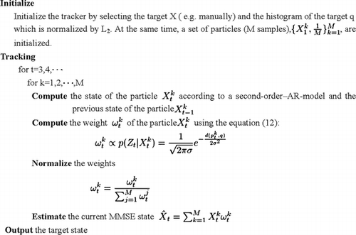
In this section, we define the similarity measure based on the BBRS for the particle filters. We start by reviewing the basic concepts for Bin-Ratio dissimilarity (Xie et al. 2010), then we define the similarity measure based on BBRS, the demonstration of discriminative power is discussed in Section 3.3. Section 3.4 describes the complexity of BBRS. Finally we give the complete algorithm pseudo code in Section 3.5.

3.1. Bin-Ratio Dissimilarity

Let us assume ch _r is a reference histogram of an image, which is computed by the kernel method in (Comaniciu et al. 2003), and ch _c denotes the candidate histogram of the image at time t, which is also computed by the kernel method in (Comaniciu et al. 2003). At the same time, we also need to assume that both histograms are also normalized by L ₂ norm. Let represent the dissimilarity between the i-th bin of ch _r and the i-th bin of ch _c and be expressed as equation (6).

Therefore, the bin-ratio dissimilarity dist (ch _c , ch _r ) between ch _c and ch_r can be defined as equation (7).

3.2. Blocks-Bin-Ratio Similarity

The bin-ratio dissimilarity neglects any spatial information of the object, and it is bound to affect the identification, because it only considers the ratios between bin values of histograms. In order to further improve the performance of identification, based on modified BRD, we propose a new similarity BBRS that considers both the spatial information and the ratios between bin values of histograms. Firstly, the reference object and candidate object are divided into several blocks respectively. Then we compute the histogram of each block and BRS (Bin-Ratio-Similarity) value corresponding to each block pair. Finally, BBRS are computed by the BRS value of each block.

Let us describe the reference object by a set of B histograms, the configuration expressed by the q = [q ₁ … q _b  … q _B ]. Assume the candidate object is the same size as the reference object, and described by a set of B histograms p = [p ₁ … p _b  … p _B ], where q _b , p _b denotes the histogram of the b-th block respectively, which are normalized by L ₂ norm. In this article, L ₂ norm can be defined by equation (8).

In order to compute the similarity measure of the two histograms p _b and q _b , the similarity measure d(p _b , q _b ) is defined by equation (9).

where, U is the total number of bins and N _e is the number of bins and each pair of bins has at least one non-zero value in the two histograms p _b , q _b . Consequently, we define the blocks-bin-ratio similarity d (p, q) between the reference histogram q and the candidate histogram p as

where λ _b represents the weight associated to the b-th block which is defined as

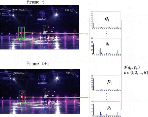
The new similarity BBRS is computed as follows. First, the tracked object from the video sequence is simply equally divided into four rectangular blocks. Then, the histogram of each block is computed and the similarity d(p _b , q _b ) between the normalized q _b , and p _b using L2 is calculated by (9). Finally, the similarity d(p, q) is expressed as equation (10), as shown in Figure 1. By the similarity measure of BBRS, the observation likelihood may be represented as

where σ is a control parameter and d _k (p, q) is the similarity measure corresponding to the k-th particle. As can be seen from equation (12), the observation likelihood varies directly with the similarity measure d _k (p, q) and inversely with the control parameter σ. After the σ is fixed, the observation likelihood is directly related to the d _k (p, q), in other words, the weight of the k-th particle is also directly related to the d _k (p, q), hence, the bigger the similarity measure is, the more reliable sample is. According to equations (5) and (12), the current state can be given as

From equation (13), we can see that the discriminative ability of the similarity measure is very important because it can affect the accuracy of the state. Therefore, it is very necessary to design the strong discriminative ability of the similarity measure, the strong discriminative ability of our similarity measure is shown in Section 3.3.

Figure 1 Computational process of the BBRS of the tracked object from both the t-th frame and the (t + l)-th frame. The green box contains the tracked object that is simply equally divided into four rectangular blocks using two red lines, q _b , and p _b denote the histogram with 64 bins of the b-th blocks, and d(q _b , p _b ) denotes the BBRS similarity demonstrated by equation (9), in which q _b , and p _b are normalized by the L2 norm (color figure available online).

3.3. Demonstration of Discriminability

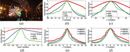
In order to test the proposed similarity measure discriminative ability, we compare our method with three other kinds of similarity measures including color-histogram, BRS, and BBRS as well as the influence of bin values in BBRS on the results. BBRSc represents BBRS between the object histogram q with c ³ bins and the candidate histogram p with c ³ bins, where c is 4, 8 and 16, respectively, and q, p satisfies (in RGB color space, each channel is quantified into 8 levels). As can be seen from Figure 2 b–d, the proposed similarity measure is more discriminative than the other similarity measures. This is mainly due to the fact that we consider not only the ratios between bin values of histograms but also spatial information of the object. In Figure 2 e–f, even though we only take the histogram with a total of 64 bins, the BBRS similarity is more discriminative than Bhattacharyya similarity with a total of 4096 bins. And it is also noted that the new similarity becomes relatively more discriminative when we increase the number of bins, however the difference between the similarity measures is rather slight.

Figure 2 The scores by three kinds of similarity measures based on color-histogram, BRD and BBRS, and by the BBRS-based similarity measure with different bin values. (a) We select a face as the referent object model. From (b) to (d), the results are the scores by different similarity measures over (b) x-translation (in pixels), (c) y-translation (in pixels), and (d) scale (the ratio to the size of target). (e–f) are the scores based on the BBRS similarity measure with different bin values over (e) x-translation and (f) y-translation. The BBRS4 is the BBRS with 64 bins, the BBRS8 is the BBRS with 512 bins and the BBRS16 is the BBRS with 4096 bins (color figure available online).

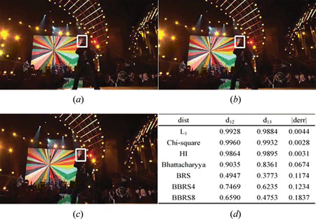
To further compare the discriminative ability of different similarities including L₁, Chi-square, Histogram Intersection (Swain and Ballard 1991), Bhattacharyya, BRS with 16³ bins, respectively, BBRS4 and BBRS8, we calculate similarities between Figures 3a, 3b, and 3c using these methods. In Figure 3, three images are consecutive three frames in singer sequences, Figure 3 d shows the values of different similarity measures and the differences between them. Meanwhile, we can still see that the difference of the proposed similarity measure is bigger than that of the other similarity measures from Figure 3 d, that is to say, the proposed similarity measure is more discriminative than the other similarity.

Figure 3 Results of several similarity measures in three selected object. (a), (b) and (c) are three consecutive frames which contain the tracked object, and (d) shows similarities between the selected face from (a), (b), and (c) computed by several different methods, in which L1, Chi-square, and HI indicates L1 distance, Chi-square distance and Histogram Intersection distance, respectively, and derr is computed by derr = |d12-d13| (color figure available online).

3.4. Computational Complexity

To compare the computational complexity of the proposed method and the basic particle filter, we firstly compare the computation complexity of the BBRS with that of the Bhattacharyya. The computation complexity of the BBRS is O(blocks × N ₁) when the number of bins of color histogram is N ₁, and that of the Bhattacharyya measure is O (N) when the number of bins is N of color histogram, generally speaking, N is set to 4096 in order to obtain the better performance. As shown in Figure 2, the BBRS with 64 bins is better than the Bhattacharyya with 4096 bins, so the BBRS is remarkable lower than the Bhattacharyya when N ₁ is 64 and the block number is 4, even if N ₁ is equal to 512, our similarity is still better than the Bhattacharyya. Hence the complexity of our method with 512 bins is lower than that of the basic particle filter with 4096 bins under the same condition of the experiments.

3.5. The Complete Algorithm

We have discussed the most important ingredient for a robust BBRS tracker. Now, we give the pseudo-code for our method in Figure 4.

Figure 4 The complete tracking algorithm of BBRS.

4. EXPERIMENTS

To test the effectiveness of the similarity measure based on BBRS, we make six sequences by the video sequences available ¹ . In all experiments, a reference target is manually selected in the initial frame and is divided into 4 blocks for the BBRS tracker. The color space used is RGB space, and quantified 8 bins for each color channel. The scale which may produce the maximum score is selected when scale changes are bound to ±10% in each video frame (Comaniciu et al. 2003).The number of the particles is set to 50. All the experiments are carried out with a core 4 Duo 2.9 GHz processor with 2 GB RAM under Matlab2009a.

In Section 4.1., we compare the results of four tracking methods including our method,VTD (visual tracking decomposition) (Kwon et al. 2010),the spatiogram method (Birchfield and Rangarajan 2007), and the conventional particle filter (Gordon et al. 1993) in occlusion and pose variation scenery. In Section 4.2., we show the performance of our method, BRS based method, the spatiogram and VTD method in pose variation, and severe occlusion or illumination change. In Section 4.3., we discuss the tracking methods based on the BBRS with different bins in the complete occlusion scenery. We demonstrate the results of the proposed method, VTD, the spatiogram method, and the conventional mean shift (Comaniciu et al. 2003) in Section 4.4. Finally the results of the proposed method and multiple reference color histograms tracking method (MRCHT) is discussed in Section 4.5.

4.1. Comparing Results in Occlusion and Pose Variation Scenery

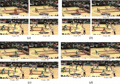
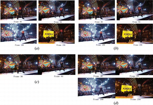
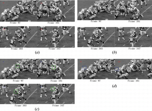
We show the performances of the four trackers in the face of a second-order-AR model, pose variation and severe occlusion. From Figures 5-8, we can see that the proposed method outperforms other methods including the conventional particle filter (Gordon et al. 1993), the spatiogram tracking, and the VTD method when the target is severely occluded and pose variance. In Figures 5-8 a, our method can robustly track the target in soccer, skating, basketball, and motinas-toni-change-ill sequences because of the fact that our method considers both the ratios between bin values of histograms and spatial information of the object. Our method can effectively solve these pose variations and severe occlusion. Meanwhile, the VTD method can also successfully track the object in these challenge sequences. But its computational complexity is very high, so it takes 1–5 seconds per frame. On the contrary, other methods either are severely drifted or track the wrong object when these pose variation or severe occlusion occur as shown in Figures 5-8 b–c object.

Figure 5 Tracking results of the methods including (a) proposed method, (b) the conventional particle filter, (c) the spatiogram method, and (d) the VTD method in a soccer sequence when there is severe occlusion (color figure available online).

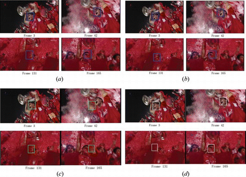
Figure 6 Tracking results of the methods including (a) our method, (b) the conventional particle filter, (c) the spatiogram method, and (d) the VTD method in a skating sequence when there is severe occlusion and pose variation (color figure available online).

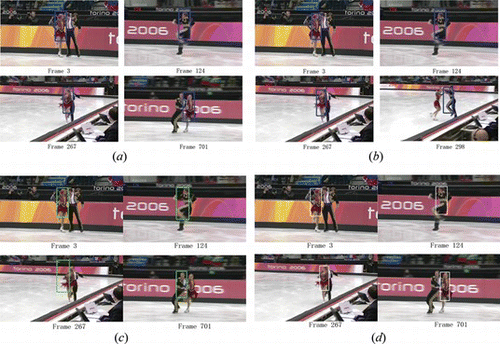
Figure 7 Tracking results of the methods including (a) our method, (b) the conventional particle filter, (c) the spatiogram method, and (d) the VTD method in a basketball sequence when there is severe occlusion and pose variation (color figure available online).

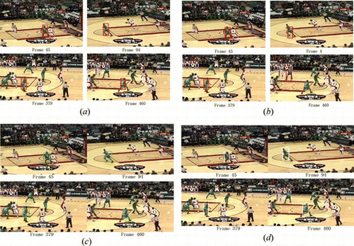
Figure 8 Tracking results of the methods including (a) our method, (b) the conventional particle filter, (c) the spatiogram method, and (d) the conventional mean shift method in a motinas-toni-change-ill sequence when there is complete occlusion (color figure available online).

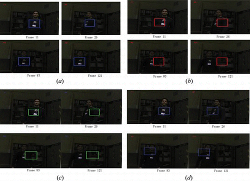
The relative ability of both methods to deal with pose variation is depicted in Figures 6, 7. Two skaters have different pose variation throughout the sequence. Our method and the VTD achieve the most accurate tracking results. On the contrary, the conventional particle filter and the spatiogram method achieve less accurate tracking. When the object is severely occluded by other objects in Figures 5-8, we note that our method achieves the better performance in tracking. Especially, when the object is completely occluded for a long time in Figure 8, our method may still track the object. On the contrary, the object tracked by other methods drifts slowly until it is lost over time, as depicted in Figure 8 b–d.

4.2. Comparing Results in Illumination Change and Pose Variation Scenery

Figures 9 and 10 demonstrate how our method outperforms the tracking algorithm based on the BRS, the spatiogram method, and the VTD method when the pose of the object is changed severely and the illumination is changed drastically. In Figures 9 and 10, our method the VTD method, and the tracking algorithm based on the BRS can also robustly track the object. Our method and the VTD method achieve the better accurate tracking results. However the spatiogram method fails to track the object in Figure 10 c.

Figure 9 Tracking results of the methods including (a) our method, (b) the conventional particle filter, (c) the spatiogram method, and (d) the VTD method in a basketball sequence when there is severe occlusion and pose variation (color figure available online).

Figure 10 Tracking results of the methods including (a) our method, (b) the conventional particle filter, (c) the spatiogram method, and (d) the VTD method in a singer sequence when there is severe illumination change (color figure available online).

4.3. Comparing the Proposed Method Between 64 Bins and 512 Bins

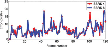
The tracking method based on the BBRS with the total 512 bins outperforms the method based on the BBRS with the total 64 bins, but both methods can robustly track the object and the difference is slight between the two methods, as shown in Figure 11.

Figure 11 Tracking results over a long time with complete occlusion (color figure available online).

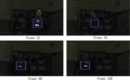
Figure 12 displays the performance of both methods in the motinas_toni_change_ill sequence. The ground truth is labeled by hand. The red line represents the method based on the BBRS with the total 512 bins and the blue represents the method based on the 64 bins.

Figure 12 Tracking error in pixels using the BBRS4 (red) versus BBRS8 (blue) in a motinas_toni_change_ill seq (color figure available online).

4.4. Comparison Results in A Football Scenery

In Figure 13 a–b, our method and the VTD method can also robustly track the sportsman wearing a helmet in a football sequence under severe background clutter. Especially, when two sportsman wearing a similar helmet collided with each other at frame 303 and 347, two methods can still robust track the player, However, the spatiogram method and the conventional mean shift method (Comaniciu et al. 2003) also fail to track the player, especially, when two sportsman wearing a similar helmet collided with each other.

Figure 13 Tracking results of (a) our method, (b) the conventional mean shift, (c) the spatiogram method, and (d) the VTD method in a football sequence when there is severe background clutter. Note that (a) and (d) can also robustly track the object (color figure available online).

The tracking time of per frame is significantly different, the processing time of the conventional mean shift method is the shortest one which takes 0.01 second, and the spending time of the visual tracking decomposition method is the longest, which takes 1.5 seconds. However, the spending time of our method takes only 0.03 second.

4.5. Comparision Results in Switching Between Color and IR Scenery

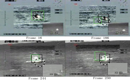
We tested a boat sequence that includes switching between color and IR (infrared) modes, as is illustrated in Figure 14. Our method can robustly track the object whether in the color modes or IR modes, and we obtain better performance of tracking, on the contrary, although multiple reference color histograms tracking can also track the object, the performance of tracking is poor, and the results of MRCHT are far away the true position of the object, as shown in frame 186, 244 and 250. The spatiogram tracker can track the object, however the performance is the poorest, and is especially prone to being affected by the background clutter, as shown in frame 186.

Figure 14 Comparison results of the proposed method, the spatiogram method, and the MRCHT method (Leichter et al. 2010). Note that the black box shows the results of our method, and the black and white circle shows the results of MRCHT, and the green box shows the results of the spatiogram method (color figure available online).

5. CONCLUSION

We have presented an effective particle filtering framework for tracking by Blocks-Bin-Ratio-Similarity (BBRS). The similarity measure considers both the spatial information and the ratios between bin values of histograms. Hence, the BBRS is more discriminative than the Bhattacharyya similarity measure and the BRS. The particle filter based on BBRS, which takes a small number of particle and the color histograms with a few of bins, can robustly track the object under different challenge videos that comprising sever background clutter, pose variation, severe occlusion and illumination change. In spite of increasing the number of the particles and the bins of color histogram, the performance becomes better and more consistent than that of the small number particles and bins. However it takes more time to compute the BBRS. Moreover the number of the blocks of the BBRS is also vital for visual tracking, the more it is, the better its performance is, but it also takes more time to compute the BBRS. Although the proposed BBRS measure shows its competence over some existing measure, it should be noticed that it easily fails to track the object with large scale, similarity of color, and occlusion over a very long time.

Compare among the conventional particle filter tracking, VTD, spatiogram, and MRCHT algorithm, the proposed method outperforms other methods in challenging environments, and the tracking performance approximates VTD, but its speed is faster than that of the VTD. In future work, we plan to extend the BBRS-based similarity for other tracking methods, such as mean shift tracking, and we will fuse other features to track very similar objects in scenes.

ACKNOWLEDGMENTS

We would like to thank the editor in chief Professor Hyungsuck Cho and the reviewers for their valuable comments during the review process, which improved the article. Research work was partially supported by the Chinese National Science Foundation (NSFC Grant No. 60903142), the Natural Science Foundation of CQ-CSTC (CSTC 2009BB3192).

Notes

¹ http://cv.snu.ac.kr/research/~vtd and http://www.eecs.qmul.ac.uk/~andrea/spevi.html.

REFERENCES

- Adam , Amit , Ehud Rivlin , and Ilan Shimshoni . 2006 . Robust fragments-based tracking using the integral histogram. Proceedings of IEEE Conference on Computer Vision and Pattern Recognition 798–805 .
- Birchfield , S. T. and S. Rangarajan . 2007 . Spatial histograms for region-based tracking . Electronics and Telecommunications Research Institute 29 ( 5 ): 697 – 699 .
- Comaniciu , D. , V. Ramesh , and P. Meer . 2003 . Kernel-based object tracking . IEEE Transactions on Pattern Analysis and Machine Intelligence 25 ( 5 ): 564 – 577 .
- Cheng , H. and J. Hwang . 2009 . Adaptive particle sampling and adaptive appearance for multiple video object tracking . Signal Processing 89 ( 9 ): 1844 – 1849 .
- Gordon , N. J. , D. J. Salmond , and A. Smith . 1993 . Novel-approach to nonlinear non-Gaussian Bayesian state estimation . IEE Proceedings-F Radar and Signal Processing 140 ( 2 ): 107 – 113 .
- Iosifidis , A. , Spyridon G. Mouroutsos , and Antonios Gasteratos . 2011 . A hybrid static/active video surveillance system . International Journal of Optomechatronics 5 ( 1 ): 80 – 95 .
- Isard , M. and A. Blake . 1998 . CONDENSATION – conditional density propagation for visual tracking . International Journal of Computer Vision 29 ( 1 ): 5 – 28 .
- Kristan , M. , J. Pers , S. Kovacic , and A. Leonardis . 2009 . A local-motion-based probabilistic model for visual tracking . Pattern Recognition 42 ( 9 ): 2160 – 2168 .
- Kwon , Junseok and Kyoung Mu Lee . 2010 . Visual tracking decomposition. Proceedings of IEEE Computer Society Conference on Computer Vision and Pattern Recognition 1269–1276 .
- Lazaros , N. , G. C. Sirakoulis , and A. Gasteratos . 2008 . Review of stereo vision algorithms: From software to hardware . International Journal of Optomechatronics 2 ( 4 ): 435 – 462 .
- Leichter , I. , M. Lindenbaum , and E. Rivlin . 2010 . Mean shift tracking with multiple reference color histograms . Computer Vision and Image Understanding 114 ( 3 ): 400 – 408 .
- Ross , D. A. , J. Lim , R. S. Lin , and M. H. Yang . 2008 . Incremental learning for robust visual tracking . International Journal of Computer Vision 77 ( 1–3 ): 125 – 141 .
- Swain , M. and D. Ballard . 1991 . Color indexing . International Journal of Computer Vision 7 ( 1 ): 11 – 32 .
- Ulges , Adrian , Christoph Lampert , and Daniel Keysers . 2006 . Spatiogram-based shot distances for video retrieval. Proceedings of TRECVID Workshop 1–10 .
- Wang , Fanglin , Shengyang Yu , and Jie Yanga . 2010 . Robust and efficient fragments-based tracking using mean shift . AEU-International Journal of Electronics and Communications 64 ( 7 ): 614 – 623 .
- Wang , H. Z. , D. Suter , K. Schindler , and C. H. Shen . 2007 . Adaptive object tracking based on an effective appearance filter . IEEE Transactions on Pattern Analysis and Machine Intelligence 29 ( 9 ): 1661 – 1667 .
- Wu , M. , X. Peng , Q. Zhang , and R. Zhao . 2010 . Patches-based Markov random field model for multiple object tracking under occlusion . Signal Processing 90 ( 5 ): 1518 – 1529 .
- Xie , N. , H. Ling , W. Hu , and X. Zhang . 2010. Use bin-ratio information for category and scene classification. Proceedings of IEEE Computer Society Conference on Computer Vision and Pattern Recognition 2313–2319.
- Yilmaz , A. , O. Javed , and M. Shah . 2006 . Object tracking: A survey . ACM Computing Surveys 38 ( 4 ): 45 .