Methods for Optical Shape Measurement and their Measurement Uncertainty

Abstract

There is a wide spectrum of optical 3-D sensors based on only a few basic principles. We calculate the measurement uncertainty for several “paradigm” methods, by means of the Cramér-Rao lower bound. It turns out that when all other sources of noise are neglected, the shot noise becomes the ultimate limit of the measurement uncertainty and the measurement uncertainty can be traced back to a Heisenberg uncertainty product. Consequently, making one of the factors uncertain, the other factor will become more precise. The different methods vary only by the way how this “uncertainty” is generated.

Keywords:

• coherence noise
• measurement uncertainty
• shape measurement
• shot noise
• uncertainty relation

NOMENCLATURE

a	=	Parameter
C	=	Constant
D 0	=	Waist diameter of the laser beam
ħ	=	Reduced Planck constant
I	=	Intensity
I 0	=	Intensity of the light source
k	=	Wave number
k	=	Wave vector
k 0	=	Wave number of the light source
k x , k y	=	Lateral components of wave vector
k z	=	Longitudinal component of wave vector
l	=	Distance between the CCD camera and the surface
L	=	Measurement range
N	=	Number of photons
NA	=	Numerical aperture of the objective lens
p	=	Momentum
p z	=	z-component of momentum
R	=	Radius of the laser beam
S	=	Spectral density
u	=	Observation aperture of the lens
x, y	=	Lateral coordinates
z	=	Depth coordinate
α	=	Tilt angle
δX	=	Lateral resolution
Θ	=	Triangulation angle
λ0	=	Wavelength of the light source
ϕ	=	Phase change

1. INTRODUCTION

We will discuss the ultimate limit of the statistical measurement uncertainty of several “paradigm” measurement methods. We refer to some earlier papers.^[ 1-5 ^] A summary is given in.^{[ 6 ]} The earlier discussion was oriented towards the physics and the information theory of these limits; here we will exploit a statistical tool, the “Cramér-Rao lower bound”.^{[ 7 ]} There are various methods for optical shape measurement. Some of them are suitable for the measurement of optically smooth surfaces, the paradigms are classical interferometry and phase measuring deflectometry.^{[ 2 , 4 ,} 8-10 ^] Optically rough surfaces are commonly measured by triangulation with a multitude of implementations, among them laser triangulation and the so called “fringe projection,” but as well focus search like confocal microscopy. Only few methods are able to measure optically smooth and optically rough surfaces. The paradigm is white-light interferometry (WLI).^{[ 11 ]}

Note that a surface is regarded as optically rough for a specific instrument when the height variations of the surface within the resolution cell of the imaging system exceed one-fourth of the wavelength of the light. The deep consequence is that the attribute smooth or rough does not only depend on the geometrical roughness parameters of the surface but as well on the observation aperture (and the wavelength). So we find that the observer is strongly involved.

We will further find (not surprisingly) that the illumination plays a big role. The Rayleigh criterion for the diffraction limited telescope resolution needs only the aperture diameter. But if noise comes into play, the source, the receiver and energy are important, as already Ronchi stated.^{[ 12 ]} We may add that the coherence (spatial, and a little bit less important temporal coherence) plays a major role.^{[ 13 ]} We will take into account these parameters and discuss the limit of the statistical measurement uncertainty and its dependence on the important features of various methods.

2. STATISTICAL MEASUREMENT UNCERTAINTY

We cannot measure the shape of objects arbitrarily precise because of the ubiquitous noise. According to the Guide of Uncertainty of Measurement^{[ 14 ]} or DIN 1319,^{[ 15 ]} the measurement uncertainty is a parameter that characterizes the dispersion of the measured values. The parameter may be, for example, a standard deviation. A measurement has imperfection that give rise to an error. Traditionally, an error is viewed as having two components, a random component and a systematic component. When systematic errors (e.g., by geometrical distortion) are not considered, the statistical contributions of the light result in an uncertainty contribution that is investigated in our paper.

Diffraction is one further source of measuring uncertainty. However, many 3-D measuring principles are based on the localization (and not that much on the resolution) of an optical signal. As well known, the localization uncertainty can be much better than the diffraction limited resolution, provided the sampling theorem is not at all violated.

A suitable and quite general tool to determine the measurement uncertainty of optical shape measurement methods is the Cramér-Rao lower bound.^{[ 16 ]} In order to apply the Cramér-Rao lower bound, we need to know only the analytical expression of the signal and the probability density function of the noise.

In the daily life of an opticist, it is very important to know about the dominant source of noise. The major sources are: the random arrival of photons at the detector (shot noise) and coherent noise. These are fundamental, although it may happen that the positioning noise of translation stages, or quantization noise of the A/D conversion become dominant.

Shot noise holds a unique position. Shot noise is a fundamental property of the quantum nature of light and cannot be, even theoretically, reduced. Shot noise imposes a basic limit on the minimum measurement uncertainty that can be achieved, after all other sources are “avoided.” So in what follows we will only consider shot noise, unless we have to deal with the much larger coherent noise.

Laser light is described by a Poisson photocount distribution. Thermal light obeys Mandel-Rice photocount distribution. However, when the integration time of the detector is much higher than the coherence time of the used light, the MandelRice distribution turns into Poisson distribution.^{[ 17 ]} Then the variance of the photocounts (ΔN)² is equal to the number N of photocounts. For large N, the Poisson distribution approaches the normal distribution with mean N and variance N. Therefore we can assume that the probability density function of the noise is Gaussian with zero mean and variance N for common light sources like laser or incandescent lamps and LEDs.

Let us assume that the analytical expression of the signal is given by

In Equation (1), I is the intensity at the detector, I ₀ is the intensity of the light source, a is the measured parameter, which can be e.g., a depth coordinate (for interferometry or confocal microscopy) or an angle (for deflectometry), and f(a) is a function that describes the dependence of the signal on the measured parameter. The number of photons that are used for the measurement is equal to

where C is a constant that converts the integrated intensity to the number of photons.

From the Cramér-Rao lower bound we obtain the lower limit δa of the measurement uncertainty of the parameter a ^{[ 16 ]}

where f' denotes the first derivative of f with respect to a. The term on the right hand side of Equation (3) is the inverse of the Fisher information.^{[ 7 ]} The results from Equations (2) and (3) coincide with the results of Falconi who derived them for the angular position being the measured parameter.^{[ 18 ]}

By the combination of Equations (2) and (3) we obtain

The meaning of Equations (1)–(4) becomes clear below, when applied to particular measurement methods.

Note: If the lower limit of the measurement uncertainty of a parameter is calculated rigorously, not only one but all parameters which describe the signal, must be taken into account. From the dependence of the signal on the parameters, the Fisher information matrix as a generalization of the Fisher information is derived. The Fisher information matrix is a quadratic matrix with the dimension equal to the number of parameters. The diagonal elements of the inverse Fisher information matrix are equal to the squares of the measurement uncertainties of the individual parameters of the signal. The method of the calculation is described in.^{[ 16 ]} On special conditions (there is one dominant source of noise), which are satisfied in the presented cases, the result of the rigorous calculation is the same as that presented in Equation (4), where only one parameter is taken into account.

3. UNCERTAINTY RELATIONS

In what follows, we will compare the obtained results with Heisenberg's uncertainty product between the position z and momentum p. This uncertainty relation states that the product of the standard deviation δz of position z and standard deviation δp _z of the momentum p _z is greater or equal than one half of the reduced Planck constant ħ: δz · δp _z  ≥ ħ/2.^{[ 19 ]} The momentum p of the photon can be expressed by means of the wave number k: p = ħk. Thus we obtain an uncertainty relation that is more useful for our purpose: δz · δk _z ≥ ½. This result is valid only for one photon. For N photons we obtain

We emphasize that the wave vector k may display variations of its magnitude (wavelength) and as well variations of its spatial components k _x , k _y , k _z .

4. INTERFEROMETRY

For classical interferometry, commonly a laser with a narrow spectrum is used. We consider a Michelson interferometer. The interferometer output is the intensity at the detector expressed as the function of the position z of the measured object. The position z is representing the parameter a from Equation (1). Mathematically, the signal is described by

where k ₀ = 2π/λ₀ is the wave number for the wavelength λ₀ of the light source and ϕ describes the phase shift at the object surface. In this case, the wave vector has only a longitudinal component. The plot of the intensity is shown in Figure 1(a).

Figure 1 (a) Output signal of classical interferometry. (b) Wave number spectrum of classical interferometry.

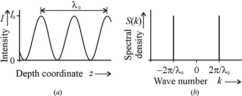
By comparison of Equations (6) and (1), one can see that f = ½(1 + cos (2k ₀ z + ϕ)). If we insert this expression into Equation (4), we obtain

In practice, the measurement is performed in a finite range L of coordinate z. This is expressed by the integration limits. We assume that the measurement range L is an integer multiple of λ₀/2. Then the measurement uncertainty is equal to

According to Equation (7), the increasing measurement range L increases the Fisher information and the number N of photons in the same way. Therefore, the measurement range L is not explicitly included in Equation (8).

The measurement uncertainty δz depends on the wavelength and the number of photons. The result described by Equation (8) is the so called standard quantum limit that follows from the uncertainty relation.^{[ 20 , 21 ]} The result given by Equation (8) differs from that presented in Equation (3) in the previous work.^{[ 22 ]} The reason is that the meaning of quantity N is different. In,^{[ 22 ]} N denotes the number of photons emitted by the light source during the measurement time. This definition is analogous to that used in.^{[ 23 ]} In Equation (8) here, N is the number of photons that are used for the measurement (it is equal to the number of detected photons if we assume the quantum efficiency of the detector to be equal to 1), that is equivalent to the definition presented in.^{[ 18 ]}

The spectral density of the signal of the classical interferometry is given by

and is illustrated in Figure 1(b). According to Equation (9), the standard deviation δk _z of the wave number is equal to

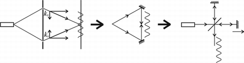
The interference of two waves in the Michelson interferometer is interpreted as the diffraction of one wave on double slit. The interpretation is illustrated in Figure 2. Both arrangements, the double-slit diffraction and the Michelson interferometer belong to a general class of double path experiments. It is apparent from Figure 2 that for the diffracted wave, it holds δk _x  = |k _x|, which is an analogous relation to Equation (10). The quantity δk _z in Equation (10) is not the spectral width of the light source (we assume a laser with a narrow spectrum as the light source).

Figure 2 The interference of two waves in Michelson interferometer interpreted as the diffraction on double slit.

By the combination of Equations (8) and (10) we obtain δk _z  · δz = 1/(2N ^1/2) that coincides with the uncertainty relation [Equation (5)].

A major disadvantage of classical interferometry is its ambiguity. This is overcome by white light interferometry (WLI).^{[ 24 , 25 ]} In WLI, a broad-band source (LED, incandescent lamp) is used. Because of the broad spectrum of the light source, the interferometer output (the “correlogram”) displays an envelope with a length of approximately the coherence length. The measurement uncertainty can be calculated by means of Equation (4). The measurement uncertainty is higher than for classical interferometry [Equation (8)] for the same wavelength and number of photons. The measurement uncertainty of WLI increases with the decreasing coherence length of the light source.

WLI can also be implemented in a manner that only the envelope is evaluated and not the phase of the correlogram. For rough surfaces, only the envelope evaluation makes sense, because the speckle phase is random.^{[ 2 ]} In this case again, the measurement uncertainty can be calculated by means of Equation (4). It turns out that now the measurement uncertainty increases linearly with the coherence length and decreases with . For rough object WLI, the shot noise is negligible, coherent noise is dominant.

For rough objects, the interferometer output encodes the local depth z(x, y) in a nonmonotonic, nonlinear (chaotic) way and the Cramér-Rao bound is difficult to estimate. But experiments and theory show that the statistical measuring uncertainty is equal to the surface roughness, independent from the lateral resolution of the optical system.^{[ 5 , 26 , 27 ]}

5. CONFOCAL MICROSCOPE

The signal of the confocal microscope is described by^{[ 28 , 29 ]}

where sinc(x) = sin(x)/x and NA is the numerical aperture of the objective lens. Here again, the position z of the object represents the parameter a in Equation (1). The signal is shown in Figure 3(a). In some references,^{[ 30 ]} the exponent of the sinc function is equal to 2 instead of 4. The exponent 2 appears also in.^{[ 22 ]} However, the magnitude of the exponent has a negligible influence on the results presented here. The measurement uncertainty calculated analogously as in the case of Equation (8), is

Figure 3 (a) Output signal of confocal microscope. (b) Wave number spectrum of confocal microscope.

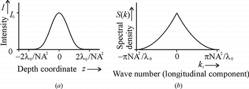
Equation (12) displays approximately the Rayleigh depth of field, for N = 1.

The spectral density corresponding to the signal described by Equation (11) has the form

In Equation (13), tri(x) denotes the triangle function. The spectrum is shown in Figure 3(b). The standard deviation δk _z of the wave number is equal to

δk _z displays the uncertainty of the longitudinal component of the k-vector (photon impulse) after passing the aperture.

By the combination of Equations (12) and (14), we obtain δk _z  · δz = 1/(2N ^1/2) which is in agreement with the uncertainty relation [Equation (5)].

6. BEAM DEFLECTION

We consider an idealized sensor to measure the angular deflection of a beam, as shown in Figure 4(a). A collimated Gaussian laser beam with the waist diameter D ₀ is focused onto a reflective flat surface. The position x of the reflected beam is detected at a CCD line target. The distance of the CCD line camera from the flat surface is equal to l. If the flat surface is tilted by an angle α, the beam is deflected by 2α and the position of the beam at the CCD line changes by x = 2lα. The output signal of such a beam deflection sensor is described by

where I ₀ is the intensity at the axis of the laser beam and R is the radius of the laser beam in the plane of the CCD line. The radius R of the beam depends on the waist diameter D ₀, the wavelength λ₀, and the distance l. For a distance l greater than the Rayleigh range of the beam, we find R = 2lλ ₀ /(πD ₀).^{[ 23 ]} Then the expression for the signal can be re-written as

Figure 4 (a) Schematic of the beam deflection sensor. (b) Schematic of triangulation.

The measurement uncertainty of the angle α is calculated by means of Equation (4)

The measurement uncertainty δα depends on the wavelength of the light, the waist diameter of the beam and the number of photons. Note that the distance l vanished! The result described by Equation (17) is identical with that of Falconi.^{[ 18 ]} For one single photon, δα displays the uncertainty after transmission of the photon through a “slit” with the width D ₀. The uncertainty of the beam angle is equal to 2δα.^{[ 22 ]}

From Equation (16), which describes the lateral distribution of the intensity of the Gaussian beam, the distribution of the lateral components k _x , k _y of the wave vector can be determined

It follows from Equation (18) that the standard deviation of k _x is equal to δk _x  = 1/R = πD ₀/(2λ₀ l). If we take into account the result of Equation (17) and that δx = 2lδα, we find that δk _x  · δx = 1/(2N ^1/2) which is in agreement with the uncertainty relation [Equation (5)].

We can consider the waist diameter D ₀ in Equation (17) as the lateral resolution distance δX at the deflecting surface. Then we obtain the uncertainty relation for the angle and the lateral coordinate^{[ 2 , 4 ]}

Equation (19) reveals an extraordinary property of deflectometry: The uncertainty product given at the left side is essentially the height uncertainty δz within the lateral resolution distance δX. It is essentially given by the wavelength divided by the SNR. It is quite easy to achieve an SNR of 500 or better, so a local height uncertainty of 1 nm can be achieved, by simple means. Deflectometry can detect extremely low height variations.

In practice, the local slope of reflecting objects is measured by phase measuring deflectometry (PMD).^{[ 2 , 4 ]} An important advantage of PMD is that it can measure the shape of the object without lateral scanning, by a few (commonly 8) exposures. In PMD, sinusoidal fringes are displayed on a monitor. The displayed fringes are observed by a CCD camera and the measured surface acts as a mirror. From the deformation of the observed fringes, the shape of the reflecting object is determined. The measurement uncertainty of PMD is up to a multiplicative factor the same as given by Equation (19).

7. LASER TRIANGULATION

Eventually, we come to the last archetype sensor principle: laser triangulation, as illustrated in Figure 4(b). From the lateral position of the scattered laser spot, the coordinate z is determined. At the first glance, there is some similarity to deflectometry, because the shape is measured via the lateral position of a narrow bright spot at a detector. However, the measuring uncertainty of triangulation is aperture dependent, while it is not for deflectometry [see Equation (19)]: the physical mechanism of the signal generation is different from deflectometry.^{[ 1 ]} Taking into account Equation (17), the expected result of the measurement uncertainty is equal to δz = λ₀/(2π sin Θ sinu N ^1/2), where u is the observation aperture of the observing lens and Θ is the triangulation angle.^{[ 1 , 18 ]}

Laser triangulation only works at rough surfaces. The rough surface destroys the wavefront of the incident light wave and the measurement uncertainty is not anymore determined by the number N of photons. Speckle noise is highly dominant,—the SNR is unity.

8. PRECISE MEASUREMENTS NEED UNCERTAINTY

The application of the uncertainty relation in Sections 4 − 6 shows that the wave number k must exhibit an uncertainty δk _z or δk _x to allow for a precise measurement of the coordinates x, respective z. The uncertainty δk can be produced in different ways, depending on the measurement method:

1.

δk is accomplished by a wide wavelength spectrum (color), as for WLI.

2.

δk originates by exploiting the spatial components of the wave vector k. If the wave vectors have various directions, their lateral components will take various values even if the absolute value of k is constant. An example where the lateral component δk x is exploited, is the beam deflection measurement: the wider the beam (δx) at the object, the smaller the angular uncertainty (δk x ). Laser triangulation: The wider the aperture of the observation (δk x ), the better is the localization (δx) of the spot image, and, hence, the distance measurement. Focus sensing: a large uncertainty of δk z allows for a small depth uncertainty δz. It should be mentioned, that k z and k x are not independent, and the big k z is achieved by a big aperture—in other words—a large δk x .

9. CONCLUSIONS

The discussion illustrates that the fundamental measurement uncertainty δz for a measured distance z can be traced back to a fundamental Heisenberg uncertainty product. This holds for classical interferometry with photon noise dominating, as well for triangulation, with speckle noise dominating. For WLI at rough surfaces, the roughness itself determines the measuring uncertainty, independently from the aperture. Deflectometry displays a similar behavior, the distance uncertainty is determined just by the photon noise, and not by the aperture of observation.

ACKNOWLEDGMENTS

We wish to thank Prof. Jan Peřina from Palacky University in Olomouc for useful suggestions during the preparation of this article.

REFERENCES

- Dorsch , R. ; Häusler , G. ; Herrmann , J.M. Laser triangulation: fundamental uncertainty in distance measurement . Appl. Opt. 1994 , 33 , 1306 – 1314 .
- Häusler , G. Verfahren und Vorrichtung zur Ermittlung der Form oder der Abbildungseigenschaften von spiegelnden oder transparenten Objekten . Patent DE 1999, 19944354 A1 .
- Häusler , G. Ubiquitous coherence: boon and bale of the optical metrologist . Proceedings of SPIE 2003 , 4933 , 48 – 52 .
- Knauer , M.C. ; Kaminski , J. ; Häusler , G. Phase measuring deflectometry: a new approach to measure specular free-form surfaces . Proceedings of SPIE 2004 , 5457 , 366 – 376 .
- Wiesner , B. ; Hýbl , O. ; Häusler , G. Improved white light interferometry on rough surfaces by statistically independent speckle patterns . Appl. Opt. 2012 , 51 , 751 – 757 .
- Häusler , G. ; Ettl , S. Limitation of optical 3D sensors . In Optical Measurement of Surface Topography ; Leach , R. , Ed.; Springer : Berlin , 2011 .
- Rao , C.R. Linear Methods of Statistical Induction and their Applications . Wiley : New York , 1973 .
- Ritter , R. ; Hahn , R. Contribution to analysis of the reflection grating method . Opt. Las. Eng. 1983 , 4 , 13 – 24 .
- Bothe , T. ; Li , W.S. ; von Kopylow , C. ; Jüptner , W. High Resolution 3D Shape Measurement on Specular Surfaces by Fringe Reflection . Proceedings of SPIE 2004 , 5457 , 411 – 422 .
- Su , P. ; Parks , R.E. ; Wang , L. ; Angel , R.P. ; Burge , J.H. Software configurable optical test system: a computerized reverse Hartmann test . Appl. Opt. 2010 , 49 , 4404 – 4412 .
- Dresel , T. ; Häusler , G. ; Venzke , H. Three dimensional sensing of rough surfaces by coherence radar . Appl. Opt. 1992 , 31 , 919 – 925 .
- Ronchi , V. Resolving power of calculated and detected images . J. Opt. Soc. Am. 1961 , 51 , 458 – 460 .
- Häusler , G. ; Ettl , P. ; Schenk , M. ; Bohn , G. ; Laszlo , I. Limits of optical range sensors and how to exploit them. Proceedings of International Trends in Optics and Photonics ICO IV 1999, 4, 328–342 .
- GUM. Guide to the Expression of Uncertainty in Measurement. http://www.bipm.org/en/publications/guides/gum.html (accessed Feb 12, 2014) .
- DIN 1319—Standard: Fundamentals of Metrology. Beuth: Berlin, 2005 .
- Albrecht , H.E. ; Borys , M. ; Damaschke , N. ; Tropea , C. Laser Doppler and Phase Doppler Measurement Techniques . Springer : New York , 2003 .
- Peřina , J. Quantum Statistics of Linear and Nonlinear Phenomena . Academic Publishers Dordrecht : Kluwer , 1991 .
- Falconi , O. Maximum sensitivities of optical direction and twist measuring instruments . J. Opt. Soc. Am. 1964 , 54 , 1315 – 1320 .
- Sakurai , J.J. Modern Quantum Mechanics . Addison Wesley : Reading , MA , 1994.
- Barnett , S.M. ; Fabre , C. ; Maitre , A. Ultimate quantum limits for resolution of beam displacements . Eur. Phys. J. D. 2002 , 22 , 513 – 519 .
- Walls , D.F. ; Milburn , G.J. Quantum Optics . Springer : Berlin , 1994 .
- Pavliček , P. Measurement uncertainty of optical methods for the measurement of the geometrical shape of objects . Proceedings of Fringe 2014 , 2013 , 411 – 416 .
- Putman , C.A.J. ; De Grooth , B.G. ; Van Hulst , N.F. ; Greve , J. A detailed analysis of the optical beam deflection technique for use in atomic force microscopy. J. Appl. Phys. 1992 , 72 , 6 – 12 .
- Kino , G.S. ; Chim , S.S.C. Mirau correlation microscope . Appl. Opt. 1990 , 29 , 3775 – 83 .
- Lee , B.S. ; Strand , T.C. Profilometry with a coherence scanning microscope . Appl. Opt. 1990 , 29 , 3784 – 3788 .
- Dresel , T. Grundlagen und Grenzen der 3D-Datengewinnung mit dem Kohärenzradar. Master's thesis, Erlangen, 1991 .
- Ettl , P. ; Schmidt , B. ; Schenk , M. ; Laszlo , I. ; Häusler , G. Roughness parameters and surface deformation measured by “coherence radar” . Proceedings of SPIE 1998 , 3407 , 133 – 140 .
- Sheppard , C.J.R. ; Cogswell , C.J. Three-dimensional imaging in confocal microscopy . In Confocal Microscopy ; Wilson , T. , Ed.; Academic Press : San Diego , 1990 .
- Webb , R.H. Confocal optical microscopy . Rep. Prog. Phys. 1996 , 59 , 427 – 471 .
- Ruprecht , A.K. ; Wiesendanger , T.F. ; Tiziani , H.J. Signal evaluation for high-speed confocal measurements . Appl. Opt. 2002 , 41 , 7410 – 7415 .