Phase Maps Retrieval from Sequences of Phase Shifted Images with Unknown Phase Steps Using Generalized N-Dimensional Lissajous Figures—Principles and Applications

Abstract

This article presents an alternative approach for retrieving phase information from a sequence of images with unknown phase shifts. A sequence of five or more discrete interferograms with unknown and different phase shifts are used to determine the parameters of N-dimensional Lissajous figures. A set of N-dimensional discrete points are used to calculate the relative phase shifts. Once zthe phase shifts are determined, the phase values for each image pixel are determined from a generalized phase calculation equation for irregular phase shifts. The article presents the physical and mathematical basis of the developed approach and discusses some results obtained from simulated data and real data from controlled experiments.

Keywords:

• Lissajous figures
• phase maps
• shearography

NOMENCLATURE

φ	=	Phase difference
θ	=	Phase increment
I (θ)	=	Light intensity as a function of θ
	=	Tridimensional vector that represents a point along the Lissajous Figure
	=	Difference vector
	=	Unitary coplanar vector
XP	=	Projected coordinates on plane
XC, YC	=	Coordinates of the ellipsis center
R1, R2	=	Maximum and minimum values of the radii of the ellipsis
ϕ	=	Angle formed between the X axis and the angle of the maximum radius of the ellipsis

1. INTRODUCTION

Several practical engineering applications for interferometry require operation in presence of mechanical vibrations. Optical techniques based in a single image acquisition like pixelated phase-mask, instantaneous or simultaneous interferometers, are very good choices.^{[ 1 , 2 ]} However, some of them are substantially complex or difficult to be miniaturized or made robust enough to operate in hostile environments. For those cases, when it is not possible to use simultaneous interferometers, neither spatial carrier methods, compact temporal phase shifting interferometers, operating with short light pulses, are the next choices.

Temporal phase shifting techniques are frequently used in interferometry to obtain the phase difference distribution. A set of three or more interferometric images must be sequentially acquired with known phase shifts. To be able to calculate the phase difference accurately the phase shifts amounts have to be very well-known. There are few tens of different algorithms to overcome incomplete information or additional unknown variables in phase shifting interferometry. For example the Carré algorithm requires a constant phase increments that does not need to be known.^{[ 3 , 4 ]} However, the presence of vibrations can introduce unknown phase deviations resulting in a sequence of images with virtually unknown phase shifts. The literature presents few approaches for retrieving phase information from sequence of images with unknown phase shifts using optimization methods.^{[ 5 , 6 ]}

Okada et al.^{[ 7 ]} proposed an iterative least-squares-based approach for phase shift registration. The algorithm involves two steps, which are repeated iteratively. First a least-squares estimate of the interference terms, namely amplitude, phase and background intensity, are calculated for each pixel using a first guess of the phase shifts and the modulation amplitude for each image of the sequence. In the second step the calculated estimate for the interference terms are used to obtain new least-squares estimates of the modulations amplitude and phase shifts among the images of the sequence. The process is repeated until convergence is reached. Later Wang and Hang proposed a variant of Okada's algorithm named Advanced Iterative Algorithm (AIA).^{[ 5 ]} The background intensity and interference terms are assumed to do not vary from image to image in the sequence. Furthermore it is assumed that the background intensity and the interference terms amplitude does not vary from pixel to pixel. Due to this stronger constraint the AIA shows better convergence, even for smaller numbers of interferograms. However, if one of these constraints is violated, which is often the case for the pixel-to-pixel constraint, the registration results can be less accurate. The computational effort considering one iteration is nearly the same for both of these algorithms. The background intensity and interference term has to be evaluated for every pixel in each iteration. Hildebrand et al.^{[ 6 ]} proposed an approach to phase shift registration from randomly phase shifted interferograms. The algorithm is based on an alternating projections approach. It consists of single value decomposition and an iterative optimization procedure.

This article presents a quite different approach using Lissajous figures.^{[ 8 ]} Lissajous figures are mostly used to determine the frequency ratio and relative phase between two sinusoidal signals. It has been successfully used for evaluating the accuracy of interference signals by Kinstactter et al.,^{[ 9 ]} Farrell and Player^{[ 10 ]} used two-dimensional Lissajous for phase retrieval from a sequence of interference images with unknown phase increments. This work extends the work of Farrel and Player to use N-dimensional Lissajous figure obtained from N pixels extracted from a sequence of unknown phase shifted interferograms for retrieving phase information. Since a significant amount of data is involved, the approach developed here is less sensitive to noise and bad pixel choices. It also can be verified that the resulting figure remains an ellipsis and that it lies down in a 2-D plane. If a sequence of five or more discrete interferograms, with unknown and different phase shifts, is considered, the ellipsis equation can be fully determined and the discrete points used to calculate the relative phase shifts. The projected ellipsis can be used to compute the unknown phase shifts from the sequence of interferograms. Once the phase shifts are determined, the phase value is computed from a generalized phase calculation equation for irregular phase shifts also derived in the paper. Finally, some results obtained from simulations and controlled experiments using fringe projection and shearography are presented and discussed.

2. MATHEMATICAL MODEL FOR PHASE MAPS

2.1. Mathematical Model for Interference Fringes

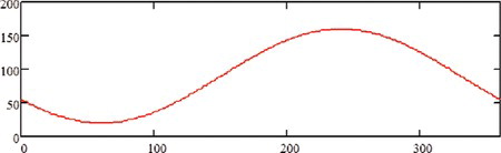
The light intensity of a point in an interferogram modulates accordingly to a cosine function, as in Equation (1). This model is suitable for both interferograms obtained from smooth surfaces as well as for speckle interferometry and also for simple sinusoidal fringe projection.^{[ 11 , 12 ]} The quantity A is the background intensity and B is the modulation coefficient. The term φ corresponds to the natural phase difference between the interfering beams, and is the unknown quantity to be determined. The term θ corresponds to an artificially applied phase shift between the interfering beams. The function I _(θ) represents the resulting intensity as a function of θ. For every phase variation of 2π a complete cycle is achieved corresponding to one period of the cosine function, as shown in Figure 1.

Figure 1 One period of the cosine function I _θ .

Different pixels from the same interferogram usually present distinct intensity values and, consequently, different A, B and φ values. Therefore, in order to distinguish them, a different subscript index i will be assigned for each pixel, as shown in Equation (2):

2.2. Temporal Phase Shifting

The unknown phase values φ _i can be determined from a sequence of three or more images with known phase shift values. For instance, a sequence of four π/2 phase shifted images is largely employed for phase computation^{[ 13 ]} from Equation (3).

When measurements are carried out in a non-steady ambient, it is not rare to find a real value of the phase shift increment different from the theoretical ideal value. Therefore the phase calculation can present unacceptable errors. However, if the phase shift increments are well known, even if they are non-regular, it is still possible to retrieve reliable phase values using an appropriate algorithm.

3. LISSAJOUS FIGURES

Lissajous figures are a family of parametric 2-D curves frequently used to establish the frequency ratio or relative phase between two sinusoidal signals. They were initially investigated by Nathaniel Bowditch in 1815, and later in more detail by Jules Antoine Lissajous in 1857.^{[ 14 ]} Figure 2 presents four examples of Lissajous figures for harmonic signals with different frequency ratios. To obtain Lissajous figures, both harmonic signals are simultaneously plotted in the same graph. One signal is plotted along the X ₁ (horizontal) axis and the other, along the X ₂ (vertical) axis. If the frequency ratio between both harmonic signals is a rational fraction (formed by integer numbers), closed and stable figures are obtained.

Figure 2 Examples of Lissajous figures for frequency ratios fY/fX of 1/2, 3/2, 3/4 and 1/1, respectively.

If the frequencies of both signals are the same, the resulting Lissajous figure is an ellipsis. If the amplitudes are the same and the phase difference between them is π/2 or −π/2 the ellipsis becomes a circle. The effect of phase difference on both signals is shown in Figure 3. If the phase difference is 0 the ellipsis degenerates to a +45° straight line. If the phase difference is π the ellipsis becomes a −45° straight line.

Figure 3 Effect of different phase values (125°, 90°, 45°, 0°) in a 1/1 ration Lissajous figure.

If the light intensities of two different points of an interferogram are plotted in the X ₁ and X ₂ axis while the phase of the interferogram is continuously shifted from 0 to 2π, a Lissajous ellipsis is progressively drawn. The shifted phase value (θ) is the parametric variable. Initially consider a particular case where the two points have π/2 phase difference and the same amplitude in such a way that the Lissajous figure is a perfect circle. When a phase shift Δθ is applied to the interferogram, it produces a rotation of the same amount in a vector with origin at the circle center and end on the circle line. In general, Lissajous figures resulting from two different and randomly selected pixels from a sequence of interferogram a general ellipsis is obtained, as the examples given in Figure 4. Values in each axis vary within the limits 0 and 255 gray levels. The line represents the resulting trajectory produced by continuous variation of the phase shift θ between 0 and 2π. The discrete points on the lines represent the position related to eight discrete θ values. If Δθ is unknown it can be determined from the observed vector rotation on the Lissajous figure. If the Lissajous figures are prefect circles, the relationship between Δθ and the vector rotation is straight-forward. Otherwise, the ellipsis equation must be determined and the rotation computed from that. That is the main idea behind this article.

Figure 4 Lissajous figures resulting from different pixels of the same interferogram.

3.1. Generalized N-Dimensional Lissajous Figures

To improve the robustness of the approach, the authors introduce the concept of generalized N-dimensional Lissajous figures. Instead of using only the X ₁ X ₂ plane, additional dimensions can be added. For example, if the light intensity of a third point in the interferogram is now associated with the X ₃ axis, that is perpendicular to X ₁ and X ₂ , a 3-D Lissajous figure is constructed.

In three dimensions, Lissajous figures would be formed by three cosine signals with different parameters, one for each orthogonal axis (X₁, X₂ and X₃). So, the 3-D Lissajous figures equations as a function of the j-th phase increment θ _j are:

Since they have the same frequency, the resulting figure in the 3-D space will be a line shaped as an ellipsis. It was verified that the resulting 3-D ellipsis is not a true 3-D line, but it is entirely contained in a 2-D plane inclined with respect to the orthogonal axis. The point position in the 3-D space will follow the 2-D ellipsis path as θ varies from 0 to 2θ. It is convenient to use a base formed by two orthogonal vectors, from the ellipsis plane, to describe the discrete point locations on the ellipsis plane. Let P ₁ to P _K be K tridimensional vectors. They represent K points along the ellipsis line which coordinates are given by Equation (5), as functions of the “j-th” phase increment θ _j . The index j stands for the image sequence numbering and ranges from 1 to K.

To determine a orthogonal vectors base lying on the ellipsis plane three non collinear points P _a , P _b and P _c are selected. The difference vectors Δ _ab and Δ _ac are formed as:

The first unitary coplanar vector is normalized by:

The second coplanar unitary vector, and also orthogonal to the first one, is obtained by:

The respective coordinates projected on the plane will be established by:

Therefore, the projected values (XP _j , YP_j) result in a set of 2-D coordinates for each 3-D point.

When N > 3 points are taken from each image of the sequence, the signal of each selected point is assigned to a new orthogonal axis and an N-dimensional Lissajous figure is obtained. Also in this case, it was verified that the resulting N-dimensional line is entirely contained in a 2-D inclined plane. The choice of N will be discussed latter. The values assigned to each of the N axis are:

Therefore, one N-dimensional vector will be formed for each one of the K images of the sequence. N is the number of selected points in each image. The corresponding phase increment θ _j for each image are the unknowns to be determined.

At the end, K N-dimensional points will be available for a set of K interferograms. They are projected in the ellipsis plane in a way similar to the one discussed in equations 6 through 9, and a set of bi-dimensional points will be available: XP_j and YP_j, where j ranges from 1 to K.

The choice of greater values of N produces a more robust estimation of the unknown θ _j values. It reduces the probability to the ellipsis degenerate into a 45° inclined line. It also reduces the influence of random errors due to electronic noise or bad modulating pixels since a much larger amount of data is used. The computational cost of increasing N is negligible. Values ranging from 150 to 2500 have shown very good results. Best results are obtained choosing pixels with higher modulation (B _i ) values. The selection of good modulating points can be done just selecting points with larger intensity spans among the image sequence.

3.2. Ellipsis Fitting and Phase Determination

To compute the relative phase increments θ _j , the corresponding ellipsis equation must be determined from the set of K projected points coordinates XP _j , YP _j . From that it is possible to compute the angles of the vectors starting in the ellipsis center and pointing to each of the K projected points. Each individual angle value depends on the choice of the orthogonal basis. However, the angular differences between them (phase increments) are invariants.

The resulting figure of the N-dimensional Lissajous figure projected on the plan can be described by the general equation of the ellipsis.^{[ 15 ]} Its parametric representation in polar coordinates is:

Where:

	XC and YC: coordinates of the ellipsis center
	R1 and R2: maximum and minimum values of the radii of the ellipsis
	θ: polar angle expressed in the trigonometric direction and origin on the horizontal axis
	ϕ: angle formed between the X axis and the angle of the maximum radius of the ellipsis.

Equation (12) can be expressed in the Cartesian form:

Once the six above coefficients are found, it is possible to compute the geometrical parameters of the ellipsis through the following relations:

	(a) Coordinates of the ellipsis center:
	(a) Main radii:
	(b) Angle of the main radius of the ellipsis:
	(c) θ angle of a given point (x0, y0) on the ellipsis line is computed by:

Fitting a general ellipsis equation to a set of discrete data it is not a trivial task. A very effective and robust approach is presented by Fitzgibbon at al.^{[ 16 ]} The starting point is a set of K points ideally belonging to the ellipsis. A minimum of six non collinear points should be required since six parameters must be determined. However, mathematical constraints reduce the problem to five degrees of freedom. Therefore, a minimum of five non collinear points is sufficient.^{[ 16 ]} Let XP _j and YP _j be the coordinates of the K points. To use a more compact notation, let x _j  = XP _j and y _j  = YP _j . The first step is arranging a data matrix within a six columns and K rows matrix:

Then, a symmetric matrix is formed by multiplying G by its transpose:

Finally, since not all parameters are independent, a constraint matrix D should be used to guarantee that the resulting equation is one ellipsis. This constraint 6 × 6 matrix is given by the following elements:

After that, the generalized eigenvalues and eigenvectors resulting from the system formed by matrices S and D are computed. The smaller non infinite eigenvalue is searched. The elements of the eigenvector corresponding to the smaller eigenvalue (negative and numerically non infinite) are the coefficients values a, b, c, d, f and g which define the Cartesian parameters of the equation of the ellipsis.

3.3. Phase Calculation from Irregularly Phase Shifted Images

Since the ellipsis equation is determined the unknown phase shifts θ _j are determined for each image of the sequence by Equation (17), the phase value can be determined for all remaining points of the images. A phase calculation equation for K irregular phase shifts is also presented in this article.

Let I _j (x, y) be the intensity distribution of the j-th interferogram, where j = 1 to K. Let's assume that all the phase shift value θ _j were previously determined for each j-th image from the N-dimensional Lissajous figures. The phase values φ(x, y) for each pixel (x, y) of the image can be determined from Equation (21). The coordinates (x, y) were suppressed for compactness.

The quantities on equation are computed from image intensities I _j (x, y) and phase shift value θ _j as follows. All the summations are ranging from j = 1 to K:

4. ALGORITHM VALIDATION

A minimum of five phase shifted images, with different phase shifts, is required. However, larger number of images results in redundancy, which is beneficial from a statistical point of view. In the first example, a sequence of six synthetic images with a set of sinusoidal parallel fringes was used to validate the proposed algorithm. A 60° phase shift was applied between each one. A region of interest was defined over an area with 20 × 15 points located around the center of the images and all pixels where used to build a 300-dimensional ellipsis. Figure 5 shows the six synthetic images as well as the obtained projected ellipsis. Each point on the ellipsis corresponds to a different image of the sequence. The relative phase shifting among the fringe pattern images were computed using Equation (17). It can be clearly noted in Figure 5 that the computed phase shifts values are accurately equal to 60° as ideally it supposed to be. The phase map was computed using the determined phase shifts values and Equation (21).

Figure 5 Synthetic images used to validate the proposed algorithm.

5. EXPERIMENTAL VERIFICATION

5.1. Fringe Projection Application

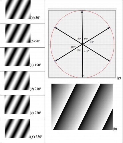
A first practical experiment was accomplished to validate the approach proposed in this article. A LCD projector was used to project a sequence of seven images with parallel sinusoidal fringes on a test piece. The reference phase shift values where 0°, 45°, 90°, 135°, 180°, 270°, and 315°. The images were acquired by a CCD camera with 1280 × 960 pixels and are shown in Figure 6.

Figure 6 (a) to (g) Fringe patterns images with respective phase increments; (h) Phase map computed by the proposed method.

A region of interest with 50 × 50 points has been selected for phase increments calculation. The Lissajous figure resulting from the processed phase increments is shown in Figure 7. Note that increments are non-uniform and there is a jump of 90° between the (e) and (f) images. Figure 6(h) shows the resulting phase map for all the image computed using the phase increments obtained by the proposed method (shown in Figure 7) and Equation (21). Even on presence of irregular phase steps and non-linearity errors of the fringe projection and camera system, the proposed algorithm is able to compute the phase map correctly.

Figure 7 Phase increments computed by the Lissajous method and the respective Lissajous figure.

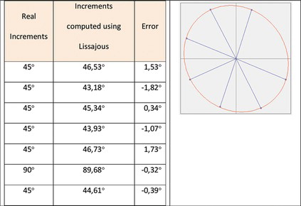
Figure 8 shows a comparison between Lissajous method and a conventional 4-Phase Shifting Method (Equation (3)). In order to make a fairer comparison, just five shifted images were used to compute the phase map by Lissajous method, and four 90° phase shifted images in were used to compute the phase map by 4-Phase Shifting Method. Both maps are shown in Figure 8(a) and (b), respectively. Figure 8(c) and Figure 8(d) show the amplified regions of the phase maps, and Figure 8(e) and figure 8(f) show the respective phase profiles. Comparing the images and its respective phase profile graphs obtained from both methods, the non-linearity found in the phase profile of the Figure 8(f), resulting from 4-Phase Shifting Method, demonstrates that this method is more susceptible to phase step errors than the proposed method.

Figure 8 (a) Phase map computed by the proposed algorithm using 5 shifted images; (b) Phase map computed using 4-phase shifting algorithm; (c) and (d) Amplified regions of the phase maps; (e) Phase profile graph obtained from Lissajous phase map; (f) Phase profile graph obtained from 4-phase shifting map.

5.2. Shearography Application Using Mechanical Load Excitation

An application example is given using a sequence of phase shifted images obtained from shearography with mechanical loading. The surface of an aluminum pressure vessel was used to validate the proposed method. The surface was loaded and analyzed in two states; before and after pressurization. A sequence of seven 45° phase shifted images was acquired before the mechanical loading and another similar sequence was acquired after the mechanical loading. The phase shifts where applied by a piezoelectric transducer (PZT).

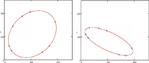
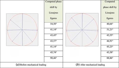
A region of interest was defined over an area and a total number of 30 × 30 points were selected inside the region of interest to compute the phase increments. The 900-dimensional ellipsis was computed and analyzed. Figure 9 shows the resulting projected ellipses computed for each sequence of images, before and after mechanical loading. Each point on the ellipses corresponds to a different interferogram. The relative phase shifting among the interferograms can be computed after least square fitting of the ellipses and using Equation (17). Figure 9 also shows the phase shift values computed for each sequence of images. The computed values have some differences from the ideally expected phase shift values applied by the PZT. These differences are probably caused by the non-linearity of the PZT. However, the resulting phase difference map is not by those supposed PZT errors.

Figure 9 (a) Lissajous figure obtained from sequence of images acquired before mechanical loading and the respective phase increments values, (b) Lissajous figure obtained from sequence of images acquired after mechanical loading and the respective phase increments values.

The phase value was computed for each image pixel using the computed phase shifts and Equation (21). Finally the wrapped phase differences were computed for each image pixel as shown in Figure 10.

Figure 10 (a) Phase map before mechanical loading, (b) Phase map after mechanical loading, (c) Difference phase map.

5.3. Shearography Application Using a Thermal Loading

The last application shows the proposed approach applied to a shearography inspection using a thermal loading. A protective layer of composite material applied over a steel surface was tested for adhesion defects. The surface was heated-up by about 10°C and it was analyzed while it was cooling down. A sequence of phase shifted images was obtained. An ideal phase shift of 90° was applied by a piezoelectric transducer (PZT) before a new image was acquired. However, due to thermal currents, PZT non-linearity and other instabilities, the resulting phase shifts were no longer accurately known. Therefore, no previous assumption on the phase shifts values was used at all.

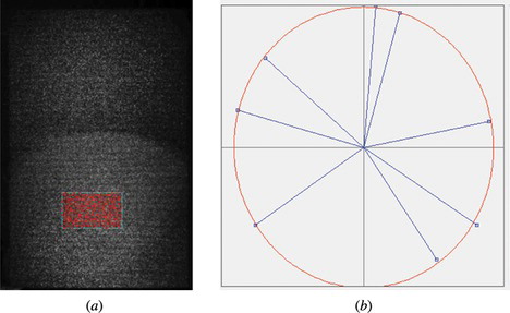
A region of interest, shown in Figure 11(a), was defined over an area where high gradient deformations were not expected. A set of K = 8 initial images was analyzed by a software that implements the developed approach. A total number of N = 300 points were selected inside the region of interest based on their maximum intensity variation ranges. The 300-dimensional ellipsis was computed and analyzed. Figure 11(b) shows the resulting projected ellipsis. Each point on the ellipsis corresponds to a different interferogram. The relative phase shifting among the interferograms can be computed after least square fitting of the ellipsis and using Equation (17). It can be clearly noted in Figure 11 that the real phase shifts were not accurately equal to 90° as ideally it supposed to be. The phase value was computed for each image pixel using the computed phase shifts and Equation (21). The data processing time is almost instantaneous.

Figure 11 (a) Shearography image and the defined region of interest with 300 points used to compute the phase increments; (b) 2-D projection of the N-dimensional ellipsis from a set of eight shearography images with unknown phase shifts.

Another set of K = 8 images was acquired after the test surface had cooled down. The same procedure was repeated, another ellipsis was fitted and the phase shifts determined. Also here, the phase value for each image pixel were computed from Equation (21). Finally the wrapped phase differences were computed for each image pixel, as shown in Figure 12. Note the high image quality obtained from two sets of non-stable images with unknown phase shifts.

Figure 12 Wrapped phase difference from two sequences of shearography images with unknown phase shifts.

6. CONCLUSIONS

This article presents an alternative approach to compute phase values from a set of five or more unknown phase shifted images. The approach combines data from several good modulation points on the image to form an N-dimensional Lissajous ellipsis. An overall phase shift value is determined from the fitted ellipsis for each interferogram. Finally, the phase shifted values are used to determine the phase value for each image pixel.

The mathematical formulation to phase steps calculus using Generalized N-Dimensional Lissajous was presented in details. Also, a generalized equation for phase calculation from non-uniform phase shifts is presented.

A simulation using synthetic images was made to validate the method and equations. A sequence of synthetic images of parallel fringes shifted by a known phase increment was generated and the real phase shifts were accurately calculated.

A fringe projection experiment was built to show that the proposed method can be used to calculate irregular phase shifts too. A set of projected images with different phase shifted values was generated and projected on a pipeline surface. A camera was used to acquire the sequence of projected images. The results showed that the phase values were precisely calculated and the proposed algorithm is a robust tool to be used in applications that not require a previous knowing of the phase increment. Besides that, a comparison with 4-Phase Shift algorithm was performed and the results demonstrated that the method is less susceptible to the non-linearity present in the fringe projection apparatus.

The last two experiments show shearography applications. The first one was carried out using a static mechanical loading and uses a set of 45° phase shifted images; the second one used dynamic loading and a set of unknown phase shifted images.

All results presented in this work show that the method itself is potentially robust since it uses a large amount of data from each interferogram, reducing the influence of noise and the chances of ill-conditioning. The computational effort to compute the arbitrary phase shifts is virtually negligible. No a priori knowledge of pixel modulation or phase increments is required. The phase increment differences, ranging up to 2°, are acceptable for interferometry in unstable environments. Of course, there are more accurate approaches for in-lab environments.

Many others applications can be still explored. Moiré, DSPI, interferometry are just some other examples. The authors are currently analyzing the behavior of the algorithm more deeply and exploring its applications to pulsed shearography in highly vibrating environments.

Notes

Color versions of one or more of the figures in the article can be found online at www.tandfonline.com/uopt.

REFERENCES

- Millerd , J.E. ; Brock , N.J. ; Hayes , J.B. ; North-Morris , M.B. ; Novak , M. ; Wyant , J.C. Pixelated phase-mask dynamic interferometer . In Proceedings of Fringe 2005 - The 5th International Workshop on Automatic Processing of Fringe Patterns , Stuttgart , Germany; Springer: Berlin, Germany 2005 ; pp. 641 – 647 .
- Koliopoulos , C.L. Simultaneous phase shift interferometer . Advanced Optical Manufacturing and Testing II. SPIE 1991 , 1531 , 119 – 127 .
- Creath , K. Phase shifting speckle interferometry . Appl. Opt. 1985 , 24 , 3053 – 3058 .
- Creath , K. Temporal phase measurements methods . In Interferogram Analysis ; Robinson , D.W. ; Reid , G.T. , Eds.; Bristol : Institute of Physics , 1993 .
- Wang , Z. ; Han , B. Advanced iterative algorithm for phase extraction of randomly phase-shifted interferograms. Opt. Lett. 2004, 29, 1671–1673.
- Hildebrand , A. ; Falldorf , C. ; von Kopylowa , C. ; Bergmann , R.B. A fast; and robust approach to phase shift registration from randomly phase shifted interferograms . Speckle 2012: V International Conference on Speckle Metrology , Vigo, Spain, September 10–12, 2012; Bellingham, Washington, DC; SPIE, 2012 .
- Okada , K. ; Sato , A. ; Tsujiuchi , J. Simultaneous calculation of phase distribution and scanning phase shift in phase shifting interferometry . Opt. Commun. 1991 , 84 , 118 – 124 .
- Cundy , H. ; Rollett , A. Lissajous's figures . In Mathematical Models; , 3rd Ed. ; Tarquin Pub. : Stradbroke , England , 1989 ; pp. 242 – 244 .
- Kinstaetter , K. ; Lohmann , A.W. ; Schwider , J. ; Streibl , N. Accuracy of phase shifting interferometry . Appl. Opt. 1988 , 27 , 5082 – 9 .
- Farrell , T. ; Player , M.A. Phase step measurement and variable step algorithms in phase-shifting interferometry . Meas. Sci. Technol. 1992 , 3 , 953 . doi: 10.1088/0957-0233/3/10/003.
- Steinchen , W. ; Yang , L. Digital Shearography: Theory and Application of Digital Speckle Pettern Shearing Interferometry . SPIE Press : Washington , DC , 2003 .
- Yoshizawa , T. Handbook of Optical Metrology: Principles and Applications . CRC Press : New York , 2009 .
- Gasvik , K.J. Optical Metrology. , 3rd Edition . John Wiley and Sons : England , 2002 .
- Lissajous , J.A. Complete Dictionary of Scientific Biography . 2008 . Available at http://www.encyclopedia.com (accessed July 6, 2014) .
- Weisstein , E.W. Ellipse. Available at http://mathworld.wolfram.com/Ellipse.html (accessed March 13 , 2014 ).
- Fitzgibbon , A. ; Pilu , M. ; Fisher , R.B. Direct least square fitting of ellipses . IEEE Trans. Pattern Anal. Mach. Intell. 1995 , 21 ( 5 ), 476 – 480 .