Characterization of Transducer Performance and Narrowband Transient Ultrasonic Fields in Metals by Rayleigh-Sommerfeld Backpropagation of Compression Acoustic Waves Measured with Double-Pulsed Tv Holography

Abstract

This article presents a method aimed at the characterization of the narrowband transient acoustic field radiated by an ultrasonic plane transducer into a homogeneous, isotropic and optically opaque prismatic solid, and the assessment of the performance of the acoustic source. The method relies on a previous technique based on the full-field optical measurement of an acoustic wavepacket at the surface of a solid and its subsequent numerical backpropagation within the material. The experimental results show that quantitative transversal and axial profiles of the complex amplitude of the beam can be obtained at any plane between the measurement and excitation surfaces. The reconstruction of the acoustic field at the transducer face, carried out on a defective transducer model, shows that the method could also be suitable for the nondestructive testing of the performance of ultrasonic sources. In all cases, the measurements were performed with the transducer working under realistic loading conditions.

NOMENCLATURE

2-D	=	two-dimensional
3-D	=	three-dimensional
c L	=	phase velocity of compression acoustic waves in the material
d	=	reconstruction distance
D	=	diameter of the specimen
h	=	thickness of the specimen
j	=	imaginary unit
k a	=	wavenumber of the acoustic wave
f a	=	central frequency of the acoustic excitation
N	=	number of optical phase-change maps in a experiment
n	=	index that identifies the position of a given map within a sequence
Si	=	identification label for each specimen (i = 1, …, 3)
t	=	time
T a	=	temporal period of the acoustic excitation
x	=	shorthand notation for the position (x,y,z 0) on the measurement surface.
ΔΦ	=	sequence of optical phase-change maps measured at the surface of the specimen
ΔΦ n	=	optical phase-change map at position n in the sequence
	=	sequence of complex-valued maps that are the output of the 3-D Fourier transform phase evaluation stage applied to ΔΦ
n	=	complex-valued map at position n in the sequence
	=	complex-valued map reconstructed within the specimen.
Δt	=	temporal sampling period of the measured acoustic displacement
Δz	=	size of the reconstruction step
λ	=	laser wavelength
λa	=	acoustic wavelength
τexc	=	variable time delay between wave generation and optical probing
τ	=	fixed time delay between laser pulses
ωa	=	central angular frequency of the acoustic excitation

1. INTRODUCTION

The usual approach to investigate the field radiated by acoustic sources such as ultrasonic transducers is the acquisition of experimental data by measuring the pressure distribution in a fluid medium, typically water. This is usually accomplished by using point detectors such as hydrophones that scan the acoustic field^{[ 1 , 2 ]} or arrays of hydrophones. From this kind of measurements, important characteristics of the sound field emitted by the transducer (such as the axial and transversal beam profiles, focal length or beam spread) can be derived. This classical method has certain drawbacks, such as a reduced spatial resolution, the need for time-consuming, careful alignment and re-positioning of the probe, or the fact that the presence of the detector perturbs the measured sound field. Less invasive alternatives use a thin reflective membrane (pellicle) perpendicular to the propagation direction of the acoustic beam and a laser interferometer to measure the displacement or velocity of the ultrasound-driven membrane. Thus, it is possible to obtain quantitative maps related to the 2-D spatial distribution of the acoustic field at different distances from the transducer.^{[ 3 , 4 ]} Truly non-invasive, all-optical alternatives were also developed by using a laser beam oriented orthogonally to the main propagation direction of the acoustic beam. A 2-D projection of the acoustic field on a plane perpendicular to the laser beam can thus be obtained, either with scanning laser vibrometers^{[ 5 , 6 ]} or full-field optical techniques such as TV holography^{[ 7 ]} or Schlieren imaging.^{[ 8 ]} When combined with tomographic techniques, this configuration provides data in three dimensions and thus yields quantitative mappings of acoustic beams.^[ 9-11 ^]

When the measurements yield both the amplitude and phase of the acoustic wave, it can be numerically propagated forwards and backwards from the measurement surface.^{[ 12 ]} The backpropagation of a 2-D set of experimental data, measured at some distance in front of the emitter, is an indirect approach to obtain the acoustic pressure or normal velocity distributions at the transducer surface, which give information about the actual vibration pattern of the device and are valuable for the subsequent modeling of its radiated field. This method has been used, for example, to analyze ultrasonic sources,^{[ 2 , 3 ]} including phased arrays,^{[ 1 , 13 ]} and to assess transducer performance and evaluate its degradation over time.^{[ 14 ]} The experimental data, with few exceptions,^{[ 3 ]} are acoustic pressure measurements performed in water with scanning hydrophones. Optical methods have also been investigated to measure directly the motion of the surface of transducers and piezoelectric films, either with the transducer totally uncoupled,^{[ 15 , 16 ]} or immersed in water, though in this case errors introduced by the acousto-optic interaction between the laser beam and surface waves traveling on the face of the transducer must be taken into account.^{[ 17 , 18 ]}

In practically all cases the transducer is tested and characterized in a reference medium, namely water, which may well be different to the propagating medium of the actual application. In fact, it is likely that the transducer will not even be coupled to a fluid, e.g., in nondestructive testing applications. Therefore, it is interesting to have techniques that provide direct knowledge of the radiated field when the transducer is coupled to a solid propagation medium. Methods based on e.g., Schlieren imaging^{[ 19 , 20 ]} or photoelasticity^[ 21-23 ^] have long been available for visualization of ultrasonic waves within solid materials, and some quantitative results have also been published,^{[ 24 , 25 ]} but their application is restricted to optically transparent media only. Thus, the standardized approach for measurements of beam profiles in solids is the acquisition of pulse-echo signals that arise from the interaction of the sound beam with targets placed in the material, such as metal balls or wires embedded in plastics, or flat-bottom or side holes drilled in metallic blocks.^{[ 26 , 27 ]} However, these measurements are more difficult to perform and provide a sparser set of data than immersion techniques.

To overcome these disadvantages and limitations, we herein propose to use an alternative approach that is based on the full-field optical measurement of a narrowband transient acoustic wave field at the surface of a solid specimen and its subsequent numerical backpropagation within the material. This indirect method to measure an acoustic field inside opaque solid media was initially developed by the authors for the nondestructive testing of inhomogeneous metallic samples,^{[ 28 ]} and it was demonstrated by locating the transversal dimensions and axial position of an internal artificial defect embedded in the material. In the present work, we investigate the feasibility of employing this measurement technique to characterize the transient acoustic field radiated by an ultrasonic plane transducer into a homogeneous isotropic metallic medium, and to obtain the spatial distribution of the acoustic field at the transducer face and thus assess its performance. Some preliminary results of the applications herein explained in detail were presented at the Fringe 2013 Conference.^{[ 29 ]} The validation experiments indicate that our approach may constitute a relevant alternative to solve the problem of characterizing ultrasonic transducers when coupled to metals or other non-transparent solids.

The reconstruction of elastic waves in an isotropic elastic solid medium from data of field components taken on a surface was analyzed by Maginness,^{[ 30 ]} but in that work the measurements were carried out with contact transducers over a sparse sampling grid. This approach has several drawbacks (common to other pointwise contact probes, e.g., accelerometers) such as the need of a coupling fluid, a reduced lateral resolution and an unavoidable alteration of the measurand. By using optical detection, a remote, truly non invasive measurement of the acoustic field can be obtained. In our case, we employ pulsed TV holography to measure, at the surface of the specimen, the spatial and temporal evolution of the displacement field induced by the arrival of successive wavefronts of an acoustic wave packet that has traversed the sample. The primary data set is a sequence of 2-D digital maps of the instantaneous out-of-plane acoustic displacement of the surface of the object, each map corresponding to a different instant. The measurement is thus performed simultaneously at all the points of the field of view with high spatial resolution. The complex acoustic displacement field at the measurement surface is retrieved with a 3-D Fourier transform method applied to the sequence of instantaneous acoustic displacement maps. From the measured complex ultrasonic field, the acoustic amplitude and phase are then numerically reconstructed within the medium with a discrete implementation of the Rayleigh-Sommerfeld diffraction formula.

In principle, the detection of the acoustic field and the measurements required for the backpropagation could be obtained with other methods,^{[ 31 , 32 ]} including well-established non-contact optical methods such as laser Doppler velocimetry (LDV). This is a pointwise technique that provides a very high temporal resolution at each measurement point, but it needs some kind of scanning to inspect a surface, which sets practical constraints on the spatial resolution, mostly to keep acquisition time within reasonable limits. Sampling rates of 1000 points per second^{[ 33 ]} and spatial pitches of 1 mm will be considered as order of magnitude estimates in LDV representative applications. Conversely, TV holography parallelizes the detection by performing simultaneous measurements on a digital sensor with very large spatial resolution (1 Mpixel sensors are common, though cameras up to 50 Mpixel are already commercially available). The measurement time required for LDV to measure over 10⁶ points at a rate of 1000 points per second would be 1000 seconds or about 16 minutes. In our case, a typical experiment comprises one set of 64 maps of size 1 Mpixel that are recorded in about 240 seconds (4 minutes), which is a competitive acquisition time compared to LDV. On the other hand, the minimum measurable displacement obtained with our current prototype is of the order of 1 nm, a modest figure compared to LDV. Nevertheless, pulsed TV holography is a full-field approach that benefits from additional relevant advantages for the measurement of ultrasound, such as true transient analysis capability due to the use of pulsed illumination; a high flexibility in the temporization of illumination and acoustic excitation, which makes it possible to record the holograms before waves scattered or reflected at the specimen boundaries reach the area under inspection, or a field of view easily adjustable over a wide range by changing the imaging optics.^{[ 34 ]}

A detailed description of the optical measurement and wavefront reconstruction technique can be found in the aforementioned Trillo et al.,^{[ 28 ]} yet its essential features and the resultant measured quantities are outlined in Section 2 for the sake of self-containedness. Section 3 explains the details of the experimental procedures, and several examples of the obtained results are presented and discussed in Section 4. The conclusions of the work are summarized in Section 5.

2. THEORETICAL BACKGROUND

The measurement technique can be regarded as a combination of optical, acoustical and numerical methods, and can be divided into four stages: (i) transient insonification of the sample; (ii) full-field optical measurement of the displacement at the surface of the sample; (iii) numerical processing to obtain the acoustic amplitude and phase of the wave at that surface and (iv) numerical backpropagation of the acoustic field within the material.

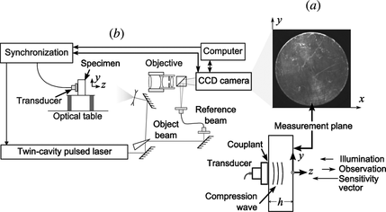
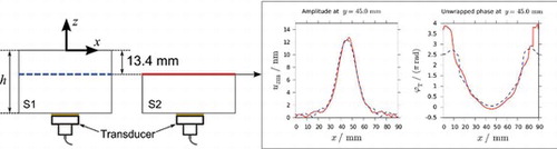
In stage (i), a short burst of compression ultrasonic waves emitted by the transducer is coupled to a thick cylindrical metallic specimen, as shown in Figure 1(a). The quantity subject to measurement, u _z (x, y, z ₀, t), is the out-of-plane displacement of the surface of the specimen at z = z ₀ due to the emerging waves. For simplicity, we have chosen the origin of the z axis at the measurement plane (z ₀ = 0).

Figure 1 Experimental setup and representative solid specimen.

In the general case, displacement in a solid is a vector quantity. Since we are measuring one component only, we are dealing with a scalar problem where attention is confined to the z-component of displacement. With the geometry of our problem, the use of this simplified approach is justified as follows: we assume that the transducer excites fundamentally compression (i.e., P-type) waves in the material, generating a narrow beam (compared to the diameter of the specimen) that propagates in the z direction with small divergence and reaches the measurement surface with a small angle of incidence. On these assumptions, there is no interaction of the incident beam with the lateral walls of the specimen, and the effects of mode conversion (compression waves into shear and surface waves) at the measurement surface are not significant compared to the incident beam. Therefore, we assume that only compression waves are relevant, and that the measurement of the z component of their associated displacement constitutes an adequate representation of the wave field.^{[ 30 ]} The more predominant the z component is, compared to the other (in-plane) components, the more accurate is the information given by this model about the acoustic field and the source that generated it. Finally, the measured displacement u _z at z = 0 is related to the displacement originated by the forward propagating wave alone; due to the boundary conditions, both displacements are proportional (the displacement of the boundary, due to the superposition of the incident and reflected waves, is approximately twice the displacement due to the incident wave alone), and u _z can be described as

where x  = (x, y, 0) is the position on the measurement plane, u _mz ( x , t) is the acoustic amplitude and ϕ_T( x , t) is the total acoustic phase. The latter can be written as ϕ_T( x , t) = ϕ_m( x ) − ω_a t, where ϕ_m is the spatial term of the acoustic phase and ω_a is the central angular frequency.

In stage (ii), two states of the displacement of the object induced by the acoustic wave are recorded with a full-field optical technique, namely double-pulsed TV-holography (also known as electronic speckle pattern interferometry (ESPI), digital holographic interferometry or image-plane digital holography). A sketch of the setup is shown in Figure 1(b). The interference patterns recorded by the camera are processed to yield a digital map of the optical phase-change between these states, ΔΦ _n  = ΔΦ( x , t _n ), which is proportional to the out-of-plane component of the acoustic displacement at instant t _n . When proceeding as explained in Trillo et al.,^{[ 28 ]} this optical phase-change map can be expressed as

The procedure is repeated N times so that a sequence ΔΦ = ΔΦ₁, …, ΔΦ _N of optical phase-change maps is obtained. From one map to the next, the delay τ_exc between the generation of the ultrasound and the emission of the laser pulses is increased by a fixed amount Δt. As τ_exc determines the distance travelled by the wave in the material and, consequently, the part of the wave packet that is captured at the measurement surface, the sequence ΔΦ is a movie-like record of the temporal evolution of the 2-D acoustic displacement at that surface (Figure 2(a)). The measurements that yield the individual maps in the sequence ΔΦ are actually performed on different wave trains; however, the excitation is repeatable, so the final result is equivalent to sampling the same wave train with a temporal sampling period Δt. This value must be chosen short enough, compared to the acoustic temporal period T _a, to ensure the Nyquist sampling condition.

Figure 2 Sketch of the 3-D Fourier transform method. Only three maps are shown for simplicity. An actual sequence would contain a power-of-two number of maps N, typically N = 64 or N = 128. (a) Sequence ΔΦ of optical phase-change maps that contain the spatial and temporal evolution of the out-of-plane displacement at the measurement surface. (b) Complex-valued 3-D spectrum obtained by a 3-D Fourier transform of the sequence in (a); only the modulus is shown. (c) Bandpass filtered 3-D spectrum; only the modulus is shown. (d) Sequence of complex-valued maps that contain the acoustic amplitude and phase at the measurement surface.

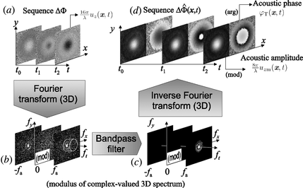
For narrowband excitation, the data in the sequence ΔΦ have spatial variation (in each map ΔΦ _n ) and temporal periodicity (at each pixel along the sequence). Therefore, we apply to these data a specific phase evaluation method based on a 3-D Fourier transform,^{[ 28 , 35 ]} which is graphically summarized in Figure 2. The information of the spatiotemporal acoustic field is separated in frequency space by the intrinsic spatial and temporal carriers present in the data, selected with a 3-D bandpass filter and retrieved in a sequence of complex-valued maps (Figure 2(d)). Each element in the sequence, with n = 1, …, N, is expressed as

and can be regarded as an acoustic hologram with very high spatial resolution. Dense bidimensional maps of the acoustic amplitude and total acoustic phase at the instant t _n are then obtained from each map as shown in the following:

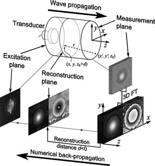
Finally, one of the maps is used as the input for a numerical backpropagation algorithm, which reconstructs the acoustic amplitude and phase within the material by applying a discrete implementation of the general Rayleigh-Sommerfeld diffraction formula^{[ 36 ]}

where λ_a is the wavelength of the acoustic wave, k _a = 2π/λ_a is the wave number, r = [(x–x′)²+(y–y′)² + d ²]^1/2 and stands for the reconstructed acoustic field at a distance d = z − z ₀. This is analogous to the approach used in optical digital holography, but in this case no approximations of the general formula have been used, as the reconstruction distance is comparable to the acoustic wavelength. The input field can be propagated either forwards (d > 0) or backwards (d < 0). In our case, d < 0, as shown in Figure 3. The above integral in Equation (6) can be interpreted as the convolution of the input field with an impulse response function and, therefore, the reconstructed field at a distance d from the measurement surface at z ₀ can then be calculated as a sequence of direct and inverse Fourier transformations. The reconstruction distance can be expressed directly in terms of the z coordinate, since z ₀ = 0, and we will use that notation henceforth; e.g., a map that is backpropagated 3 mm below the measurement plane is said to be located at z = −3 mm.

Figure 3 Geometry of the numerical reconstruction process.

3. EXPERIMENTAL

In this section we describe the main features of the experimental procedure. The essential elements of the set-up, outlined in Figure 1(a), are a twin-cavity, injection-seeded, frequency-doubled, pulsed Nd:YAG laser (model Spectron SL404 T); a modified Mach–Zehnder speckle interferometer with sensitivity to out-of-plane displacements and a CCD camera (PCO SensiCam Double Shutter) capable of recording two frames within a very short time (<1 µs). Each of the laser cavities delivers light pulses with a wavelength of λ = 532 nm at a fixed rate of 25 Hz. The delays between the pulses of both cavities, and between these and the acoustic excitation are accurately controlled with delay generators (Stanford Research Systems DG535) and custom electronics. Light reflected off the specimen interferes with the reference beam on the CCD and is digitized by the camera in two interferograms with a maximum size of 1280 × 1024 pixels and 12 bits per pixel. The reference beam was guided through an optical fiber and displaced slightly off-axis to introduce a spatial carrier in each interferogram, and a controllable aperture in the camera objective was used to adjust the speckle size so that it could be resolved by the sensor.

The results reported here were obtained with three cylindrical, homogeneous aluminium specimens of diameters D and thicknesses h (as shown in Table 1). The specimens were chemically treated with a diluted H₃NO₄ solution to set a matt finish. A single-element, resonant piezoelectric transducer (manufactured by TECAL S. A.), with a plane surface of diameter 20 mm, was coupled concentrically to each specimen with honey. When excited by a high voltage signal, the transducer launched short bursts of compression waves with a programmable number of cycles per burst and a central frequency f _a = 1/T _a = (1.00 ± 0.01) MHz, which is the peak of the frequency spectrum of the transducer's piezoelectric crystal. The phase velocity c _L of the compression acoustic waves in the different samples was measured by pulse-echo, and the acoustic wavelength in the material was calculated as λ_a = c _L/f _a. The values obtained for each specimen are summarized in Table 1.

Table 1. Experimental values of the dimensions, acoustic wavelength and phase velocity for f _a = (1.00 ± 0.01) MHz in each specimen. The number of cycles per excitation burst used in the experiments is also displayed. All expanded uncertainties are determined with a coverage factor k = 2

Specimen	D (mm)	h (mm)	c L (m/s)	λa (mm)	Number of cycles in the wave burst
S1	140.02 ± 0.04	50.43 ± 0.04	6400 ± 3	6.40 ± 0.07	5
S2	140.08 ± 0.04	37.05 ± 0.04	6397 ± 4	6.40 ± 0.07	5
S3	70.10 ± 0.05	23.37 ± 0.01	6448 ± 6	6.45 ± 0.07	10

We recorded sequences of N = 64 optical phase-change maps ΔΦ _n (n = 1, …, N), where a region of interest of size 1024 × 1024 pixels was selected out of the available sensor size. In all cases, the temporal sampling period was set to Δt = T _a/4 = 250 ns, i.e., the acoustic displacement was sampled four times within each temporal period of the acoustic wave. The separation between laser pulses was set to τ = 1.5 µs = 3T _a /2.

As we noticed a fluctuation in the background level of the phase maps, a pre-processing stage was applied to the data before proceeding with the 3-D Fourier transform method outlined in Section 2 (see Figure 2). We attributed that fluctuation to slight changes in the relative phases of each pair of laser pulses, which added a random DC level to each phase-change map ΔΦ _n . In frequency space, these phase jumps translated into a spurious signal with zero spatial frequency and a broad temporal spectrum, often broad enough to reach the temporal frequency planes where the true signal was located. Since the spectral content of the wave has low spatial frequency and is symmetrical around (f _x , f _y ) = (0,0), it was not possible to filter out the noise in the 3-D Fourier space without removing part of the signal. To overcome this problem, we calculated the average phase in a square region of side 100 pixels at the lower left corner of each map ΔΦ _n , and subtracted this background phase from all the pixels in the image. This procedure was applied to all the images in each sequence, and then the 3-D Fourier transform of this corrected set was calculated. In frequency space, a circular Hann window of diameter 81 pixels, centered at spatial frequencies (f _x , f _y ) = (0,0), was applied to the f _t planes 12 to 20 of the discrete 3-D spectrum to select one of the side lobes. In the temporal frequency axis, this amounts to a rectangular bandpass filter with 0.75 MHz and 1.25 MHz cutoff frequencies.

To reconstruct the measured field inside the specimen, we choose a map located early in the sequence —typically at position n = 8 to n = 18, depending on the length of the burst—to ensure that we are dealing with first-arriving sound and surface waves have not fully developed. In the different experiments reported here, we used the complex-valued maps at position n = 13 (). For the numerical reconstruction of the measured fields, we used a discrete implementation of the general Rayleigh-Sommerfeld diffraction formula in Equation (6) using a fast Fourier transform (FFT) convolution^{[ 28 ]} with pixel size values of Δx = Δy = 0.0879 mm for samples S1 and S2, and Δx = Δy = 0.0729 mm for the experiments carried out with specimen S3. All the operations were performed in a desktop computer equipped with an Intel Core i7-3770 CPU running at 3.40 GHz and 16.0 GB of RAM memory. The time necessary for calculating and writing to disk the TIFF file that contains the acoustic field reconstructed at a given distance is typically about 0.35 s.

4. RESULTS AND DISCUSSION

In the first experiment, the acoustic field emitted by the transducer was measured at the surface of specimen S1. The complex-valued wavefront located at position n = 13 in the sequence was selected and numerically backpropagated for a set of regularly spaced reconstruction distances, ranging from z = 0 mm to z = −50 mm, with a reconstruction step Δz = −0.1 mm. Figures 4(a) and 4(b) show the maps of acoustic amplitude and phase obtained for a reconstruction distance of 50 mm below the specimen surface.

Figure 4 Maps of (a) the acoustic amplitude and (b) the acoustic phase reconstructed at 50 mm below the surface of specimen S1. (c) Stack of the transversal profiles of acoustic amplitude at y = 45.00 mm—indicated by the arrows in (a)— obtained for all the reconstruction distances. (d) Longitudinal profile of the acoustic amplitude at position (x,y) = (45.00, 45.00) mm. This line is the intersection of the acoustic amplitude surface shown in (c) with a plane perpendicular to the x-axis at x = 45.00 mm. (e) Top-view of the data set of acoustic amplitude shown in subfigure (c). If the acoustic phase is plotted instead of the acoustic amplitude, the result shown in (f) is obtained.

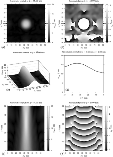
We have thus generated a dense volume of data (≈ 5 × 10⁸ points) that retraces the propagation of that wavefront within the volume of material delimited by the excitation and measurement surfaces. From these data, we can obtain any transversal profile of the beam for each value of z. In this experiment we have chosen the central line at position y = 45.00 mm, indicated by the arrows in Figure 4(a). By plotting the acoustic amplitude along this line for all the values of the reconstruction distance, the evolution of the beam in the material can be determined, as shown in the pseudo-3-D representation of Figure 4(c). Figure 4(e) is a gray-coded, top-view of the same set of data. Also, we can obtain any longitudinal profile by plotting the acoustic amplitude at a fixed position (x, y) for all the values of the reconstruction distance z. Figure 4(d) shows the profile obtained for (x, y) = (45.00, 45.00) mm, near the center of the beam. If we plot the total acoustic phase instead of the acoustic amplitude, we obtain the result shown in Figure 4(f), which uses the same type of representation as Figure 4(e). Column (i) in Figure 5 contains several other maps of the acoustic amplitude obtained in this experiment.

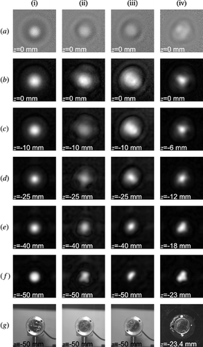
Figure 5 The results obtained in three experiments of simulated defective coupling are shown in columns (ii) to (iv). The maps in columns (ii) and (iii) were obtained with specimen S1. The corresponding results for the same specimen and homogeneous coupling are shown in column (i) for comparison. Results in column (iv) were obtained with the thinnest specimen, S3. Row (a) shows the measured optical phase-change maps, located at position n = 13 in their respective sequences. Row (b) contains the corresponding acoustic amplitude maps (i.e., mod()). Rows (c) to (f) show the acoustic amplitude reconstructed from within the specimen at the distances indicated. Row (g) is a white-light image of the transducer after the specimens were carefully removed. The field of view is 75.6 mm × 75.6 mm in column (iv), and 90.0 mm × 90.0 mm in the other cases.

Figures 4(c) and 4(e) show that the acoustic beam generated by the transducer in good-coupling conditions gets slightly focused—this happens at z ≈ −33 mm, i.e., at 17 mm from the source, where the acoustic amplitude is maximum—and then broadens as the distance from the source increases. This behavior is also observable in Figure 6(i) and in Video1.mp4, which shows the entire sequence of reconstructed acoustic amplitude maps in this experiment and the progressive construction of Figure 4(c), from the measurement surface towards the transducer. This video is the first of the five online supplemental files that accompany this article and can be reached at the publisher's website. The corresponding maps of the acoustic phase can be found in Video2.mp4. These maps and figure 4(f) show that the total acoustic phase of the beam is slightly curved at the measurement surface but is essentially flat at the location of the transducer, that is the expected behavior since the emitter was designed for pure piston motion.

Figure 6 Dashed lines: transversal profiles of acoustic amplitude and unwrapped phase measured at the surface of S1 and then backpropagated within the specimen. Solid lines: transversal profiles of acoustic amplitude and unwrapped phase measured at the surface of the thinner specimen S2. The reconstruction distance was set to −13.4 mm, the difference between the average thicknesses of the samples. Therefore, the reconstructed and measured fields are located at the same distance relative to the transducer.

We carried out three additional experiments to test the capability of this technique to assess the performance of the transducer. The tests were performed on two specimens of different dimensions, namely S1 and S3. To simulate a defective source, we introduced a deliberate acoustic impedance mismatch at the sample-transducer interface by the inhomogeneous application of the couplant. In the first experiment with S1, a very small quantity of honey was applied on the transducer in the shape of a cross. In the second one, with the same specimen, the couplant was applied to half the area of the transducer only. In the third experiment, specimen S3 was used, and the honey was spread in a T-shape, rotated about 45 degrees counterclockwise. The results of each experiment are arranged in columns in Figure 5. Some of the results already presented in Figure 4 and Videos 1 and 2 are shown in column (i); these experiments were conducted with a homogeneous distribution of the couplant fluid, and are provided for comparison purposes. The optical phase-change maps ΔΦ₁₃ of the respective sequences are presented in row (a). Row (b) contains the corresponding acoustic amplitudes at the measurement plane (mod()). The acoustic amplitude reconstructed from at several distances within the samples is shown in rows (c) to (f). In particular, row (f) shows the acoustic field at (or nearly at) the specimen-transducer interface. The white-light images in row (g) indicate the distribution of couplant on the transducer after the specimens were carefully removed. Comparing rows (f) and (g), it is apparent that the reconstructed acoustic amplitude in the immediate vicinity of the transducer closely resembles the shape of the area with an effective acoustic coupling. The complete set of experimental results of the tests reported in columns (ii), (iii) and (iv) of Figure 5 are available online as three MPEG-4 video files (Video3.mp4, Video4.mp4 and Video5.mp4, respectively).

Finally, we proceeded to compare the value of the acoustic field obtained by backpropagation with an equivalent result obtained by measurement, with the aim of verifying whether the reconstructed field was a faithful representation of the actual acoustic field within the material. For that purpose, we used specimens S1 and S2, which have the same diameter and c _L but different thicknesses.

First, the acoustic amplitude and phase were measured at the surface of specimen S2 and, in an independent experiment, they were measured at the surface of S1. The experimental parameters were kept equal in both cases, with the exception of the thickness h of the specimens and τ_exc, the delay between the trigger of the acoustic wave and the emission of the laser pulses. Its value was adjusted to ensure that, in both experiments, the wavepacket was not yet visible in the first few frames of the sequences of optical phase-change maps ΔΦ, i.e., it was just about to emerge at the measurement surface. The acoustic field measured at the surface of S1 was then backpropagated inside the specimen. The reconstruction distance was set to z = −13.4 mm, which is the difference between the average thicknesses of the samples. Both fields (reconstructed in S1 and directly measured in S2) were thus located at the same distance with respect to the emitter and, therefore, expected to coincide in amplitude and, at most, differ in a constant term in the phase. The good agreement between the measured and the numerically backpropagated profiles shown in Figure 6 indicates that, on the assumptions of the wave model stated in Section 2, the reconstructed field does yield a good estimation of the out-of-plane component of the actual acoustic field in the material.

Regarding the amplitude, the average difference between the reconstructed and measured profiles is 0.1 nm. This value is in the order of the standard deviation of the amplitude noise (0.11 nm, which has been computed in a measured amplitude map of specimen S1, in four rectangular regions of 200 × 200 pixels located far enough from the center to ensure that no acoustic wave was present). The standard deviation of the difference between the reconstructed and measured profiles is 0.4 nm, which is approximately 2.5 times the aforementioned standard deviation of the amplitude noise. In the regions where the acoustic amplitude is low, and therefore the signal to noise ratio is small, the disagreement between the measured and reconstructed phase profiles is noticeable, as expected. For values of x between 15 mm and 75 mm, the minimum occurring amplitude in the measured profile is about 0.7 nm, i.e., roughly twice the average of the amplitude noise (0.39 nm, computed in the same regions mentioned above). If we restrict the analysis to this x-interval, the standard deviation of the phase difference is found to be 0.4 rad, which reduces to 0.2 rad for the interval from x = 25 mm to x = 65 mm, where the lower limit of the measured amplitude is about 1.0 nm.

5. CONCLUSIONS

We have reported the experimental validation of a method that provides high-spatial-resolution measurements of the acoustic field radiated by an ultrasonic transducer into a homogeneous isotropic opaque solid medium. The method was tested on three prismatic aluminium specimens of different thicknesses insonicated by a plane resonant piezoelectric transducer of frequency 1.00 MHz. The proposed method is based on the full-field optical measurement of the spatial and temporal evolution of a narrowband transient acoustic wave packet at the surface of a specimen and its subsequent numerical backpropagation within the material.

We have shown that the reconstructed complex acoustic amplitude can be obtained at any plane within the volume delimited by the measurement and excitation surfaces. Therefore, a 2-D set of planes can be generated, which constitutes a 3-D quantitative mapping—both in amplitude and phase—of the propagation of the ultrasonic beam across the solid. From this volume of data, transversal and axial beam profiles at any position within the volume can be obtained, and expected features of the beam such a slight focusing and subsequent divergence are observable from the representation of these data.

We have used the reconstruction of the acoustic field at the excitation surface to assess the performance of the transducer. Artificial models of defective sources with anomalous emission patterns were simulated by the inhomogeneous application of the coupling fluid, leaving large areas of the transducer acoustically uncoupled from the sample. The backpropagation of the measured field to the transducer face yielded acoustic amplitude patterns that were in good agreement with the active (well-coupled) areas of the transducer.

Finally, we have verified the reliability of the backpropagated data by comparing the acoustic field measured directly on the surface of a specimen against the field measured at the surface of a thicker specimen and backpropagated to the same distance relative to the transducer. A good agreement between those fields was found, and on this basis it can be reasonably said that the method renders an accurate description of the actual ultrasonic field within the material whenever the restrictions stated in Section 2 are fulfilled. Therefore, the proposed method might be useful for the characterization of narrowband ultrasonic bursts that propagate with small divergence in solid opaque media and could also be suitable for the nondestructive testing of the performance of ultrasonic sources, with the additional benefit that, in all cases, the measurements are performed with the transducer working under realistic loading conditions.

Notes

Color versions of one or more of the figures in the article can be found online at www.tandfonline.com/uopt.

BRIEF DESCRIPTION OF THE SUPPLEMENTAL CONTENT (VIDEOS)

Video 1: On the left: Sequence of 2-D maps of the acoustic amplitude within specimen S1 obtained by the numerical backpropagation of the acoustic field measured at the surface of the sample (an aluminium cylinder 50.43 mm thick). Size of the reconstruction step: Δz = −0.1 mm. The transversal profiles of the acoustic amplitude at the position indicated by the arrows are shown on the right, and stacked to form a pseudo 3-D representation of the evolution of the beam in the solid material. A top-view of these data is shown at the end of the video.

Video 2: Sequence of 2-D maps of the acoustic amplitude (left) and total acoustic phase (right) reconstructed within specimen S1 by the numerical backpropagation of the acoustic field measured at the surface of the sample (an aluminium cylinder 50.43 mm thick). Size of the reconstruction step: Δz = −0.1 mm.

Video 3: Sequence of 2-D maps of the acoustic amplitude (left) and total acoustic phase (right) reconstructed within specimen S1 by the numerical backpropagation of the acoustic field measured at the surface of the sample (an aluminium cylinder 50.43 mm thick). A deliberate acoustic impedance mismatch (due to the inhomogeneous application of the couplant) was introduced at the specimen-transducer interface to simulate a cross-shaped coupling defect. The distribution of coupling fluid at the face of the transducer after the experiment is shown in a white-light image at the end of the video. Size of the reconstruction step: Δz = −1 mm.

Video 4: Sequence of 2-D maps of the acoustic amplitude (left) and total acoustic phase (right) reconstructed within specimen S1 by the numerical backpropagation of the acoustic field measured at the surface of the sample (an aluminium cylinder 50.43 mm thick). A deliberate acoustic impedance mismatch (due to an inhomogeneous application of the couplant) was introduced at the specimen-transducer interface to simulate a D-shaped coupling defect. The distribution of coupling fluid at the face of the transducer after the experiment is shown in a white-light image at the end of the video. Size of the reconstruction step: Δz = −1 mm.

Video 5: Sequence of 2-D maps of the acoustic amplitude (left) and total acoustic phase (right) reconstructed within specimen S3 by the numerical backpropagation of the acoustic field measured at the surface of the sample (an aluminium cylinder 37.05 mm thick). A deliberate acoustic impedance mismatch (due to an inhomogeneous application of the couplant) was introduced at the specimen-transducer interface to simulate a T-shaped coupling defect. The distribution of coupling fluid at the face of the transducer after the experiment is shown in a white-light image at the end of the video. Size of the reconstruction step: Δz = −1 mm.

REFERENCES

- Schafer , M.E. ; Lewin , P.A. Transducer characterization using the angular spectrum method . J. Acoust. Soc. Am. 1989 , 85 , 2202 – 2214 .
- Alles , E.J. ; van Dongen , K.W.A. Iterative reconstruction of the transducer surface velocity . IEEE Trans. Ultrason. Ferroelectr. Freq. Control 2013 , 60 , 954 – 962 .
- Higgins , F.P. ; Norton , S.J. ; Linzer , M. Optical interferometric visualization and computerized reconstruction of ultrasonic fields . J. Acoust. Soc. Am 1980 , 68 , 1169 – 76 .
- Royer , D. ; Casula , O. Quantitative imaging of transient acoustic fields by optical heterodyne interferometry. Ultrasonics Symposium, 1994. Proceedings 1994 IEEE: 1994, 1153–1162 .
- Wang , Y. ; Theobald , P. ; Tyrer , J. ; Lepper , P. The application of scanning vibrometer in mapping ultrasound fields . J. Phys.: Conf. Ser. 2004 , 1 , 167 – 173 .
- Harland , A.R. ; Petzing , J.N. ; Tyrer , J.R. Nonperturbing measurements of spatially distributed underwater acoustic fields using a scanning laser Doppler vibrometer . J. Acoust. Soc. Am. 2004 , 115 , 187 – 195 .
- Rustad , R. ; Lokberg , O.J. ; Pedersen , H.M. ; Klepsvik , K. ; Storen , T . TV holography measurements of underwater acoustic fields . J. Acoust. Soc. Am. 1997 , 102 , 1904 – 1906 .
- Zanelli , C.I. ; Howard , S.M. Schlieren metrology for high frequency medical ultrasound . Ultrasonics 2006 , 44 , e105 – e107 .
- Bahr , L. ; Lerch , R. Beam profile measurements using light refractive tomography . IEEE Trans. Ultrason. Ferroelectr. Freq. Control 2008 , 55 , 405 – 414 .
- Rustad , R. Acoustic field of a medical ultrasound probe operated in continuous-wave mode investigated by TV holography . App. Opt. 1998 , 37 , 7368 – 7377 .
- Caliano , G. ; Savoia , A.S. ; Iula , A. An automatic compact Schlieren imaging system for ultrasound transducer testing . IEEE Trans. Ultrason. Ferroelectr. Freq. Control 2012 , 59 , 2102 – 2110 .
- Stepanishen , P.R. ; Benjamin , K.C. Forward and backward projection of acoustic fields using FFT methods . J. Acoust. Soc. Am. 1982 , 71 , 803 – 812 .
- Clement , G.T. ; Hynynen , K. Field characterization of therapeutic ultrasound phased arrays through forward and backward planar projection. J. Acoust. Soc. Am. 2000, 108, 441–446.
- Wu , X. ; Worthington , A.E. ; Gertner , M.R. ; Hunt , J.W. ; Sherar , M.D. Characterization of changes in therapeutic ultrasound transducer performance over time using the angular spectrum method . IEEE Trans. Ultrason. Ferroelectr. Freq. Control 2007 , 54 , 1028 – 1035 .
- Duxbury , D.J. ; Russell , J.D. ; Lowe , M.J.S. Accurate two-dimensional modelling of piezo-composite array transducer elements . NDT&E Int. 2013 , 56 , 17 – 27 .
- Tendela , L.P. ; Federico , A. ; Kaufmann , G.H. Evaluation of the piezoelectric behaviour produced by a thick-film transducer using digital speckle pattern interferometry . Opt. Las. Eng. 2011 , 49 , 281 – 284 .
- Sapozhnikov , O.A. ; Morozov , A.V. ; Cathignol , D. Piezoelectric transducer surface vibration characterization using acoustic holography and laser vibrometry. In Ultrasonics Symposium, 2004 IEEE, vol. 1; 23–27 Aug. 2004; pp. 161–164 .
- Certon , D. ; Ferin , G. ; Bou Matar , O. ; Guyonvarch , J. ; Remenieras , J.P. ; Patat , F. Influence of acousto-optic interactions on the determination of the diffracted field by an array obtained from displacement measurements . Ultrasonics 2004 , 42 , 465 – 471 .
- Hall , K.G. Observing ultrasonic wave propagation by stroboscopic visualization methods . Ultrasonics 1982 , 20 , 159 – 167 .
- Baborovsky , V.M. Visualisation of ultrasound in solids . Phys. Technol. 1979 , 10 , 171 – 177 .
- McNamara , F.L. ; Rogers , T.F. Direct viewing of an ultrasonic beam in a transparent solid . J. Acoust. Soc. Am. 1953 , 25 , 338 – 339 .
- Hall , K.G. A qualitative evaluation of variable-angle ultrasonic transducers by the photoelastic visualization method . Ultrasonics 1977 , 15 , 245 – 252 .
- Hsu , N.N. ; Chen , G. ; Sansalone , M. Characterization of a piezoelectric transducer coupled to a solid. In IEEE 1987 Ultrasonics Symposium, Denver, USA, Oct 14–16, 1987, pp. 689–692 .
- Ginzel , E. ; Zhenshun , Z. Quantification of ultrasonic beams using photoelastic visualisation. NDT.net 11 (5). 2006. Available at http://www.ndt.net/article/v11n05/ginzel1/ginzel1.htm (accessed April 5, 2014) .
- Nam , Y.H. ; Lee , S.S. A quantitative evaluation of elastic wave in solid by stroboscopic photoelasticity. J. Sound Vib. 2003 , 259 , 1199 – 1207 .
- Ginzel , E.A. ; Hotchkiss , F.H.C. Ultrasonic beam profile modelling . NDT.net 1997. 2 ( 6 ). Available at http://www.ndt.net/article/ginzel/hotchkis/hotchkis.htm (accessed April 5, 2014) .
- ASTM E1065–08. Standard guide for evaluating characteristics of ultrasonic search units .
- Trillo , C. ; Doval , A.F. ; Hernández-Montes , S. ; Deán-Ben , X.L. ; López-Vázquez , J.C. ; Fernández , J.L. Pulsed TV holography measurement and digital reconstruction of compression acoustic wave fields: application to nondestructive testing of thick metallic samples . Meas. Sci. Technol. 2011 , 22 , 025109 .
- Trillo , C. ; Doval , A.F. ; Fontán , L.M. ; Fernández , J.L. ; Rodríguez-Gómez , P. ; López-Vázquez , J.C. Characterization of the sound field generated by an ultrasonic transducer in a solid medium by Rayleigh-Sommerfeld back-propagation of bulk acoustic waves measured with double-pulsed TV holography . In Fringe 2013, 7th International Workshop on Advanced Optical Imaging and Metrology , Nürtingen, Germany, September 10–13, 2013 ; Springer , 2013 ; pp. 173 – 178 .
- Maginness , M.G. The reconstruction of elastic wave fields from measurements over a transducer array . J. Sound Vib. 1972 , 20 , 219 – 240 .
- Lee , J-R. ; Shin , H-J. ; Chia , C.C. ; Dhital , D. ; Yoon , D-J. ; Huh , Y-H. Long distance laser ultrasonic propagation imaging system for damage visualization . Opt. Las. Eng. 2011 , 49 , 1361 – 1371 .
- Ruzzene , M. Frequency–wavenumber domain filtering for improved damage visualization . Smart Mater. Struct. 2007 , 16 , 2116 – 2129 .
- Castellini , P. ; Martarelli , M. ; Tomasini , E.P. Laser doppler vibrometry: Development of advanced solutions answering to technology's needs. Mech. Syst. Signal Pr. 2006, 20, 1265–1285.
- Fernández , J.L. ; Doval , A.F. ; Trillo , C. ; Deán , J.L. ; López , J.C. Video ultrasonics by pulsed TV holography: a new capability for non-destructive testing of shell structures . Int. J. Optomechatronics 2007 , 1 , 122 – 153 .
- Trillo , C. ; Doval , A.F. Spatiotemporal Fourier transform method for the measurement of narrowband ultrasonic surface acoustic waves with TV holography. In Speckle06: Speckles, from grains to flowers, Proceedings of SPIE 6341, Nîmes, France, Sep 13–15, 2006; pp. 63410 M-1-6 .
- Shack , R.V. ; Harvey , J.E. An investigation of the distribution of radiation scattered by optical surfaces, Final Report, Optical Sciences Center, University of Arizona. 1975. Available at http://www.dtic.mil/dtic/tr/fulltext/u2/a020685.pdf (accessed April 5, 2014) .