Stacking ensemble transfer learning based thermal displacement prediction system

Abstract

In the precision machining industry, machine tools are usually affected by various factors during machining, and various machining errors generated accordingly. Where thermal error is one of the most common and difficult to control factors for machine tools. Therefore, in this study, six temperature sensors and an eddy current displacement meter are provided in a machine tool with 4-axis for dataset collection required for the model training, then data are organized and normalized. Next, data are introduced into a variety of learning models and validated by $k$-Fold cross-validation for predicting those nonlinear factors that affect the errors. At the end, predicted results are summarized and compared to find out the best two model with better predictive performance for pre-trained model of transfer learning. It observes better predicted results from a retraining conducted through applying Multilayer Perceptron (MLP) on these two pre-trained models, wherein MAE value as 0.40, RMSE as 0.52625 and $R^2$ score as 0.99696 respectively.

Keywords:

• Thermal error
• deep learning model
• artificial neural network
• transfer learning

1. Introduction

The precision machining technology of numerical control machine tools is a key development key in the industry. With the advancement of science and technology, precision machining industry has been constantly improving to pursue higher efficiency and higher precision. According to many literatures and machining practices, we know that the accuracy of machining may be affected by many factors. Take one machine tool under conditions of standard, stable and no loaded as an example, due to the defects of manufacturing, assembling, designing, etc on this machine tool, the geometric parameters and positions of the internal components of machine tool may be existed certain difference from their idea values, and such errors are called geometric errors. In addition, during the movement of machine tool, the actual trajectory of the main moving parts such as the spindle and the worktable may be existed certain difference from its ideal one, and such errors are called motion errors. As per the thermal errors, when the numerical control machine tools are affected by many heat sources, such as cutting heat, friction heat, heat generated by the motor due to long-term operation, etc., resulting in the thermal deformation of each component in the machine tool by the internal heat source of machine tool and the temperature change of working environment, thereby generating errors because of changing the relative positions of the internal components in the entire machine tool, and such errors are called thermal errors. Thermal error, a nonlinear feature, is a quasi-static error which is usually deal as static error by technically. A large number of studies have shown that the above errors have caused about 40–70% of total errors on the numerical control machine tools. Obviously, there may be many factors causing errors of machine tools, but in this study, it will focus on the discussion and prediction of thermal errors. Liu et al. proposed one coupling analysis and simulation technology based on finite element thermal structure, wherein temperature field distribution and thermal deformation of spindle were predicted, and predicted results were excellent as compared with the actual results. Now, the most iconic artificial thermal error compensation implemented in the machine tools is found in the product of OKUMA, Japan. Most machine tools are introduced some structural system such as cooling etc. to suppress thermal errors, however, such active suppression methods have disadvantages of high cost, strict environment settings for machines and high energy consumption. As a result, in this study, it will discuss and study the intelligent thermal error compensation.^[1]

Thanks to the progress of artificial algorithms in recent years, they have been widely used in daily life, medical, industry, etc. However, before a model of predicting thermal errors is built for the numerical control machine tools, it is necessary to collect datasets regarding temperature and error from the machine tools in advance. In the study proposed by Lee et al., there were 16 temperature sensors provided at main heating positions of a machine tool operating under the rotational speed of 1000 rpm/min and 1400/min, and the temperature was measured once per second. In order to improve the stability of model, it needed to first find out those points of temperature detection where dramatically affecting the thermal deformation of spindle, next reduced these 16 measurement temperature points to 5 by the DBSCAN algorithm and the Pearson Correlation Coefficient, and finally improved robustness and real-time performance of model by the BP neural network modeling method.^[2] In the study proposed by Xiao et al., it used seven temperature sensors and two eddy current displacement meters under the rotational speed of 2000 rpm/min to measure the temperature of spindle system and the thermal errors of the z axis and the y axis, applied the correlation analysis and regression analysis on those temperature and thermal error data to find out the correlation coefficients among these seven temperature sensor points, and worked out feature values and feature vectors of matrix of correlation coefficients based on Principal Components Analysis. In this study, finally, the feature vectors corresponding to the feature values were multiplied with the temperature dataset to generate input parameters for BP neural network modeling. Sometimes unexpected vibrations might occur during temperature datasets and thermal error datasets collection, resulting in a decrease in predictive accuracy.^[3] Therefore, Makoto et al. proposed Bayesian Dropout to calculate the reliability of uncertainty assessment, wherein it simulated sensor failure by deliberately tampering with temperature measurements for predicting thermal displacement, and predicted the uncertainty accordingly. If the predictive uncertainty was better, the predictive reliability would be worse. In order to suppress the decrease of compensation accuracy, the compensation value was covered with the uncertainty function by adjusting the parameters of moving average filter to smooth the compensation value. This method is not only suitable for ambient temperature changes, but also for thermal errors generated inside the machine tools, as well as for preventing reduction of predictive accuracy caused by sensor failure.^[4] A new temperature measurement system called LATSIS was proposed by Toru et al., which improved the robustness and predictive accuracy of thermal deformation of machine tools by external disturbances like the supply of cutting fluid. This system add a large number of sensors for measuring the temperature of machine tool, so it could measure the three-dimensional temperature distribution of machine tool without the calculation of heat conduction. Toru et al. set 284 sensors in the machine tool, and made prediction of TCP errors based on the temperature measured either with or without the supply of cutting fluid, wherein the predicted results were quite matched.^[5] Jiao et al. proposed the recurrent neural network based on LSTM to predict the short-term energy consumption of non-local residents. In this study, multiple time series related data were used to predict the consumption level of non-local residents, $k$-means was used to analyze the daytime consumption level of non-local residents, and Spearman correlation coefficient was used to find out the time correlation of consumption level of non-local residents under multiple time series. Later, data with higher correlation coefficients were introduced into the LSTM recurrent neural network for training, so as to obtain better predicted results accordingly.^[6] JIAN et al. proposed a method based on transfer and deep learning for dynamic frequency prediction of power system after disturbed, and provided an event-based optimal shedding strategy to maintain the system frequency, thereby improving the timeliness of online frequency control.^[7]

Deep learning is a small set in the field of machine learning, where the difference between these two learning structures is that deep learning will learn how to extract data features by itself but machine learning not. The artificial neural network algorithm are commonly used in feature learning, and there have been several frameworks based on artificial neural network, such as convolutional neural network, deep belief network, etc. In addition, there is certain progress in the modern semiconductor industry, Meada et al. have verified through tests that the time is significantly speed up while GPU is applied on the calculation of neural networks.^[8] Therefore, deep learning has been widely used in academia and industries in recent years, and many problems either difficult or time consuming have been solved one by one. As a result, in this study, it is intended to predict the thermal error of spindle by deep learning, thereby pushing the numerical control machine tools moving forward to the era of intelligence.

In this study, it will introduce three artificial neural network models, namely Long Short-Term Memory model (LSTM), Gate Recurrent Unit (GRU), a combined model of Convolutional Neural Network (CNN) and LSTM, a combined model of CNN and GRU, and five supervised learning models, namely Decision Tree, Random Forest, Support Vector Regression, and Extreme Gradient Boosting (XGBoost), totally seven models for model training, and finally summarize and compare the predicted results.

In the second section of this study, it will introduce the architecture of study system, covering how to collect dataset, what are included in the experimental and how to process those datasets, as in the third section, it will introduce the pre-processing of datasets, structures of those model algorithms and the parameter settings of each model. For the fourth section, it will introduce the validation method, the experimental results and the evaluation of predicted results. At the final fifth section, it will summarize and compare the predicted results of all models, and discuss the conclusion of this study.

2. System architecture

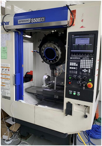
In this study, the training data are taken from thermal compensation experiment of the numerical control machine tool with 4-axis, as shown in Figure 1. In this experiment, several temperature sensors are provided inside the machine tool and an eddy current displacement meter is provided under the spindle to record temperature change of each point as well as the displacement of the spindle caused by temperature change during the long-term operation of the machine tool. Through the above data collection, it can observe the relationship between the thermal error of the spindle and the thermometer provided at each point on the machine tool. Later, in this study, a machine learning model is built to predict the error of the spindle due to the temperature.

Figure 1. 4-axis machine center (S500X1).

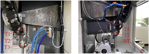
When a numerical control milling machine with 4-axis operates at different rotational speeds, record the temperature at each point and the displacement measured by the eddy current displacement meter every 5 s, then, a dataset is collected. In this experiment, datasets at eight rotational speeds are collected, i.e., total eight datasets are collected. From Figure 2(a)–(h), it shows the trend of temperature and thermal error of each point while the spindle is rotating at 1000 rpm, 2000 rpm, 2500 rpm, 3000 rpm, 5000 rpm, 6000 rpm, 7500 rpm and 9000 rpm, wherein the 6 lines on the upper part of the diagram are the trends of temperature change at 6 temperature points, and the lower part is the displacement change of spindle. Five of the sensors are located around the spindle, and other one sensor is installed on the machine bed, as shown in Figure 3.

Figure 2. Trends of Temperature at Each Point and Thermal Error under Various Rotational Speeds. (a) Trend of Temperature and Thermal Error at 1000 rpm. (b) Trend of Temperature and Thermal Error at 2000 rpm. (c) Trend of Temperature and Thermal Error at 2500 rpm. (d) Trend of Temperature and Thermal Error at 3000 rpm. (e) Trend of Temperature and Thermal Error at 5000 rpm. (f) Trend of Temperature and Thermal Error at 6000 rpm. (g) Trend of Temperature and Thermal Error at 7500 rpm. (h) Trend of Temperature and Thermal Error at 9000 rpm.

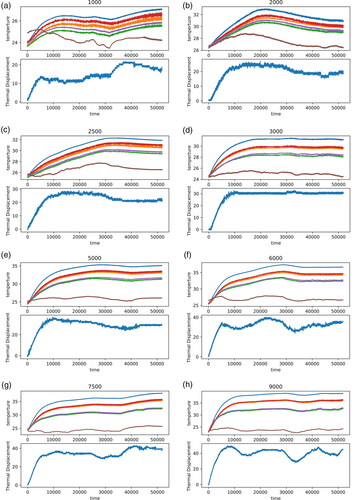
Figure 3. Sensor’s position.

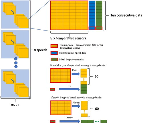
The total time for dataset collection under each rotational speed is 12 h, one data recorded every 5 s, so there are 8640 data of one rotational speed. To emphasize such dataset featured with time series, in a dataset under one rotational speed, take the first data and the following 9 data for summarizing them into a new data, and then take the second data the following 9 data for summarizing them into another new data, and repeat the above step for all data accordingly. At the end, merge all the summarized data to form a dataset of 8630 × 10 × 6, and also apply the same processing for other datasets under other rotational speeds. Finally, flatten all data to obtain a dataset of 69,040 × 60. If the rotational speed and temperature are directly combined for training, there might be no training effects due to the features of the rotational speed data not obvious. Therefore, in this study, during training the neural network model, the corresponding rotational speed for the 10-th data of temperature dataset is taken and converted into a form of one hot code, being the second input training dataset. Not like neural network with function of inputting multiple data, in a supervised learning model, it puts three identical numbers side by side into a one-dimensional array while building a temperature dataset, so that a training set of 69,040 × 3 will be obtained. Combining former training set with the temperature training dataset, a dataset of 69,040 × 63 is formed accordingly. As per collecting thermal error data, the corresponding the 10-th data of temperature dataset is taken to be the label during training, and finally a label dataset of 69,040 × 1 is obtained, as shown in Figure 4.

Figure 4. Schematic diagram of model dataset.

3. The proposed method

Before training the prediction model, the datasets are normalized,^[9] so that the prediction model can be converged much quickly for obtaining better weights during training. Normalization is a method of scaling the value range of the original data to [0,1], which is able to speed up the convergence of models significantly as well as improve the accuracy of models. Its equation is shown as follows: (1) $$X_{\mathit{normalize}}=\frac{x-x_{\min }}{x_{\max }-x_{\min }}\in \left[0,1\right]$$(1) wherein x is the original value, $x_{\min }$ and $x_{\max }$ are the minimum and maximum values of the data, respectively.

Due to imbalanced value distribution in the datasets sometimes, there may be over reliance on specific training data during model training, thereby causing certain deviations. So, first apply $k$-Fold cross validation^[10,11] to disorder those 69,040 training data and divide them into $k$ equal parts. Next, take each sub-dataset as testing set and leave the remaining $k-1$ sub-datasets as training set. 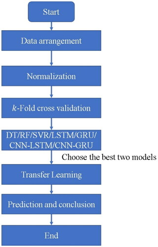After $k$ times training, it will be more objective to evaluate models based on the final summarized results as shown in Figure 5. As all the predicted data organized, start to train these seven different machine learning models, namely, Decision Tree (DT), Random Forest (RF), Support Vector Regression (SVR), Adaptive Boosting (Adaboost), Long Short-term Memory (LSTM), Gate Recuttent Unit (GRU), a combined model of Convolutional Neural Network (CNN) and LSTM, a combined model of CNN and GRU, and Extreme Gradient Boosting (XGBoost), and select two models with better predictive ability as the pre-trained models for transfer learning. At the end, apply the Multilayer Perceptron (MLP) model on top of these pre-trained ones to form transfer learning models. The flowchart of this study is shown in Figure 6.

Figure 5. Schematic diagram of k-Fold cross-validation.

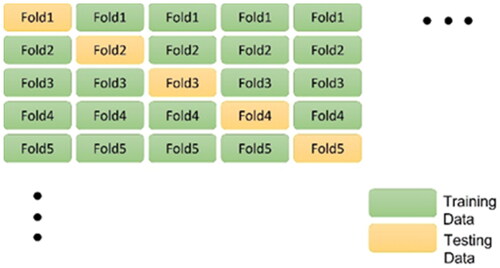
Figure 6. Flowchart of this study.

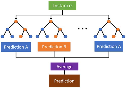
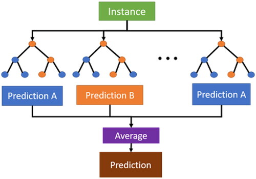
Random Forest (RF)^[13,14] is an improved regression decision tree algorithm as shown in Figure 7. It basically combines multiple CART trees (Classification And Regression Trees, CART)^[15] and carries out a combined learning with Bagging algorithm and Regression decision tree algorithm. During creating a CART, it selects variables for splitting randomly, and keeps former procedure until only one sample parameter left after classification at the final node. As a result, decision trees are differentiated from each other, it means that each tree can make its own prediction through split process of each node from top to down and generate predicted output evenly. Comparing with regression decision trees, RF not only improves its own accuracy, but also addresses overfitting issue. In this study, the number of forest trees is set to 1000, and the maximum depth of trees is set to 12.

Figure 7. Architecture diagram of random forest algorithm.

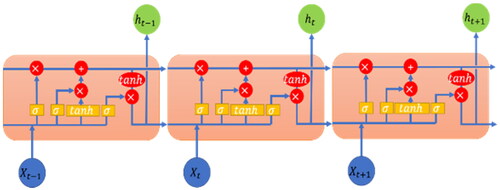
Long Short-term Memory (LSTM)^[19,20] as shown in Figure 8 is an algorithm of Recurrent Neural Network (RNN), which is often used for applications like time series. It mainly works with three gates namely forget gate, input gate and output gate in this algorithm to control whether to update or delete new data. The forget gate will set weights od the concatenate input and the previous output to a value within a range of 0 and 1 through sigmoid function; wherein more data will be forgotten if this value of weight more close to 0, on the contrary, less data will be forgotten if this value of weight more closer to 1. In addition, the input gate will also update weights through sigmoid function but not for weights of the concatenate input and the previous output directly; wherein it first calculates a vector through tanh activation function to determine how many weights need to be updated. At the end, the output gate will obtain the predicted results based on the current input and state through sigmoid function accordingly. A powerful advantage of such recurrent network is that it allows the input and output data to be a sequence of multiple vector sets, so that it can deal with problems by way of single-input single-output, single-input multiple-output, multiple-input single-output, etc. In this study, the rational speed and temperature are used as input respectively, as a result, it can predict the thermal error more effectively by way of multi-input single-output. In this study, five LSTM Layers are provided, and in each LSTM Layer, 16 neurons are provided, tanh is applied as activation function, Sigmoid is applied as activation function for recurring, and a flatten layer is provided for connecting with the second input layer, finally, two Dense Layers are applied for outputting the results; during training, the sample number is set to 30, and the iteration is set as 20 times.

Figure 8. Architecture diagram of LSTM algorithm.

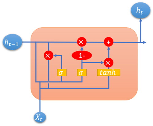
Gate Recurrent Unit is abbreviated to GRU,^[21,22] as shown in Figure 9, which is a similar Recurrent Neural Network (RNN) like LSTM. The difference between these two algorithms is that LSTM is composed of three control gates including forget gate, input gate and output gate for updating or deleting data, but GRU replaces update gate with both input gate and forget gate applied in LSTM, and also combines cell state with hidden state. The training results of GRU and LSTM are similar, the training time of GRU is shorter than thereof LSTM and but the accuracy of GRU is slightly worse than thereof LSTM; therefore, select one of these two models as applicable. In this study, five GRU Layers are provided, 60 neurons are provided in layer 1, 32 neurons are provided in layers 2–4, 16 neurons are provided in layer 5, tanh is applied as activation function, Sigmoid is applied as activation function for recurring, and a flatten layer is provided for connecting with the second input layer, finally, two Dense Layers are applied for outputting the results; during training, the sample number is set to 30, and the iteration is set as 20 times.

Figure 9. Architecture diagram of GRU algorithm.

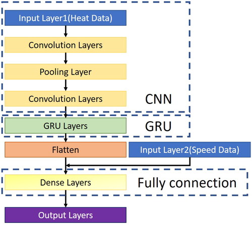
Convolutional Neural Networks Long Short-Term Memory Network, CNN-LSTM,^[23,24] is a combined model which combines Convolutional Neural Network (CNN)^[25] with LSTM. CNN is a typical neural network as shown in Figure 10, which is composed of Convolution Layer, Pooling Layers, Flatten Layer and Fully Connected Layer. Convolution is an algorithm of filtering data by features. It obtain results with different features by setting sizes of the feature detector (filter), and further obtain data with most obvious features by applying Max Pooling method on the pooling layer, thereby obtaining less data without loosing features as well as keeping abilities of noise resistance and calculation reduction.

Figure 10. Architecture diagram of CNN algorithm.

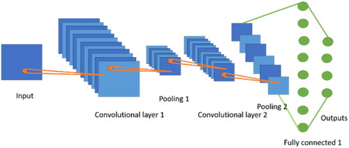
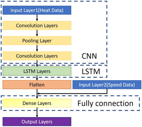
As a result, it can reduce the number of data generated for convolution calculation in the next convolution layer. then convert those two-dimensional data into one-dimensional one by the flatten layer, and at final, apply multi-layer perceptron (MLP)^[26] algorithm on the fully connected layer for calculation. When CNN LSTM is applied in this study, it filters input data by features through CNN, applies LSTM to deal with problems of time sequence, and fully connects layers finally. The architecture diagram of the CNN-LSTM model in this study is shown in Figure 11. In this study, the CNN LSTM model is provided with a one-dimensional convolution layer of 32 neurons, convolution kernel as 3 and activation function as ReLU without filling; a one-dimensional convolution layer 2 of 24 neurons, convolution kernel as 3, and the activation function as ReLU without filling; a layer 3 of pooling layer; a one-dimensional convolution layer 4 of 20 neurons, convolution kernel as 3 and activation function as ReLU without filling; a LSTM recurrent neural network connected with layer 16 neurons in 5 layers; a Flatten to merge with the speed data; and final Dense Layers fully connected with 16, 8, and 1 in three layers for outputting results; during training, the sample number is set to 32, and the iteration is set as 175 times.

Figure 11. Architecture diagram of CNN-LSTM algorithm.

Convolutional Neural Networks Gate Recurrent Unit, CNN-GRU, is a combined model which combines Convolutional Neural Network (CNN) with GRU. This model is similar to the above mentioned CNN-LSTM; first, it filters input data by features through CNN, applies GRU to deal with problems of time sequence, combines speed data input layer and fully connects layers finally. The architecture diagram of the CNN-GRU model in this study is shown in Figure 12. In this study, it is provided with a one-dimensional convolution layer of 48 neurons, convolution kernel as 3 and activation function as ReLU without filling; a layer 2 of 48 neurons, convolution kernel as 3, and the activation function as ReLU without filling; a layer 3 of pooling layer; a one-dimensional convolution layer 4 of 24 neurons, convolution kernel as 3 and activation function as ReLU without filling; a one-dimensional convolution layer 5 of 24 neurons, convolution kernel as 3 and activation function as ReLU without filling; a GRU recurrent neural network connected with layer 16 neurons in 5 layers; and final two Dense Layers for outputting results; during training, the sample number is set to 32, and the iteration is set as 175 times.

Figure 12. Architecture diagram of CNN-GRU algorithm.

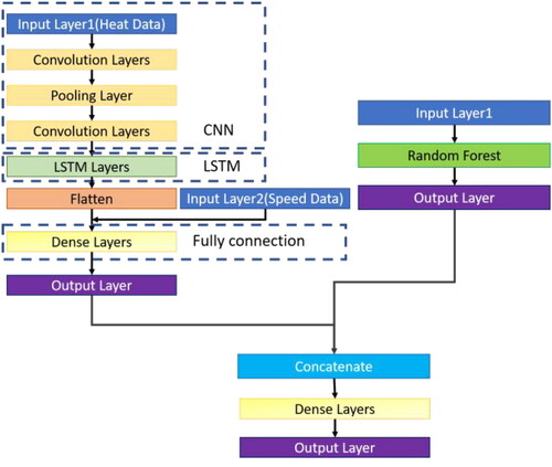
Transfer Learning (TL)^[27,28] is a method of transferring the pre-trained model and parameters to another new model, so that it is not necessary to train a new model from scratch. This method is intended to address those applications with difficult data acquisition and marking. TL can be divided into three categories based on case-sample, features or models. For TL based on case-sample, it assigns weights on the original and the target domain for transfer respectively; if sample data in the original domain is very similar to the those in the target domain, the weights of such samples can be increased. For TL based on features, it will be easier to study the correlation values of the original and the target domain by converting the features of both domains into the same space. And for TL based on models, the most common method in deep learning, it shares parameters between the original and the target domain; in addition, it can obtain better results by fixing the parameters of each layer in the pre-trained model as well as modifying the parameters of some layers. In this study, TL based on case-sample is the basis for modifying the models, while the best two prediction models Random Forest and CNN-LSTM are taken as the pre-trained models for transfer learning. This method optimizes training efficiency and reduces model training time by retaining previously trained model parameters. Additionally, it can achieve the effect of training a model with excellent prediction performance with less data.

In addition, the predicted value of these two models is applied as the training data of the Multilayer Perceptron (MLP) model, which is one kind of neural network, mainly composed of input layer, hidden layer and output layer, as shown in Figure 13. Its calculation process is to transfer the input data to the hidden layer through the input layer, convert them by the activation function, transfer them to the output layer by layer, carry out backpropagation for the output error, calculate the gradient of the loss function for all the weights of the network, and update those weights by the optimizer, thereby reducing the value of the loss function as well as improving the predictive ability. The architecture diagram of Multi Model Transfer Learning Algorithm in this study is shown in Figure 14.

Figure 13. Schematic architecture diagram of MLP algorithm.

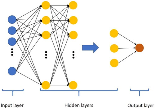
Figure 14. Architecture diagram of multi model transfer learning algorithm.

4. The experimental results

In this study, the thermal compensation datasets of the numerical control machine tool machine tool with 4-axis are divided into 10 equal parts by $k$-Fold, trained by 9 models for 10 times, and carried out with cross-validation in sequence. At the end, the temperature parameters and rotational speed of the thermal temperature of the numerical control machine tool machine tool with 4-axis are input into the model, and the obtained predicted values and actual values are estimated with Mean Absolute Error (MAE), Root-Mean-Square Error (RMSE)^[29] and the Coefficient of Determination ($R^2)$^[30] these three indicators for checking the accuracy of the current prediction model.

Mean Absolute Error (MAE) is one of the linear fractions. It calculates the mean of the residuals directly, so each individual difference has an equal weight on the mean. It is a loss function commonly applied in regression models, which is intended to measure the gap between the predicted value and the actual value. In such evaluation, it can better reflect the actual error of predicted values, wherein smaller MAE, better prediction of the model. The mathematical equation of MAE is shown as follows: (2) $$\mathit{MAE}=\frac{1}{N}{\sum }_{i=0}^N\left|y_i-\widehat{y_i}\right|$$(2) wherein N is the total number of the predicted datasets, $y_i$ is the actual value of the i-th data, and $\widehat{y_i}$ is the predicted value of the i-th data.

Root-mean-square error (RMSE) is also one of the common loss functions applied in regression models, which is often used to evaluate the degree of data change. It takes the difference between the predicted value and the actual value, and calculates the sum of the squares of the former difference, i.e., the root mean square error. Through such square calculation, the penalty for the predicted value that deviates more from the actual value will be larger, so it works better in reflecting the predictive accuracy, wherein smaller RMSE, better accuracy of the prediction model. The mathematical equation of RMSE is shown as follows: (3) $$\mathit{RMSE}=\sqrt{\frac{1}{N}{\sum }_{i=0}^N{\left(y_i-\widehat{y_i}\right)}^2}$$(3) wherein N is the total number of the predicted datasets, $y_i$ is the actual value of the $i$-th data, and $\widehat{y_i}$ is the predicted value of the $i$-th data.

Coefficient of Determination ($R^2)$ is calculated by dividing the sum of squares of residuals by the sum of squares of deviations. This evaluation indicator is often used to check the degree of deviation from the expected values, wherein larger $R^2,$ better predictive accuracy of the model. The mathematical equation of $R^2$ is shown as follows: (4) $$R^2=1-\frac{{\sum }_{i=1}^n{\left(y_i-\widehat{y_i}\right)}^2}{{\sum }_{i=1}^n{\left(y_i-\overline{y}\right)}^2}$$(4) wherein n is the total number of the predicted datasets, $y_i$ is the actual value of the i-th data, and $\widehat{y_i}$ is the predicted value of the i-th data.

In this study, above mentioned three evaluation methods are used to evaluate and summarize the results predicted by 9 models, and the distribution of the actual values and the predicted values are presented in the form of charts for comparison. As shown in Figures 15–23, with distribution of blue, green, and orange points respectively, it is easier to observe those deviations between the predicted values and the actual values, i.e., it is easier to observe the performance of the model by this indicator. (Table 1).

Figure 15. Prediction results of Random Forest. (a) Prediction result (b) Prediction error.

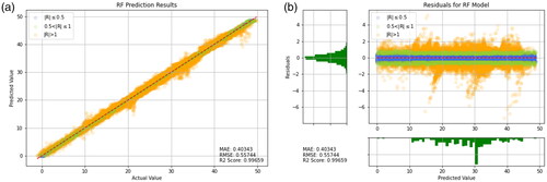
Figure 16. Prediction results of Decision Tree. (a) Prediction result (b) Prediction error.

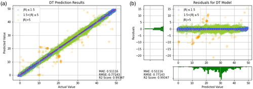
Figure 17. Prediction results of SVR. (a) Prediction result (b) Prediction error.

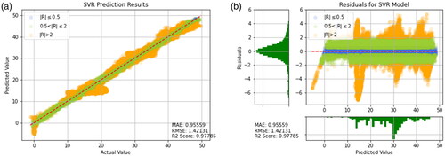
Figure 18. Predicted result of CNN-GRU. (a) Comparison of actual value and predicted value (b) Residual plot.

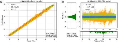
Figure 19. Prediction results of XGBoost. (a) Prediction result (b) Prediction error.

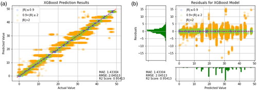
Figure 20. Prediction results of GRU. (a) Prediction result (b) Prediction error.

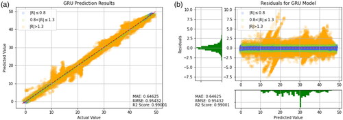
Figure 21. Prediction results of LSTM. (a) Prediction result (b) Prediction error.

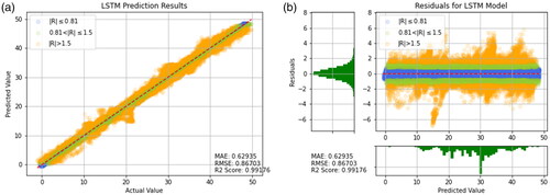
Figure 22. Prediction results of CNN-LSTM. (a) Prediction result (b) Prediction error.

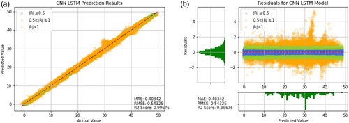
Figure 23. Prediction results of CNN-LSTM + RF (Transfer Learning). (a) Prediction result (b) Prediction error.

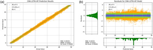
Table 1. Performance of the models.

Model	MAE	RMSE	$R^2$
CNN-LSTM + RF (Transfer Learning)	0.40325	0.52625	0.99696
Random Forests	0.40343	0.55744	0.99659
CNN-LSTM	0.40342	0.54325	0.99676
CNN-GRU	0.43033	0.57263	0.9964
Decision Tree	0.51247	0.7828	0.99328
LSTM	0.62935	0.86703	0.99176
GRU	0.64625	0.95432	0.99001
SVR	0.95559	1.42131	0.97785
XGBoost	1.43304	2.04513	0.95413

As shown in Table 1, it can be observed that Random Forests, CNN-LSTM, CNN-GRU, Decision Tree, LSTM, and GRU have higher R² values, as well as lower MAE and RMSE values. This result indicates good predictive performance of these models. Additionally, Table 2 presents the training results of other models for reference. It can be seen that the predictive ability of the model using the transfer learning method is very well. However, the models in Table 2 are worse than the transfer learning models that include CNN-LSTM and Random Forest. When comparing individual models like Random Forest, Decision Tree, SVR, and XGBoost, it is clear that Random Forest has the best predictive power. Therefore, it is reasonable that applying Random Forest in the context of transfer learning yields the most favorable results. This suggests that when a model has been optimized to its limit, the transfer learning approach proposed in this study can be used to break through bottlenecks by combining two models with better predictive abilities.

Table 2. Additional experiments of the models.

Model	MAE	RMSE	$R^2$
CNN-LSTM + SVR (Transfer Learning)	0.47491	0.63556	0.99557
CNN-LSTM + XGBoost (Transfer Learning)	0.43968	0.5777	0.99634
CNN-GRU + RF (Transfer Learning)	0.45047	0.65101	0.99535
CNN-GRU + DT (Transfer Learning)	0.56836	1.05665	0.98776
CNN-GRU + SVR (Transfer Learning)	0.43581	0.57123	0.99642
CNN-GRU + XGBoost (Transfer Learning)	0.51697	0.69569	0.9949
LSTM + RF	0.85041	1.18879	0.9845
LSTM + DT	0.84218	11.18051	0.98472
LSTM + SVR	0.67146	0.92002	0.99072

After comparing the predictive ability of all models, it can be observed from Figures 16, 19 and 20 that the residual distribution values of the Decision Tree, XGBoost, and GRU models are wider and unequally distributed. Therefore, it can be inferred that these three models have higher prediction errors and hence poorer predictive ability.

According to Figure 15, 17 and 21 it can be observed that the residual distribution ranges of Random Forest, SVR, and LSTM are all between −6 and 6, and the distribution is relatively even. This result indicates superior predictive ability of the aforementioned models. Furthermore, Random Forest exhibits the best predictive performance. In order to highlight the predictive ability of LSTM and GRU, this study additionally employed two combination models, namely CNN-LSTM and CNN-GRU. As shown in Figures 18 and 22 the residual distribution ranges of both models are much smaller than those of the models that use LSTM and GRU alone. The MAE and RMSE values are also much lower than those of the models that use LSTM and GRU alone. This shows that the use of CNN’s feature extraction technique can lead to an improvement in predictive ability.

In order to obtain more accurate prediction results, a combination of the aforementioned superior models and the Random Forest model was employed in this study. Through transfer learning, a better model was obtained with an R² value of 0.9969, RMSE of 0.52625, and MAE of 0.40325.

5. Discussion

After carefully comparing the predicted results of all models, it was observed that the residual distribution of the Random Forest model was between −6 and 4, while the residual distribution of the CNN-LSTM model was between −3 and 5. The transfer learning model combining CNN-LSTM and Random Forest had a residual distribution between −6 and 4, which was consistent with the Random Forest model. However, upon observation, the residual values of the transfer learning model were distributed between −3 and 3, while most of the residual values of the Random Forest model were distributed between −3 and −6. Therefore, the MAE and RMSE values of the transfer learning model were both smaller than those of the Random Forest model. These results also indicate that the transfer learning model is the feasible choice.

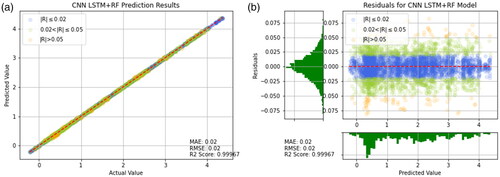
An additional validation was conducted in this study by using a machine tool from National Chung Cheng University. Temperature sensors were placed around the spindle and machine casting as shown in Figure 24. The purpose of the experiment was to verify the effectiveness of the prediction model in other machine tools. The experimental results showed that the proposed model has good predictive ability. As observed in Figure 25, the prediction error was approximately between +0.075 and −0.075. The MAE and RMSE values were both 0.02, and the R² value was 0.99967. The reason for the better performance is that the data was collected in a laboratory with a constant temperature of 20 °C, resulting in less external interference and better prediction accuracy. It can be concluded that the method proposed in this study can be applied to other machine tools and has good predictive ability.

Figure 24. Verification of the sensor installation location on the machining center.

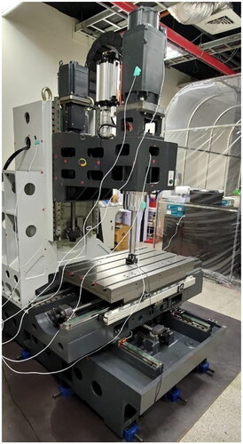
Figure 25. Prediction results of CNN-LSTM for other machining center. (a) Prediction result (b) Prediction error.

However, the model trained in this study is more suitable for a single machine tool and not suitable for multiple machine tools sharing one trained model. This is because the mechanical structure of each machine tool and the temperature of the experimental field can greatly affect the results. Nevertheless, as long as the machine tool is operating normally, the user can immediately collect data and train the prediction model. This approach can save a lot of processing costs during manufacturing.

6. Conclusion and future works

Machining industry has been constantly improving to pursue higher efficiency, higher precision and more energy saving. In the industries, a machine tool must be idling for a period of time before machining, so that its internal structure can achieve a steady state, ready for following machining accordingly. Without such idling stage, the processing precision and quality of the finished products will be degraded due to various errors. In this study, it is intended to address the thermal error, nonlinear, difficult to predict, and needed to be settled urgently in the modern industry. With many literatures, there are many methods proposed to reduce thermal errors by finite elements or artificial technologies. In particular, with the development of science and technology, the computing ability of computers are dramatically enhanced, making artificial technology to be a tool available for research applications in recent years. Therefore, in this paper, it proposes a method of multi-model transfer learning for building better prediction models.

With a combination of this algorithm and the machine tool, machine tool can operate for processing immediately without any warm up, and can make thermal compensation automatically without shutdown or manual measurement, thereby improving the processing accuracy, efficiency as well saving energy, extremely beneficial for the development of future intelligent machine tools.

Disclosure statement

No potential conflict of interest was reported by the author(s).

Additional information

Funding

This work was supported by the National Science and Technology Council, Taiwan, under Grants NSTC 111-2218-E-194-007, NSTC 112-2218-E-194-006, MOST 111-2823-8-194-002, and MOST 111-2221-E-194-052. This work was financially partially supported by the Advanced Institute of Manufacturing with High-tech Innovations (AIM-HI) from The Featured Areas Research Center Program within the framework of the Higher Education Sprout Project by the Ministry of Education (MOE) in Taiwan.

Appendix

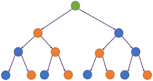
Decision Tree (DT)^[12] is one of the supervised learning algorithms shown in Figure 26, which is further divided into classification tree, regression tree, Classification And Regression Trees (CART), etc. Regression tree is often used to address regression problems, while classification tree is often used to address classification problems. In this study, regression tree is chosen to deal with thermal error prediction. Decision tree is a decision-making tool with tree-like structure, including multiple nodes and branches. Starting from the root node, samples are tested by specific features and assigned to next sub-node according to calculation result. Repeating similar procedures, samples will be transferred to the leaf nodes eventually. Here at leaf nodes, those average values calculated are called predicted values. During predictions in this study, the maximum depth of the tree is set to 3, which better prediction results are achievable.

Figure 26. Architecture diagram of decision tree algorithm.

Random Forest (RF)^[13,14] is an improved regression decision tree algorithm as shown in Figure 27. It basically combines multiple CART trees (Classification And Regression Trees, CART) ^[15] and carries out a combined learning with Bagging algorithm and Regression decision tree algorithm. During creating a CART, it selects variables for splitting randomly, and keeps former procedure until only one sample parameter left after classification at the final node. As a result, decision trees are differentiated from each other, it means that each tree can make its own prediction through split process of each node from top to down and generate predicted output evenly. Comparing with regression decision trees, RF not only improves its own accuracy, but also addresses overfitting issue. In this study, the number of forest trees is set to 1000, and the maximum depth of trees is set to 12.

Figure 27. Architecture diagram of random forest algorithm.

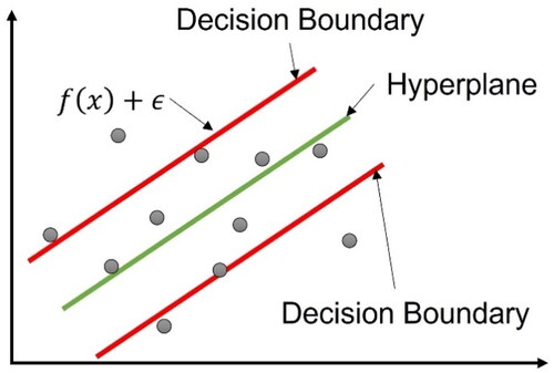
Support Vector Regression (SVR)^[16] as shown in Figure 28 is derived from Support Vector Machine (SVM). SVM is one kind of supervised learning algorithms, which is intended to define the Decision Boundary in space, to find out data points of the Hyperplane, and further to separate and classify two different datasets. The difference between SVR and SVM is that a loss function $\epsilon$ is added to the decision boundary of SVR. Therefore, it allows the error $\epsilon$ between model output and the actual value, and the loss will be calculated only when the error over $\epsilon .$ This algorithm is often used for applications like nonlinear regression predictions, time series predictions. When using this algorithm, it shall be considered to set the penalty function. A penalty method replaces a constrained optimization problem by a series of unconstrained problems which are composed of the original problem, the penalty function and the penalty factor. And it is intended to find out the optimal solution by setting the penalty factor. If the factor is set to a larger value, the penalty for misclassifying samples will be greater. As a result, it may cause overfitting if too large value set. In this study, the penalty function C is set to 1.0, and the kernel of SVR is Radial Basis Function (RBF), which is a polynomial kernel function.

Figure 28. Architecture diagram of support vector regression algorithm.

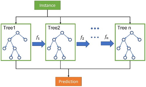
Extreme Gradient Boosting is abbreviated to XGBoost^[17,18] which is a popular algorithm based on Gradient Boosting as shown in Figure 29 in recent years. It applies some new techniques but also keeps some features on Gradient Boosting, so that all trees are related to each other. It is intended to continuously improve and enhance the ability of weak classifiers, and also samples randomly by features, similar technique like Random Forest. In addition, it selects features randomly during forming a tree, so that there will not be all features chosen for making decision in next tree formation every time. Further, in order to fit the training data during model training, there may be many polynomial functions of high degree generated, which causes interference and overfitting due to excessive noise. Therefore, in order to control the complexity of the model, L1/L2 regularization is applied on the loss function to make its curve smoother, thereby improving ability of noise resistance. Finally, all classifiers are combined to form a strong classifier, so that the predictive ability of the whole model is further improved.

Figure 29. Architecture diagram of XGBoost algorithm.

References

- Liu, Y.; Wang, X.; Zhu, X.; Zhai, Y. Thermal error analysis of spindle based on temperature-deformation model. In 2020 4th International Conference on Robotics and Automation Sciences. ICRAS 2020; IEEE: Wuhan, China, 2020; pp. 101–105. DOI: 10.1109/ICRAS49812.2020.9135054.
- Li, H.; Zhang, A.; Pei, X. Research on thermal error of CNC machine tool based on DBSCAN clustering and BP neural network algorithm. In Proceedings of the 2019 IEEE International Conference of Intelligent Applied Systems on Engineering. ICIASE 2019, No. 100; IEEE: Fuzhou, China, 2019. pp. 294–296. DOI: 10.1109/ICIASE45644.2019.9074094.
- Qijun, X.; Zhonghui, L. Intelligent modeling and thermal error test for spindle of high speed CNC machine tools. In Proceedings of the 13th IEEE Conference on Industrial Electronics and Applications. ICIEA 2018; IEEE: Wuhan, China, 2018; pp. 1972–1975. DOI: 10.1109/ICIEA.2018.8398032.
- Fujishima, M.; Narimatsu, K.; Irino, N.; Mori, M.; Ibaraki, S. Adaptive thermal displacement compensation method based on deep learning. CIRP J. Manuf. Sci. Technol. 2019, 25, 22–25. DOI: 10.1016/j.cirpj.2019.04.002.
- Ergen, T. Unsupervised anomaly detection with spark - MapR. IEEE Trans. Neural Networks Learn. Syst. 2020, 31, 1–15.
- Jiao, R.; Zhang, T.; Jiang, Y.; He, H. Short-term non-residential load forecasting based on multiple sequences LSTM recurrent neural network. IEEE Access 2018, 6, 59438–59448. DOI: 10.1109/ACCESS.2018.2873712.
- Xie, J.; Sun, W. A transfer and deep learning-based method for online frequency stability assessment and control. IEEE Access 2021, 9, 75712–75721. DOI: 10.1109/ACCESS.2021.3082001.
- Maeda, K. Speed-up of object detection neural network with GPU Takuya Fukagai Koichi Shirahata Yasumoto Tomita Atsushi Ike Fujitsu Laboratories Limited Fujitsu Software Technologies Limited. In 2018 25th IEEE International Conference on Image Processing. IEEE: Athens, Greece, 2018; pp. 301–305.
- Liu, X.; Qiao, Q.; Dong, B.; Liu, W.; Xu, C.; Xu, S.; Zhou, G. MEMS enabled suspended silicon waveguide platform for long-wave infrared modulation applications. Int. J. Optomechatronics 2022, 16, 42–57. DOI: 10.1080/15599612.2022.2137608.
- Wong, T.-T.; Yeh, P.-Y. Reliable accuracy estimates from K-Fold cross validation. IEEE Trans. Knowl. Data Eng. 2020, 32, 1586–1594. DOI: 10.1109/TKDE.2019.2912815.
- Zhou, G.; Lim, Z. H.; Qi, Y.; Chau, F. S.; Zhou, G. MEMS gratings and their applications. Int. J. Optomechatronics 2021, 15, 61–86. DOI: 10.1080/15599612.2021.1892248.
- Shin, H.; Kang, M.; Lee, S. Mechanism of peripheral nerve modulation and recent applications. Int. J. Optomechatronics 2021, 15, 182–198. DOI: 10.1080/15599612.2021.1978601.
- Chen, J.; Feng, X.; Xiao, S. An iterative method for leakage zone identification in water distribution networks based on machine learning. Struct. Heal. Monit. 2021, 20, 1938–1956. DOI: 10.1177/1475921720950470.
- Prihatno, A. T.; Nurcahyanto, H.; Jang, Y. M. Predictive maintenance of relative humidity using random forest method. In 2021 International Conference on Artificial Intelligence in Information and Communication (ICAIIC); IEEE: Jeju Island, Korea, 2021; pp. 497–499. DOI: 10.1109/ICAIIC51459.2021.9415213.
- Pathak, S.; Mishra, I.; Swetapadma, A. An assessment of decision tree based classification and regression algorithms. In 2018 3rd International Conference on Inventive Computation Technologies (ICICT); IEEE: Coimbatore, India, 2018; pp. 92–95. DOI: 10.1109/ICICT43934.2018.9034296.
- Ren, Q.; Li, M.; Bai, S.; Shen, Y. A multiple-point monitoring model for concrete dam displacements based on correlated multiple-output support vector regression. Struct. Heal. Monit. 2022, 21, 2768–2785. DOI: 10.1177/14759217211069639.
- Wang, S.; Zhong, L.; Niu, Y.; Liu, S.; Wang, S.; Li, K.; Wang, L.; Barton, D. Prediction of frictional braking noise based on brake dynamometer test and artificial intelligent algorithms. Proc. Inst. Mech. Eng. Part D J. Automob. Eng. 2022, 236, 2681–2695. DOI: 10.1177/09544070211062276.
- Preventive control for power system transient security based on XGBoost and DCOPF with consideration of model interpretability. CSEE J. Power Energy Syst. 2020, 7, 279–294 . DOI: 10.17775/CSEEJPES.2020.04780.
- Forouzandeh Shahraki, A.; Al-Dahidi, S.; Rahim Taleqani, A.; Yadav, O. P. Using LSTM neural network to predict remaining useful life of electrolytic capacitors in dynamic operating conditions. Proc. Inst. Mech. Eng. Part O J. Risk Reliab. 2023, 237, 16–28. DOI: 10.1177/1748006X221087503.
- Li, S.; Gu, C.; Li, J.; Wang, H.; Yang, Q. Boosting grid efficiency and resiliency by releasing V2G potentiality through a novel rolling prediction-decision framework and deep-LSTM algorithm. IEEE Syst. J. 2021, 15, 2562–2570. DOI: 10.1109/JSYST.2020.3001630.
- Liu, C.; Ma, J.; Qiu, L.; Fang, Y.; Zhang, J. A torque estimation scheme for induction motor based on GRU and a two-step training process. In 23rd International Conference on Electrical Machines and Systems. ICEMS 2020, No. 1; IEEE: Hamamatsu, Japan, 2020; pp. 1194–1198. DOI: 10.23919/ICEMS50442.2020.9290910.
- Sun, X.; Xu, H.; Dong, Z.; Shi, L.; Liu, Q.; Li, J.; Li, T.; Fan, S.; Wang, Y. CapsGaNet: deep neural network based on capsule and GRU for human activity recognition. IEEE Syst. J. 2022, 16, 5845–5855. DOI: 10.1109/JSYST.2022.3153503.
- Kumar, S. D.; Subha, D. P. Prediction of depression from EEG signal using long short term memory (LSTM). In Proceedings of the International Conference on Trends in Electronics and Informatics, ICOEI 2019, 2019–April (ICOEI), IEEE: Tirunelveli, India, 2019; pp. 1248–1253. DOI: 10.1109/icoei.2019.8862560.
- Zhou, X.; Shi, J.; Gong, K.; Zhu, C.; Hua, J.; Xu, J. A novel quench detection method based on CNN-LSTM model. IEEE Trans. Appl. Supercond. 2021, 31, 1–5. DOI: 10.1109/TASC.2021.3070735.
- Poudyal, A.; Tamrakar, U.; Trevizan, R. D.; Fourney, R.; Tonkoski, R.; Hansen, T. M. Multiarea inertia estimation using convolutional neural networks and federated learning. IEEE Syst. J. 2022, 16, 6401–6412. DOI: 10.1109/JSYST.2021.3134599.
- Sarp, A. O.; Menguc, E. C.; Peker, M.; Guvenc, B. C. Data-adaptive censoring for short-term wind speed predictors based on MLP, RNN, and SVM. IEEE Syst. J. 2022, 16,–3625–3634. DOI: 10.1109/JSYST.2022.3150749.
- Liu, X.; Yu, W.; Liang, F.; Griffith, D.; Golmie, N. Toward deep transfer learning in industrial internet of things. IEEE Internet Things J 2021, 8, 12163–12175. DOI: 10.1109/JIOT.2021.3062482.
- Sun, G.; Ayepah-Mensah, D.; Xu, R.; Agbesi, V. K.; Liu, G.; Jiang, W. Transfer learning for autonomous cell activation based on relational reinforcement learning with adaptive reward. IEEE Syst. J. 2022, 16, 1044–1055. DOI: 10.1109/JSYST.2021.3059892.
- Zana, R. R.; Zelei, A. Feedback motion control of a spatial double pendulum manipulator relying on swept laser based pose estimation. Int. J. Optomechatronics 2021, 15, 32–60. DOI: 10.1080/15599612.2021.1890284.
- Liang, J.-B.; Lin, W.-P.; Wu, R.; Chen, C. Correlation of accommodation and lens location with higher-order aberrations and axial length elongation during orthokeratology lens wear. Int. J. Optomechatronics 2021, 15, 1–9. DOI: 10.1080/15599612.2020.1857889.
Appendix
Decision Tree (DT)[Citation12] is one of the supervised learning algorithms shown in , which is further divided into classification tree, regression tree, Classification And Regression Trees (CART), etc. Regression tree is often used to address regression problems, while classification tree is often used to address classification problems. In this study, regression tree is chosen to deal with thermal error prediction. Decision tree is a decision-making tool with tree-like structure, including multiple nodes and branches. Starting from the root node, samples are tested by specific features and assigned to next sub-node according to calculation result. Repeating similar procedures, samples will be transferred to the leaf nodes eventually. Here at leaf nodes, those average values calculated are called predicted values. During predictions in this study, the maximum depth of the tree is set to 3, which better prediction results are achievable.