Response to Williams (2010) on Gard (2009): Comparison of spawning habitat predictions of PHABSIM and River2D models

Williams (2010) raises a number of interesting points with regard to the testing of instream flow models. Before responding to the critique and suggestions of Williams (2010), I note several inaccuracies in Williams (2010). River2D does not divide the study area into cells. River2D calculates depths and velocities at nodes of the triangulated irregular network, and then interpolates between the surrounding nodes to calculate depths and velocities at any given location. There are two types of two-dimensional (2D) hydraulic models – finite element and finite difference (Steffler and Blackburn 2002). River2D is a finite-element model. It would be accurate to say that finite difference 2D models divide the study area into cells. Gard (2009) used the one-dimensional model throughout the sites, since the entire area of all of the sites did not have transverse flow or other complex flow patterns. There definitely are other portions of the Sacramento, American, and Merced Rivers where PHABSIM could not be used due to transverse flow or other complex flow patterns, but they were not in the 13 study sites addressed by Gard (2009). The weighted useable area presented in Gard (2009) is not normalized by channel length. However, Williams (2010) is correct that usually weighted usable area (WUA) is normalized by channel length. The comparison of measured and simulated velocities in Gard (2009) is not for redd locations, but rather for the sites overall – this is for validation of the hydraulic model, before any consideration of biology.

In the interest of brevity, my responses to Williams (2010) will focus on the American River as an example. We are exploring a number of biological verification tests, in addition to the Mann–Whitney tests used in Gard (2009). A key aspect of whatever test is used is having a quantitative measure to conclude whether or not the combined hydraulic and biological models have been verified. Box plots, as shown for the American River data (Figure 1), do not appear to be an effective means to present the magnitude of differences and precision of estimates. Rather, I suggest that histograms of combined suitability (Figure 2) are a better means to display effects and precision. Although the histograms provide a good visual comparison, they still do not provide a quantitative measure to conclude whether or not the combined hydraulic and biological models have been verified. Gard (2009) used statistical tests of combined suitability and WUA curves because, right or wrong, statistical tests are the norm for publications in the scientific literature (Johnson 1999). Given the hypothesis to be tested, the combined suitability index (CSI) of occupied locations are greater than the CSI of unoccupied locations; a Mann–Whitney U-test is a logical choice, given that CSI is not normally distributed (Figure 2). The rationale for using a Kolmogorov–Smirnov test is that it is a logical choice to test the hypothesis: the flow-habitat relationships predicted by PHABSIM and River2D have different shapes. I agree with Williams (2010) that it is difficult to determine what the appropriate degrees of freedom is for the Kolmogorov–Smirnov test, as used in Gard (2009). It would be good to have a quantitative objective method to determine how many of the 55 comparisons of PHABSIM and River2D flow-habitat relationships have practical differences, such as resulting in different flow management decisions, but I am not aware of any such method.

Figure 1 Box plots of American River fall-run Chinook salmon spawning CSI for occupied locations calculated from measured depths, velocities, and substrates, and for occupied and unoccupied locations simulated by River2D (2D) and PHABSIM. Depths, velocities, and substrate sizes were not measured at unoccupied locations

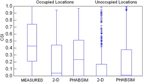
Figure 2 Frequency distributions of American River fall-run Chinook salmon spawning CSI for occupied locations calculated from measured depths, velocities, and substrates, and for occupied and unoccupied locations simulated by River2D (2D) and PHABSIM

Scatter plots of measured versus predicted depths, velocities, and substrate sizes at redd locations (Figures 3–5) indicate that most of the errors in redd predictions can be attributed to the hydraulic models. Although River2D performed somewhat better (correlations of 0.23 and 0.46 between, respectively, measured and predicted velocities and depth, and 26% of redds with the same simulated and measured substrate size) than PHABSIM (correlations of −0.008 and 0.36 between, respectively, measured and predicted velocities and depth, and 19% of redds with the same simulated and measured substrate size), both hydraulic models had substantial errors. It should be noted that the River2D simulations in Gard (2009) were the first River2D models we had developed, and our more recent River2D modelling has had much lower errors (with correlations between measured and simulated velocities ranging from 0.64 to 0.82), principally due to a higher density of bed topography data used to develop the River2D models (typically at least 40 points/100 m², versus the density of 2.65 points/100 m² used in Gard (2009)).

Figure 3 Scatterplots of American River fall-run Chinook salmon redd depths simulated by River2D and PHABSIM versus measured redd depths

Figure 4 Scatterplots of American River fall-run Chinook salmon redd velocities simulated by River2D and PHABSIM versus measured redd velocities

Figure 5 Frequency distribution of American River fall-run Chinook salmon redd substrate sizes simulated by River2D and PHABSIM versus measured redd substrate sizes

The conceptual basis for the habitat suitability criteria (HSC) used in Gard (2009) is given in Gard (1998). Specifically, bioenergetic considerations and physical abilities of adult salmonids will limit the maximum velocity and substrate size used for spawning, and some minimum depth is necessary to physically allow salmonids to spawn (Gard 1998). In contrast, requirements of the developing eggs and larvae for sufficient intragravel velocities will set a lower limit on the velocity and substrate size used for spawning (Gard 1998). The decline in habitat use in deeper water is largely due to low availability of deep waters with suitable velocity and substrate (Gard 1998). The depth criteria in Gard (2009) were developed using the method in Gard (1998) where a series of linear regressions are used to correct habitat use for availability, using data on use and availability (Figure 6). It should be noted that logistic regressions also correct habitat use for availability, and thus typically result in a shift in the habitat suitability criteria, compared with habitat use data. It is the standard practice in instream flow studies to assume that all independent variables are equally significant and to have compound suitability calculated as the product of the habitat suitability index (HSI) of the independent variables (Bovee 1996, p. 120). This assumption has previously been tested and validated in the peer-reviewed literature (Vadas and Orth 2001).

Figure 6 Relations between relative availability and use and depth for the American River. Points are relative use, relative availability, or the ratio of the linearized use to linearized availability for the American River. Lines are the results of the linear regressions of the depth increment versus relative availability and use for the American River. Adapted from Gard (1998)

I agree with Williams (2010) that logistic regression is a superior method for developing suitability criteria. It is well established in the literature (Knapp and Preisler 1999, Parasiewicz 1999, Geist et al. 2000, Guay et al. 2000, Tiffan et al. 2002, McHugh and Budy 2004) that logistic regressions should be used to develop habitat suitability criteria. For example, McHugh and Budy (2004) state (p. 90):

More recently, and based on the early recommendations of Thielke (1985), many researchers have adopted a multivariate logistic regression approach to habitat suitability modeling (Knapp and Preisler 1999, Geist et al. 2000, Guay et al. 2000).

Traditionally, criteria are created from observations of fish use by fitting a nonlinear function to the frequency of habitat use for each variable (depth, velocity, and substrate). The main concern with this technique is the effect of availability of habitat on the observed frequency of habitat use. For example, if a substrate size is relatively rare in a stream, fish will be found primarily not using that substrate size simply because of the rarity of that substrate size, rather than because they are selecting areas without that substrate size. Guay et al. (2000) proposed a modification of this technique where depth, velocity, and substrate data are collected both in locations where redds are present and in locations where redds are absent, and a logistic regression is used to develop the criteria. We have used logistic regressions in more recent studies to develop HSI curves. Logistic regression, versus the standard HSI based solely on habitat use, is primarily useful in streams where habitat availability is limited, and thus is affecting habitat use. Such was not the case in the streams studied here. There were sufficient areas present in these streams of the range of depths, velocities, and substrates used by Chinook salmon for spawning that the salmon were able to select the habitat conditions that they preferred, with the exception of availability of deeper areas, where the methods in Gard (1998) were applied to correct for availability. If there is a relatively uniform distribution of unoccupied depths, velocities, and substrates, as would be the case in these streams, logistic regression and standard HSI based solely on habitat use should give similar results.

I applied the approach advocated by Williams (2010) to the American River CSI data (Figure 7). I was not able to calculate confidence intervals because the occupied locations are all of the occupied locations in the whole study area, so that this is a census, not a sample, at least within the study area. Confidence intervals apply to samples, not complete counts. I was not able to apply this approach to measured data because we did not collect measurements at unoccupied locations. There was no relationship between combined suitability and the percentage of occupied locations for PHABSIM. While the data for suitabilities of 0.2–0.6 approximated a straight line lying on the diagonal for River2D, the data deviated significantly from the diagonal for suitabilities outside this range. I suspect that the deviation for suitabilities of 0–0.2 are attributable to errors in the hydraulic model, where simulated depths, velocities and/or substrate sizes produced lower suitabilities than would be expected from the measured data. In contrast, I suspect the deviation for suitabilities of 0.6–1 are attributable to low sample sizes – for example, the percentage of occupied locations for the 0.9–1 suitability increment was based on only four occupied and six unoccupied locations. I suspect that this approach did not work in this case because the suggested method is not very powerful for small sample sizes – based on the cases I looked at, it appears that one needs at least 150 observations to develop a meaningful test of the relationship between combined suitability and percent occupied locations. With less than 150 redds, there would be an average of less than 15 redds in each of the combined suitability bins – this probably results in type II errors, since random variation could result, for example, in a bin with no redds, which would have a large effect on the analysis. The suggested approach and the U-test are looking at similar relationships: in the suggested approach, the hypothesis tested is that there is a positive relationship between the percentage of occupied locations and combined suitability, while in the U-test the hypothesis tested is that the combined suitability of occupied locations is greater than unoccupied locations. So in both cases what is being examined is the relationship between use and availability – i.e. are fish selecting areas with high suitability. The suggested approach may have other flaws: if the availability of high CSI areas is extremely limited, just by chance there might not be any redds in areas with high CSI.

Figure 7 Plots of percentage occupied locations versus CSI simulated by River2D and PHABSIM for American River fall-run Chinook salmon spawning. Plots of percentage occupied locations based on measured data cannot be prepared since measurements were not made at unoccupied locations

Acknowledgements

Thanks to S. Gallagher and J. Williams for providing useful reviews that improved the original manuscript. The studies were funded by the Central Valley Project Improvement Act (Title XXXIV of P.L. 102-575).

References

- Bovee , K. D. 1996 . The complete IFIM: a coursebook for IF 250 , Edited by: Bovee , K. D. Fort Collins, CO : US Geological Survey .
- Gard , M. 1998 . Technique for adjusting spawning depth habitat utilization curves for availability . Rivers , 6 ( 2 ) : 94 – 102 .
- Gard , M. 2009 . Comparison of spawning habitat predictions of PHABSIM and River2D models . International Journal of River Basin Management , 7 ( 1 ) : 55 – 71 .
- Geist , D. R. 2000 . Suitability criteria analyzed at the spatial scale of redd clusters improved estimates of fall Chinook salmon (Oncorhynchus tshawytscha) spawning habitat use in the Hanford Reach, Columbia River . Canadian Journal of Fisheries and Aquatic Sciences , 57 ( 8 ) : 1636 – 1646 .
- Guay , J. C. 2000 . Development and validation of numerical habitat models for juveniles of Atlantic salmon (Salmo salar) . Canadian Journal of Fisheries and Aquatic Sciences , 57 ( 10 ) : 2065 – 2075 .
- Johnson , D. H. 1999 . The insignificance of statistical significance testing . Jounal of Wildlife Management , 63 ( 3 ) : 763 – 772 .
- Knapp , R. A. and Preisler , H. K. 1999 . Is it possible to predict habitat use by spawning salmonids? A test using California golden trout (Oncorhynchus mykiss aguabonita) . Canadian Journal of Fisheries and Aquatic Sciences , 56 ( 9 ) : 1576 – 1584 .
- McHugh , P. and Budy , P. 2004 . Patterns of spawning habitat selection and suitability for two populations of spring Chinook salmon, with an evaluation of generic verses site-specific suitability criteria . Transactions of the American Fisheries Society , 133 ( 1 ) : 89 – 97 .
- Parasiewicz , P. A hybrid model – assessment of physical habitat conditions combining various modeling tools . Proceedings of the third international symposium on ecohydraulics . Salt Lake City, Utah.
- Steffler , P. and Blackburn , J. 2002 . “ River2D: two-dimensional depth averaged model of river hydrodynamics and fish habitat ” . In Introduction to depth averaged modeling and user's manual , Edmonton, Alberta : University of Alberta . Available from: http://www.river2d.ualberta.ca/download.htm (Accessed 9 March 2010)
- Thielke , J. A logistic regression approach for developing suitability-of-use functions for fish habitat . Proceedings of the symposium on small hydropower and fisheries . Edited by: Olson , F. W. , White , R. G. and Hamre , R. H. pp. 32 – 38 . Bethesda, MD : American Fisheries Society, Western Division and Bioengineering Section .
- Tiffan , K. E. , Garland , R. D. and Rondorf , D. W. 2002 . Quantifying flow-dependent changes in subyearling fall Chinook salmon rearing habitat using two-dimensional spatially explicit modeling . North American Journal of Fisheries Management , 22 ( 3 ) : 713 – 726 .
- Vadas , R. L. and Orth , D. J. 2001 . Formulation of habitat suitability models for stream fish guilds: do the standard methods work? Transactions of the American Fisheries Society . 130 ( 2 ) : 217 – 235 .
- Williams , J. G. 2010 . Comment on Gard (2009): Comparison of spawning habitat predictions of PHABSIM and River2D models . International Journal of River Basin Management , 8 (1), 117–119