3D simulation of flow around a single spur dike with free-surface flow

Abstract

In the present study, flow patterns around a single spur dike (also termed a groyne) with free-surface flow was simulated using a numerical model known as Fluent. The model solved the fully three-dimensional, Reynolds-averaged Navier–Stokes equation to predict flow near the structure where three-dimensional flow is dominant. To treat the complex free-surface flow, the volume of fluid method with geometric reconstruction scheme was applied and turbulence was simulated using standard equations. In this research work, both a structured and an unstructured mesh were used and the density of the mesh spacing was selected the highest near the walls and also free surface to obtain more accurate results. Comparison of free surface and velocities of 3D model showed good agreement with three experimental flume data obtained by other researchers. The reattachment length for various conditions was computed using the numerical results and flow pattern was presented for repelling, attracting and vertical spur dikes together. Also, bed-shear stress distribution was presented and the effects of flow discharge and the length and angle of the spur dike upon the bed shear-stress distribution were evaluated.

Keywords:

• Spur dike
• simulation
• numerical model
• Fluent
• k − ω
• free surface
• VOF
• shear stress

1 Introduction

Spur dikes (also known as groynes) are often used in river engineering for navigation or bank support such as confining flow through a bridge, as well as in coastal engineering for bank or beach protection. Construction of a spur dike aligned with the river flow direction decreases the width of river and causes flow separation around the spur dike and recirculation of downstream streamlines. Due to contraction of streamlines and increasing velocity, the river bed is subject to extensive scour and a scour hole will likely form. Local scour around spur dikes is a problem and numerous researchers are investigating this phenomenon because of the potential for damaging erosion and costly structural failures creating hazards to the public. Chen and Li (1989) simulated the flow field and distribution of turbulent kinetic energy and its dissipation rate by using a depth-average two-dimensional (2D) turbulent modelling with equations. Tingsanchali and Maheswaran (1990) used a 2D depth-averaged model, incorporating a correction factor to improve the computed bed-shear stress. Molls et al. (1995) developed 1D and 2D models to simulate the flow characteristics of spur dike. Mayerle et al. (1995) adopted static pressure to simulate the flow around spur dike and the effect of the side-wall boundary condition on stream velocities using a 3D model. They assumed a hydrostatic-pressure distribution and suggested that it may explain the discrepancies of the flow patterns in the vicinity of the spur dike. Zhou (2001) developed a large eddy simulation (LES) model to describe the velocity field around a spur dike. Ettema and Muste (2004) studied a series of flume experiments and determined scale effects in small-scale models of flow around a single spur dike placed in a channel whose bed is fixed and flat. Peng (2004) summarized the results of experimental and numerical simulation on a spur dike and analysed the structure of flow field and local scour around a spur dike. Uijttewaal (2005) investigated the effects of various spur-dike shapes on the flow in a spur-dike field in a physical model of a schematized river reach, geometrically scaled at 1:40. These experiments showed that the turbulence properties near and downstream from a spur dike and hence scour can be minimized by changing the permeability and slope of the upstream end of a spur dike. It was also observed that for submerged conditions, the flow becomes more complex and locally dominated by 3D effects, which make it difficult to use 2D depth-averaged numerical models or 3D models using a coarse resolution in the vertical direction. Xuelin et al. (2006) used LES to model the three-dimensional flows around a non-submerged spur dike and analysed vortex flows downstream from the spur dike. Xuelin (2007) also investigated flow patterns around a non-submerged spur dike in a physical model of the approach to the navigation channel of the Three Gorges Project in China. The finite-volume method (FVM) was used to discretize the governing equations together with a staggered-grid system (Versteeg and Malalasekera 1995). The computational results were in a fairly good agreement with the experimental data. MacCoy et al. (2008) studied the flow hydrodynamics in a straight open channel containing a multiple-embayment spur-dike field on one of its sides numerically using large-eddy simulation and analysed mixing-layer eddies around the spur dike. Although to date (2009) various researchers have conducted studies on this phenomenon, few of evaluated models incorporated fully 3D turbulent modelling and free-surface flow. In this research, flow around a spur dike was simulated with a fully 3D model and volume of fluid (VOF) method was applied to simulate free-surface flow. Also, we evaluated the effects of various parameters on the flow pattern and bed stress in the vicinity of the spur dike was studied using numerical results.

2.  Experimental data collected

To evaluate the model's applicability, three experimental cases were selected. The test cases included three fixed-bed cases. The first experimental test was conducted in a flume with dimensions that were 0.4 m wide, 0.4 m deep, and about 18 m in length that was designed/built/operated by Zhou et al. (2004). The experiment observational zone was 2.0 m long and the spur dike was rectangular with 0.1 m long, 0.05 m high, and 0.015 m wide and was installed in the middle of the test zone. In this test, the spur dike was placed at a 60° angle towards the upstream and was submerged in the water. The flume discharge was 0.015 m³/s with a flow depth 0.1 m and the bed slope had a gradient of 0.0004 m/m.

In the second case, flume experiments were conducted in a channel 8.0 m in length, 0.3 m in width by Tominaga and Chiba (1996). The rectangular spur dike was 0.15 m long, 0.05 m high, and 0.03 m wide and was located at a distance from x  =  4.0 m to x  =  4.03 m and was installed in the straight channel with a fixed flat bed. In this physical model, the measured discharge was 0.0036 m³/s, flow depth 0.09 m, bed slope was 0 m/m, and the angle of spur dike was 90° in the left-side bank of the straight channel, and the spur dike was below the water surface.

For the third case, tests were conducted in a straight rectangular flume 37 m long, 0.9 m wide, and 0.3 m height (provide the height and slope of the flume) by Nawachukwu (1979). The spur dike consisted of an aluminium plate (3 mm thick, 152 mm long, 300 mm height) and projected well above the water surface. The velocities were measured from 0.92 m upstream from the spur dike to 1.22 m downstream from the spur dike using a pitot-static tube in the regions where the flow was undisturbed and a three-tube yaw probe in the skewed regions. These three cases of flume experiments were used to evaluate the 3D numerical model. The geometric parameters of these models were presented in Table 1.

Table 1 Geometric parameters of experimental models used in the presented paper

Model	Length (m)	Width (m)	Flow depth (cm)	Angle towards upstream	Location of spur dike (m)	Dimensions of spur dike
						Length (m)	Thickness (m)	Height (m)
Zhou et al. (2000)	3.5	0.4	10	60	x  =  1	0.1	0.015	0.05
Tominaga et al. (1996)	8	0.3	9	0	x  =  4	0.15	0.03	0.05
Nawachukwu (1979)	12	0.9	30	0	x  =  3	0.152	0.003	0.3

3 Numerical modelling

Fluent computational fluid dynamics (CFD) code was used for 3D numerical modelling. Numerical modelling involves the solution of the Navier–Stokes equations, which are based on the assumptions of conservation of mass and momentum within a moving fluid. The conservation of mass is described by the differential equation

In this equation, is velocity and is the density of the fluid.

The momentum equation is described as shown below:

where p is the pressure, the velocity, and g is gravity. , where is viscosity of fluid, the turbulence viscosity, and the body force. In this research, the objective was to determine and the standard model was used because of re-circulating flow around the spur dike: , where is an empirical constant equal to 0.09, and k and ω are obtained from the following transport equations (Launder and Spalding 1974):

where represents the generation of turbulent kinetic energy due to the mean velocity gradients, and are constants, and are the turbulent Prandtl numbers for and , respectively. Standard constants of mode are listed in Table 2, and were used in the model.

Table 2 The standard turbulence model constants

2	2	0.09	0.555	0.8333

To represent the sharp interface between the air and water, the VOF method of Hirt and Nichols (1981) is used. In this approach, the interface is tracked by introducing the volume fraction for the ith phase – that is, the fraction of the volume of a cell occupied by that phase. When modelling the free surface between water and air, a transport equation is solved for the water phase:

which holds in the absence of any inter-phase mass transfer and where is the volume fraction of water. Only one such transport equation needs to be solved since the volume fraction of the other phase can be inferred from the constraint , where is the volume fraction of air. The FVM is used to solve the above equations and relies on the flow domain being divided into a grid consisting of a large number of cells. In each cell, if it contains only water, then ; if none, then . For cells that span the interface between the air and water, . Thus, it can be assumed that the free surface is on the volume fraction of 0.5. Also Dargahi (2006) used the volume fraction of 0.5 to define the free surface. The fluid properties in each cell are adjusted according to the local volume fraction; for example, the density in each cell is , with a similar expression for the dynamic viscosity, . Various algorithms have been developed to sharpen the interface between two phases because the interface tends to be smeared if Eq. 5 is used alone. In the present work, the geometric reconstruction method of Young (1982) was employed. This scheme uses a linear interpolation in tracing the interface of two phases and is more accurate than the other schemes.

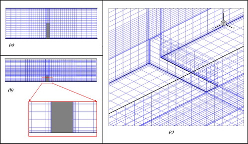
In the present research, both a structured and an unstructured mesh were used. An unstructured mesh was used around the inclined part of the spur dike because of complex geometry, and a structural mesh was used for the vertical spur dike. Figure 1 shows the mesh on the wall boundaries for the experimental model of Tominaga and Chiba (1996). The area around the spur dike used a finer mesh than the other region. The number of mesh in vertical view was increased near the free surface to trace more accurately the free surface. Also, in boundary layers a more dense mesh is used to consider the viscous flow in sublayers. The first grid surface off the solid boundaries was at , which ensures that the first grid surface off the wall is located almost every where at ( ) and that at least two grid surfaces are located within the laminar sublayer ( ), where is the distance of first grid from the solid wall, is wall shear stress, and is kinetic viscosity.

Figure 1 Computational grid in the vicinity of a spur dike: (a) plan view, (b) vertical view and (c) 3D view

Boundary conditions were as follows (Figure 2).

Figure 2 Domain of solutions and boundaries for a spur dike

Two different inlets were needed to define the water flow (Inlet I) and air flow (Inlet II) in the model domain. These inlets were defined as stream-wise velocity inlets that require the values of velocity. To estimate the effect of wall on the flow, empirical wall functions known as standard wall functions (Launder and Spalding 1974) were used. The turbulence model was used with standard-wall functions. The has advantages when there is strong recirculation flow such as in the case of spur dikes. The upper boundary above the air phase was specified as a symmetry condition, which enforces a zero normal velocity and a zero shear stress.

To complete the description of the CFD modelling, the PRESTO pressure discretization scheme was used because this scheme was showed the best convergence in this model. Other researchers also used this scheme in their studies, such as Dargahi (2006) and Hargreaves et al. (2007). The PISO pressure-velocity coupling algorithm was used purely because it is designed specifically for transient simulations.

The unsteady, free-surface calculations required fine grid spacing and small initial time steps. The grid spacing used was adequate for solution convergence and showed good agreement with the experimental results. A time step equal to 0.01 or 0.001 was selected. During the 3D model runs, solution convergence and the water-surface profiles were monitored. Convergence was reached when the normalized residual of each variable was on the order of 1 × 10⁻³. The free surface was defined by a value of VOF = 0.5, which is a common practice for volume fraction results (Fluent Manual 2005, Dargahi 2006). After the convergence of the numerical solution, in order to obtain more accurate results, again mesh was refined according to gradients of two phases and velocities and the model was run. The final number of mesh in various conditions changed in the ranges 182094–329969 cells. A sensitivity analysis was used and number of mesh increased two times that showed the results of model were valid.

Computations were conducted using a Pentium IV system with an AMD 3800₊ processor. Each run of the numerical model took 6–18 h depending on spur dike dimensions, mesh numbers, time step, and flow characteristics.

4 Verification

Before employing the numerical model to study the flow pattern around the spur dike, it was necessary to ensure the accuracy of the numerical model. For this purpose, experimental cases mentioned in upper section were employed. To evaluate the free surface, the first case was selected regarding the available flume data.

To assess the flume and model water-surface profiles, one cross-section (x = 1.10 m) and one longitudinal section (y = 0.04 m) were selected. The compared results are shown in Figures 3 and 4. For this model configuration, computed error at the cross-section was 2% and the longitudinal error was 1.8%.

Figure 3 Comparison of flume and modelled results of free surface flow around a spur dike in experiments of Zhou et al. (2004), (a) at cross-section x  =  1.1 m, (b) at longitudinal section y  =  0.04 m

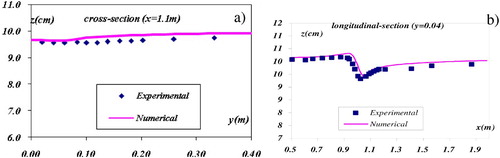
Figure 4 Comparison of numerical model velocities and measured data in flume experiments of Tominaga and Chiba (1996), (a) at dir. 3 and 4, (b) at dir. 1 and 2

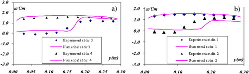
To evaluate the flow domain, the second and third cases were selected regarding the available data. In the second case and for the convenience of comparison, four directions are selected: direction 1, x = 4.0 m, z = 0.07 m; direction 2, x = 4.1 m, z = 0.01 m; direction 3, x = 4.05 m (0.02 m downstream from the spur dike), z = 0.02 m; and direction 4, x = 4.05 m, z = 0.07 m, at zone behind the spur dike. From Figure 4, it can be seen that agreements between the measured and computed velocities are satisfactory. Maximum error (in terms of depth) was observed in directions 2 and 3, which have small depths. For such small depths, the two equation turbulence models cannot predict turbulence precisely due to the existence of a shear layer between the recirculation zones and flow in the downstream direction.

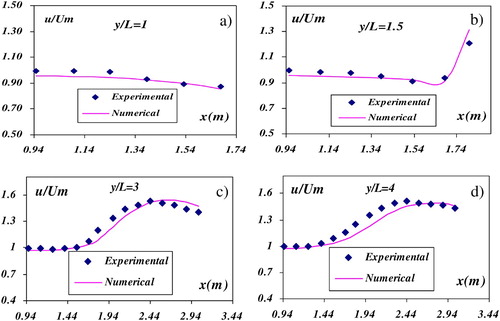
For third case, the modelled results were compared with the flume experimental data obtained by Nawachukwu (1979) shown in Figure 5. The resultant velocity was non-dimensionalized with reference to the mean velocity . The values are plotted at y/L = 1, 1.5, 3 and 4 in the y-direction and from x = 0.92 m to x = 3 m (L is length of groyne). The agreement between the flume and 3D modelled results is satisfactory. In these tests, the measured errors were 2.81%, 3.58%, 3.7%, and 4.15% for y/L = 1, 1.5, 3, and 4, respectively.

Figure 5 Comparison of numerical velocities and measured data in flume experiments of Nawachukwu (1979), (a) at y/L  =  1, (b) y/L  =  1.5, (c) y/L  =  3, (d) y/L  =  4

These results show the accuracy of the numerical model in calculating the flow field around a spur dike. In the next stage, changing various parameters included discharge, length and angle of the spur dike, the 3D numerical model was used to study effect of these parameters on the computed flow field, shear-stress distributions, and the scour location. The design criteria recommended and where is the maximum length of the spur dike, and is the angle of the deviation of the spur dike and ‘w’ is the width of channel. To conform with the criteria above, experimental model of Tominaga and Chiba (1996) was used (because of its small dimensions to shorten time of numerical model runs) for subsequent runs of program. However, the length of the spur dike was selected based on the following criterion: the thickness of the spur dike was selected as 0.1L and its height was selected so that the spur dike was not submerged. The selected lengths of the modelled spur dike were .

5 Analysis of computational results

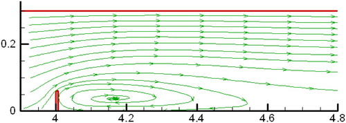
Streamlines of flow around the spur dike near the bed are shown in Figure 6. A circulation zone formed downstream from the spur dike due to the direction of flow by the spur dike and downstream flow separation shown in Figure 6. The reattachment length (l) was computed as for the vertically oriented spur dike, which confirms with experiments obtained for 11.5L by Ouillon and Le Guennec (1996). Near the water surface, streamlines are similar, but the reattachment length decreased because of higher velocities.

Figure 6 Streamlines around a spur dike near the bed

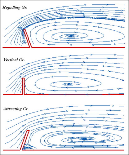
Streamlines also were drawn for repelling and attracting spur dike as shown in Figure 7. It can be seen that for the upstream-oriented spur dike two recirculation zones exist. In this case, a small swirl zone upstream from the spur dike was formed due to flow at the spur dike. For the downstream-oriented spur dike, two downstream recirculation zones were observed. A small swirl zone formed at the attachment point of the spur dike and the wall due to flow paths at the spur dike and reversal of flow direction.

Figure 7 Effect of angle of a spur dike on the flow streamlines

The reattachment length for various runs was calculated and presented in Table 3. , where w is width of the flume, l is reattachment length, h is width of the recirculation zone and is the discharge for the physical model. From this table, one can observe that the effects of the spur-dike angle (for the recommended ranges) and discharge on the length of recirculation zone (reattachment length) are relatively short; however, the length of the spur dike has a considerable effect upon the reattachment length by shortening the length of spur dike by a half, and there was no recirculation in downstream of groyne and only separation is occurred. For a spur dike twice as long, the reattachment length increased more than two times. As listed in Table 3, the angle of spur dike and the discharge have little effect on the width of the recirculation zone, but the length of the spur dike has a great effect on the dimension of the recirculation zone.

Table 3 Reattachment length for various experimental conditions

Case
	11.67	10.33	10.66	5.8325	23.33	9	11.67
	0.095	0.1	0.9	0.10	0.15	0.095	0.095

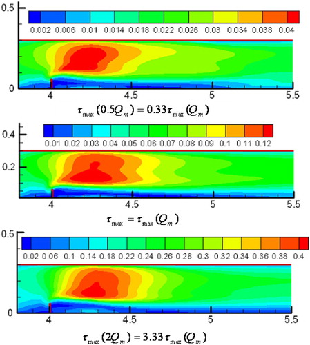
The analysis of the shear-stress field at the channel bed presents a particular interest for studying the sediment transport around a spur dike. The criterion of initial motion of sediment at the streambed is generally estimated using a critical-shear stress threshold (Ouillon and Le Guennec 1996). Potential depositional and erosional zones are estimated from the bed shear-stress values. Downstream from a spur dike in the recirculation zone, shear-stress decreases and deposition occurs. Near the tip of the spur dike, velocity and shear stress increase and bed erodes. The effect of angle and length of a spur dike and discharge on the bed-shear stress are shown in Figures 8 and 9. From Figure 8(a), one can notice that the maximum shear stress in vertical spur dike is higher than for other angles. At a vertical spur dike, velocity gradients near the bed are larger, and therefore, shear stress values are higher. As shown in Figure 8(b) for longer spur dikes, shear stress increased due to increased velocities flowing by spur dikes with smaller widths. Also, larger discharge results in higher velocity around the spur dike and bed-shear stresses increase (Figure 9), and therefore potential erosion downstream from the spur dike increases substantially.

Figure 8 Bed-shear stress: (a) for various angles of spur dikes, (b) for various lengths of spur dikes

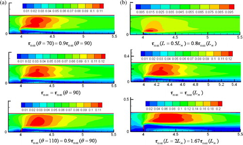
Figure 9 Bed-shear stress for various discharges

6 Conclusions

In this research, flow patterns around spur dikes were studied using a 3D-numerical hydraulic model. The turbulence model with the VOF method was used to simulate fully three-dimensional flows. The numerical modelling uses the Navier–Stokes equations within the flow domain upstream and downstream from a spur dike that used experimental flume data obtained by other researchers. By comparing the 3D model with the flume results, the model was found to produce flow around a spur dike with sufficient accuracy. Then, the effect of varying parameters such as discharge, angle and length of the spur dike upon flow pattern and bed-shear stress results were evaluated. These studies showed that length and width of the recirculation zone (reattachment length) for various angles of the spur dike ( ) are approximately constant. Also, varying the discharge has little effect on the reattachment length, but changing the length of the spur dike has considerable effects on the dimensions of recirculation zone. The maximum bed-shear stress was observed in vertical spur dike rather than for spur dikes oriented upstream or downstream.

Notation

g	=	gravity acceleration
h	=	width of recirculation zone
l	=	reattachment length
L	=	length of spur dike
L m	=	length of spur dike for mean flow
L max	=	maximum length of spure dike
p	=	pressure
Q m	=	water flow discharge for mean flow
u	=	velocity
U m	=	mean velocity
w	=	width of channel
x,y,z	=	Cartesian coordinates

Greek symbols

	=	volume fraction of water
	=	volume fraction of air
	=	kinematics viscosity of water
	=	density of fluid
	=	viscosity of fluid
	=	turbulent viscosity
	=	angle of the deviation of the spure dike
	=	wall shear stress
	=	the distance of first grid from the solid wall

Acknowledgements

The authors thank Robert D. Jarrett, US Geological Survey USGS, for his suggestions in preparation of this manuscript and also reviews.

References

- Chen , N. S. and Li , C. H. 1989 . Numerical solution of the flow around a spur dike with turbulent model . Journal of Nanjing Hydraulic Research Institute , 3 : 11 – 23 .
- Dargahi , B. 2006 . Experimental study and 3D numerical simulations for a free-overflow spillway . Journal of Hydraulic Engineering , 132 ( 9 ) : 899 10.1061/(ASCE), 0733–9429
- Ettema , R. and Muste , M. 2004 . Scale effects in flume experiments on flow around a spur dike in flatbed channel . ASCE, Journal of Hydraulic Engineering , 130 ( 7 ) : 635 – 646 .
- Fluent Manual . 2005 . Manual and user guide of Fluent Software , Fluent Inc .
- Hargreaves , D. M. , Morvan , H. P. and Wright , N. G. 2007 . Validation of the volume of fluid method for free surface calculation: the broad-crested weir . Engineering Applications of Computational Fluid Mechanics , 1 ( 2 ) : 136 – 146 .
- Hirt , C. W. and Nichols , B. D. 1981 . Volume of fluid methods for the dynamics of free boundaries . Journal of Computational Physics , 39 : 201 – 225 .
- Launder , B. E. and Spalding , D. B. 1974 . The numerical computation of turbulent flows . Journal of Computer Methods in Applied Mechanics and Engineering , 3 : 269 – 289 .
- MacCoy , A. , Constantinescu , G. and Weber , J. 2008 . Numerical investigation of flow hydrodynamics in a channel with series of groynes . ASCE, Journal of Hydraulic Engineering , 134 ( 2 ) : 157 – 172 .
- Mayerle , R. , Toro , F. M. and Wang , S. S.Y. 1995 . Verification of a three-dimensional numerical model simulation of the flow in the vicinity of spur dikes . Journal of Hydraulic Research , 33 ( 2 ) : 243 – 256 .
- Molls , T. , Chuadhry , M. H. and Khan , K. W. 1995 . Numerical simulation of two dimensional flow near a spur dike . Journal of Advance in Water Resources , 118 ( 4 ) : 227 – 236 .
- Nawachukwu , B. A. 1979 . Flow and erosion near groyne-like structures , Edmonton, , Canada : University of Alberta . Thesis (PhD)
- Ouillon , S. and Le Guennec , B. 1996 . Modeling non cohesive suspended sediment transport in 2D vertical free surface flows (in French) . Journal of Hydraulic Research , 34 ( 2 ) : 219 – 236 .
- Peng , J. 2004 . Flow and local scour around spur-dike (in Chinese) , Zheng Zhou, China : The Yellow River Press Publications .
- Peng , J. , Nobuvuki , T. and Toshihisa , K. 2002 . Numerical modeling of local scour around spur-dikes . Journal of Sediment Research , 1 : 25 – 29 .
- Tingsanchali , A. and Maheswaran , S. 1990 . 2-D Depth-average flow computation near groyne . Journal of Hydraulic Engineering, ASCE , 116 ( 1 ) : 71 – 86 .
- Tominaga , A. and Chiba , S. 1996 . Flow structure around a submerged spur dike (in Japanese) . Proceedings of annual meeting of Japan Society of Fluid Mechanics , : 317 – 318 .
- Uijttewaal , W. S.J. 2005 . Effects of groyne layout on the flow in groyne fields: laboratory experiments . ASCE, Journal of Hydraulic Engineering , 131 ( 9 ) : 782 – 791 .
- Versteeg , H. K. and Malalasekera , W. 1995 . An introduction to computational fluid dynamics: the finite volume method , Harlow: Longman Publications .
- Xuelin , T. 2007 . Experimental and numerical investigations on secondary flows and sedimentations behind a spur dike . Journal of Hydrodynamics, Series B , 19 ( 1 ) : 23 – 29 .
- Xuelin , T. , Xiang , D. and Zhicong , C. 2006 . Large eddy simulations of three-dimensional flows around a spur dike . Journal of Tsinghua Science and Technology , 11 ( 1 ) : 117 – 123 . ISSN 1007-0214 19/21
- Young , D. L. 1982 . “ Time-dependent multi-material flow with large fluid distortion ” . In Numerical methods for fluid dynamics , Edited by: Morton , K. W. and Baines , M. J. 273 – 285 . New York : Academic Press .
- Zhou , Y. 2001 . Large-eddy simulation of 3-D flow motion around submerged spur-dike . Journal of Yangtze River Scientific Research Institute , 18 ( 5 ) : 28 – 36 .
- Zhou , Y. , Michiue , M. and Hinokidani , O. 2000 . A numerical method of 3D flow around submerged spur-dikes . Annual Journal of Hydraulic Engineering JSCE , 44 : 605 – 610 .
- Zhou , Y. , Michiue , M. and Hinokidani , O. 2004 . Study on flow characteristics around the non-submerged spur-dike (in Chinese) . Journal of Hydraulic Engineering , 8 : 46 – 53 .