Cloud to coast: integrated assessment of environmental exposure, health impacts and risk perceptions of faecal organisms in coastal waters

ABSTRACT

The proper recognition and calculation of polluted sources and the fate and transport of faecal organisms in catchments, river networks and coastal waters are very important to the assessment of environmental exposure, health impacts and risk perceptions of faecal indicator organisms (FIO) in coastal waters. The paper reviews the integrated modelling techniques for faecal processes from cloud to coast, including sediment and faecal bacteria interactions, and then presents a theoretical and case study in the numerical modelling for FIO levels in the river Ribble and Fylde Coast using the two-dimensional or three-dimensional environmental fluid dynamics code and the 1D Flow And Solute Transport in Estuaries and Rivers models, respectively. The related key parameters in the linked model are illustrated and analysed, together with validation of the hydrodynamic processes and the faecal bacteria concentration levels being undertaken using measured related data acquired in 1999. Using the model results, a quantitative microbial risk assessment is undertaken, where a moderate dose for swimming in faecal coliform-laden flows is accepted, as given by the European (EU) water quality standard requirements. The results show that some local regions of relatively high concentration exist near the outfalls and these values are not compliant with the mandatory and tighter microbial standards in the UK, as governed by the new EU Water Framework Directive. Finally, some new research and key challenges for the future are discussed in the paper.

Keywords:

• Cloud to coast (C2C)
• faecal indicator organisms
• river Ribble
• environmental exposure and health impacts
• numerical modelling
• quantitative microbial risk assessment (QMRA)

1 Introduction

With the continuous growing concerns about water quality and the world population growth, there is an increasing requirement for cleaner water resources and bathing waters, with enhanced water quality and related standards being governed by faecal indicator organism (FIO) levels. Many water management plans and policies related to cleaner water have been carried out in many catchments and river basins, with many positive results achieved to-date and to varying degrees. Unfortunately, the actual FIO concentrations in many bathing water sites are not always compliant with the required standards and may even be deteriorating in some river and estuarine basins for a range of reasons, including a shortage in recognition of the complexity of problems, extreme meteorological and hydrological conditions caused by climate change, new interactions between a multiple stakeholders, non-effective pollution control and poor or inadequate management of watersheds, estuaries and coastal waters. In 2012, due to a particularly wet summer, 42 beaches in the UK failed to meet the minimum European (EU) standards for bathing water quality, 17 more than that in the previous year's guide. The EU's new Bathing Water Directive is roughly twice as strict as the current standard and comes into force in 2015. When this Directive comes into force the Environment Agency estimates that about 10% of England's bathing waters run the risk of being non-compliant (Henley 2013). In regions of bathing and shellfish waters, the occurrence of high FIO concentrations is one of the key issues which may cause high environmental exposure, leading to high health risk impacts. In analysing these threats, there are usually multiple incorporated steps to follow, including (i) a systemic sampling and measurement protocol at the controlled discharge sites located in rivers and estuaries, from wastewater treatment works, combined sewer overflow, storage tanks and so on; (ii) an integrated model of hydrological, hydrodynamic and FIO processes from source regions to coast to solve quantitatively the FIO processes for different land uses and supply scenarios; and (iii) related evaluation methods and analysis for the environmental exposure and health risk impacts caused by FIO concentrations in river and coastal waters.

To date, there have been a number of research programmes undertaken in various countries, related to FIO compliance and process modelling. For example: C2C in the UK (Saul et al. 2011), TIMOTHY in Belgium (de Brauwere et al. 2011, Ouattara et al. 2013), and SCCWRP in the USA (Field and Samadpour 2007, Griffith et al. 2009, de Brauwere et al. 2014). In recent decades, there has been rapid development in the increasing sophistication of numerical models for FIO process simulations in catchments (Benham et al. 2006, Stumpf et al. 2010, Cho et al. 2012, Tetzlaff et al. 2012, Ghimire and Deng 2013), in river networks (Wilkinson et al. 1995, Yang et al. 2002) and in estuaries (Connolly et al. 1999, Bai and Lung 2005, Gao et al. 2011, 2013). Furthermore, some studies have been undertaken including both rivers and coastal waters (Kashefipour et al. 2002, 2006, de Brauwere et al. 2011, de Brauwere et al. 2014). The linkage or coupling of different models to solve the hydrological, hydraulic and solute transport processes is necessary, together with including the different solution domains, spatial heterogeneity and the different spatial and temporal scales of the physical and chemical processes. Moreover, the range of different dimensional models can be utilized effectively by combining them as has been undertaken in recent research studies, with additional challenges being undertaken through domain decomposition and distribution, exchange and conservation of mass, momentum and energy flow across the linkages and consistency in the linked models’ parameters across the model common interfaces. The main linking and coupling techniques include direct inputs from point sources without feedback from the hydrological to the hydrodynamic processes (Chen and Hong 2012, Zhang et al. 2012, Huang et al. 2013, Shrestha et al. 2013), explicit linkage with time-step differences and modifications across common interfaces between river and estuary interfaces (Kashefipour et al. 2002, 2006, Lai et al. 2013), implicit or fully coupling by solving the unified equations for river and estuary interfaces, surface–subsurface interfaces (Gunduz and Aral 2005) and hydrodynamic-sediment particles coupling (Breuer et al. 2012, Helmig et al. 2013, Park et al. 2013).

In this paper, the integrated modelling of different dimensional hydrodynamic and FIO processes is studied for riverine and coastal basins. First, the model theory and structure of the EFDC-3D (EFDC, environmental fluid dynamics code) and FASTER-1D (FASTER, Flow And Solute Transport in Estuaries and Rivers) models are reviewed briefly and then built into a three-dimensional–one-dimensional (3D–1D) unified model. Second, details are given of the linkage method between the two models. Third, a case study is reported for the Ribble river networks and estuary, as well as the Fylde Coast, by using the integrated model. Then, based on the numerical model results and using the quantitative microbial risk assessment (QMRA) method, with a moderate dose coefficient and new water quality standards for the UK and USA, the health risk to swimmers in FC laden flows around the Ribble river and estuary region are predicted and analysed for different tidal conditions. Finally, some further research studies needing to be carried out in the future are presented.

2 Model theory

2.1 Modified EFDC-2D/3D model

The governing equations and related algorithms for ambient environmental flows and related solute transport in the horizontal and vertical coordinate directions, with the general transformation for the orthogonal curvilinear coordinate are given in Hamrick (1992). Likewise, the sediment–faecal bacteria processes, formulae and related coefficients, together with modifications for radiation, temperature and salinity are presented below. First, the governing solute transport equation can be represented as written in the EFDC model to givewhere m_x and m_y are the horizontal curvilinear coordinate scale factors; H the water column depth; C the concentration of a water quality state variable; u, v and w the velocity components in the curvilinear and sigma coordinate system in the x-, y- and z-directions, respectively; A_x, A_y are A_z the turbulent diffusivities in the x-, y- and z-directions, respectively (with being particularly important for the distribution of sediment and faecal bacteria concentrations, which is calculated using the turbulent model in EFDC or the empirical formula from the measured data analysis); S _c the internal and external sources and sinks per unit volume; the last term in Eq. (1) represents the kinetic processes and external loads for faecal bacteria and this source term can be decoupled into the kinetic terms and the physical transport terms as follows:

withwhere K is the kinetic rate (time⁻¹) and R the internal source/sink terms (mass volume⁻¹ time⁻¹); the physical sources and sinks, which are associated with the volumetric inflow and outflow, and the kinetic sources and sinks. The coefficients K and R are obtained by linearizing some terms in the kinetic equations, mostly Monod-type expressions. Equation (2a) is identical to, and thus its numerical method of solution is the same as, the solute mass-balance equation for salinity. The solution scheme for both the physical transport and kinetic equations is second-order accurate giving (Hamrick 1992).where is the bacteria concentration (most probable number (MPN) per 100 ml) and is typically equal to about 3 cfu/100 ml; the first-order die-off rate at 20°C (day⁻¹) in the EFDC model; the effect of temperature on decay of bacteria (°C⁻¹), the external loads of faecal coliform (FC) bacteria (MPN per 100 ml m³ day⁻¹), FC bacteria do not interact with other state variables in the original EFDC model. Based on the EFDC code, the main modifications to the code development are as follows:

Coupling between sediment transport and faecal bacteria, together with the integrated impact of salinity and radiation due to the sediment concentration, can be expressed aswhere is the effective total decay rate (per day); the base mortality rate in fresh water at 20 °C under dark conditions without any settling loss; the mortality rate due to salinity, where the dynamic calculated result is used; an empirical coefficient for water temperature effects and the water temperature. The decay rate due to solar irradiation given as follows:where is the coefficient of irradiation, which is dependent on the type of bacteria, the intensity of solar irradiation; the extinct coefficient of light and and the average distribution coefficients in suspension and distilled water, respectively. is the light intensity attenuation modification due to the suspended sediment concentration (SSC), following Mill's formula (Miller and Zepp 1979). The decay rate due to salinity is given as follows:where the faecal bacteria exist in both the free-living and attached forms in surface waters; and where is the empirical coefficient for water salinity effects. Chapra (1997) expressed the tendency of bacteria to attach to particles by using a partition coefficient of the form:where is a partition coefficient; the bacteria concentration attached to the sediments and the free-living bacteria concentration. Under local equilibrium conditions, the total bacteria concentration equates to the free-living bacteria concentration plus the attached bacteria concentration, givingwhere is the total bacteria concentration and the SSC, which can be solved to givewhereand is the fraction of bacteria in its free-living form in the water column. For the attached bacteria, we obtainwhereandFollowing the form of the bacteria transport model as given by Gao et al. (2011), which includes the processes of bacteria advection, mixing, dynamic growth/mortality, sedimentation and re-suspension, the source term of the 3D faecal transport equations can be expressed as follows:where is the total faecal bacteria concentration; the source or sink term for free-living bacteria; the source or sink term for bacteria in its attached form; K the decay rate for bacteria in the water column; is a source term defining the attached bacteria from, or to, the bed sediments and which can be calculated using the following equation:where is the sediment deposition flux (kg/m²/s for the two-dimensional (2D) model and kg/m/s for the one-dimensional (1D) model); the attached faecal bacteria concentration on the suspended sediments (cfu/0.1 g); the bacteria concentration on the bed sediments (cfu/0.1 g) and the sediment re-suspension flux rate (kg/m²/s). By solving the total bacteria transport equation, the total bacterial concentration level can be determined and then the free-living and attached bacteria levels can be calculated, respectively. The above method omits the calculation of faecal bacteria variation due to the non-equilibrium transport of bed load. Considering the contribution from the bed load particles with a large diameter, this contribution is small in comparison with the attached bacteria contribution.

2.2 FASTER-1D model

As for the 2D/3D model, the 1D cross-sectional averaged equation describing the total bacteria transport processes can be written as follows:where is calculated using Eq. (16). Assuming that the deposited sediments from the water column to bed sediments are well mixed, the exchange rate of the bed bacteria concentration, , is expressed in the following form:where is the mass of bed sediments (kg/m² for 2D model and kg/m for 1D model), and the faecal bacteria growth and decay rates, respectively, in the bed sediments. The mass of bed sediments per unit area/length, , also varies temporarily as given by the following equation:In modelling the bacteria concentration distributions, the decay term in the governing advection–diffusion equation is generally defined as a first-order decay function, as given by Thomann and Mueller (1987):where is the bacteria concentration and k the bacteria decay rate (day⁻¹). The parameter is defined as the time for 90% of the initial bacteria to die-off. This parameter can be obtained (in hours) using the analytical solution of the above equation and is related to the decay rate in the following form:The decay rate is influenced by many environmental factors, such as sunlight intensity, temperature, salinity and sediment concentrations. In general, increasing the light intensity, radiance, temperature and salinity will increase the mortality rate of coliform bacteria, with the turbidity level having an adverse effect on the decay rate (Kashefipour et al. 2006).

2.3 Linkage between FASTER-1D and EFDC-2D/3D models

Although the EFDC-1D model can solve conditions for one grid in the transverse direction, which enables the model to be considered as a 1D model, the key parameters such as bed elevation at only one grid cell are usually not enough to guarantee the accuracy of the bathymetry to express the topographic distribution and the calculated results. Hence, we chose to use the cross-sections based on a 1D model, named FASTER. This model addresses these challenges, with the model being developed specifically for the Ribble by Kashefipour et al. (2002). Thus, this model has now been linked to the EFDC-2D model. For simplification, the interface and overlapping length of the two models is about 100 m near to Bullnose, with consideration being given for the changing velocities considered for the different discharges and water stages. The overlapping domain is therefore divided into a 1D and a 2D/3D sub-region, based on the region shape and spatial structure of the key variables, with n intersectional interfaces between the models. In this study, the position of the interface was located at the tidal limit, near Bullnose, of the river Ribble (Figure 1(a)). In considering the water flow and solute exchange caused across the interface by the tidal and river flow, the longitudinal length of the common interface is variable and is calculated from the formula (), and usually this distance is less than the distance between two adjacent cross-sections in the 1D model. The main variable exchanges are based on the solute mass flux conservations as follows: (i) if the flux is from the 3D model to the 1D model in the interface, then the calculated hydrodynamic and solute mass transport results in the 3D model are integrated into the 1D format and then used to supply the lower boundary for the 1D model using formula (22), and the upper boundaries of the concentration processes in the 3D model are omitted; (ii) in contrast, if the flux at the interface is from the 1D to 3D model, then the 1D model lower stage boundary is obtained by averaging the 3D results (22a), with the upper boundaries of the 3D model being supplied by using the 1D model output with spatially re-distributed solutions at the cross-sections, near the interface from the 1D to 3D model based on the spatial concentration distribution at the last time step. Usually condition (i) is a special case for extreme dynamic conditions, since the interface is located at the upper reach of the tidal limit, while (ii) is a common case in this study. During the simulation period, the time step of the 1D model is larger than that for the 3D model, so the main computational time is taken up in solving the 3D model, while the 1D model may be carried for every few time steps of the 3D model. The exchange of the flow and solute over the common interface, between the 1D and 2D/3D models, are calculated using the following formulae: where and are the interface water stage in 1D and 3D models, respectively; , the interface SSC in 1D and 3D models; , the bed load transport rate in 1D and 3D models; , the interface faecal bacteria concentration for the 1D and 3D models; Q the interface flow discharge expressed in Eq. (22e); the transverse grid cell number over the interface region; K _c the vertical layers of 3D model (in 2D model then K _c = 1); the suspended sediment group number; the bed load group number; the faecal bacteria type number; the 3D flow velocity at the lower end of the interface, the grid order in the longitudinal direction in the EFDC model; j, k the grid order in the transverse and vertical directions, respectively and the grid width in the transverse direction.

3 Exponential dose–response model

The QMRA procedure is an effective method to evaluate the exposure risk arising from faecal bacteria-laden flows (Ashbolt et al. 2010) and this procedure has been applied to evaluate the environmental exposure risk for different sources of faecal contamination (Soller et al. 2010) and for different bathing water regions (Tseng and Jiang 2012). In this paper, this risk model is integrated into the numerical mode to analyse the risk of illness caused by faecal bacteria-laden flows. The main steps using the QMRA procedure include (i) the ingestion dose and (ii) the dose–response calculation.

3.1 Ingestion dose

The ingestion dose is related to the FIO concentration, the swimmer's age, the swimming time and other factors with a random range, following Tseng's methodology (Tseng and Jiang 2012); the equation for ingestion dose is given as follows: where is the FC dose ingested (MPN/100 ml or CFU/100 ml); the ingested seawater volume by a swimmer (ml) and calculated using the formulae (23b), the time of swimming (minutes); the water volume rate of ingestion (ml/min) and the seawater concentration of FC (MPN/ml or CFU/ml). The ingestion distribution, which was based on a comprehensive survey, is lognormal and has a mean and a standard deviation of 3.54 and 1.80 ml/d, respectively. The ingested volume can be randomly sampled from the seawater-ingested volume distribution curve.

3.2 Daily swimming risk of gastrointestinal illness from FC

The Beta-Poisson model (24) from Haas et al. (1999) has been applied to estimate the daily surfer risk using the following equation:where is the daily gastrointestinal illness (GI) probability associated with FC; the number of FC organisms ingested; the median infective dose that causes half of the population to be infected and the slope parameter. and are set to 5.96 × 10⁵ and 0.49, respectively (Haas et al. 2000).

4 Case study: the river Ribble and estuary

4.1 Introduction of Ribble basin

The Ribble basin is located along the North West of England, with a total area of 1583 km². The main river Ribble rises in the Yorkshire Pennines and has a length of around 75 miles (or 120 km), with 3 key tributaries, namely the Hodder, the Calder and the Darwen. The river Douglas and the Crossens drainage system also flow into the Ribble estuary. The Ribble catchment has been chosen as the most appropriate case study area for this investigation for the following reasons (Kay et al. 2005, Saul et al. 2011): (i) it is the single UK research catchment for studies linked to the Water Framework Directive (WFD) implementation; (ii) it has a unique and rich resource of historical data defining past microbial source apportionment and effluent microbial quality produced by the sewage infrastructure; (iii) considerable geographical information systems data resources are available for the basin; and (iv) the present team has hydrodynamic modelling experience within the Ribble estuary shellfish waters and in the near-shore coastal zone around the key Fylde Coast bathing water compliance points.

4.2 Model setting

Because the famous national bathing beaches around Blackpool are located in the region between the Ribble and Wyre estuaries and the bathing water quality may be impacted by the inflows, and sediment transport and faecal flux processes from the rivers Ribble, Wyre and Lune, the modelling region was extended to include all rivers and with studies undertaken for different wind speeds and directions and related wind-induced wave fields. The orthogonal and general sigma coordinate systems were used in the horizontal and vertical directions, respectively, fitting the irregular boundaries and bathymetry of the rivers and estuaries. In total, the integrated model consisted of 532 × 634 total nodes, with 40,318 effective grid nodes. The spatial scales ranged from 800.0 to 4.0 m (Figure 1(a)). Besides the Ribble river and estuary, the model included rivers Wyre, Mersey and Lune, and the related intertidal regions up to the tidal limits. These rivers were included as they were all relatively close to the region, that is, the bathing waters along the Fylde Coast and the Ribble estuary. The bathymetric data used included: (i) interpolated data based on measured cross-section data in the intertidal river regions for the Ribble, Douglas and Darwen, collected in 2008, and the Wyre, collected in 2006; (ii) the data used in the Ribble delta region obtained from the earlier DIVAST 2D model studies (Kashefipour et al. 2002); (iii) digitized data for the Morecambe and Duddon regions, Lane's papers (Eric Jones and Davies 2010, Lane 2004) for Mersey Bay, collected in 1997, bathymetric data for the navigation channel to Liverpool and for Dee Bay from Luo et al.’s (2013) paper; (iv) the Lidar data supplied by the Environment Agency for the river Ribble, and the sand beaches off Blackpool and Southpool; (v) the 5 m Lidar data for the beach off the river Lane; and (vi) the GeoBC (a company specialising in global topographic data provision) international data for the other sea region (ETOPO1_Ice). The different data sources (i)–(vi) were merged together and interpolated for the model grid nodes (Figure 1(b)). The domain consists of different kinds of habitat, including: sand shoals, mud, salt marsh and plants, mussel beds and the deep water region (Figure 1(c)), with these data being accessed automatically from the OS1 to 10,000, OS1 to 50,000 and OS1 to 250,000 maps, using the ARCGIS software. Different sediment diameter distributions were estimated from these maps, together with limited sediment sampled data near shoals acquired by Kenneth Pye Associates Ltd (Pye et al. 2010). The roughness coefficient (k _s) is generally assumed to be equal to the typical particle diameter for the different habitats.

Figure 1 The grid, bathymetric, habitat type and sediment distribution in the model domain: (a) orthogonal grid set-up for the Ribble basin, (b) bathymetry used in the model system, (c) habitat types: 1, salt marsh; 2, sandpile; 3, water–land interface; 4, building; 5, plants; 6, sand mussel bed; 7, mud; 8, lake; 9, water and (d) distribution of non-cohesive sediment by diameter.

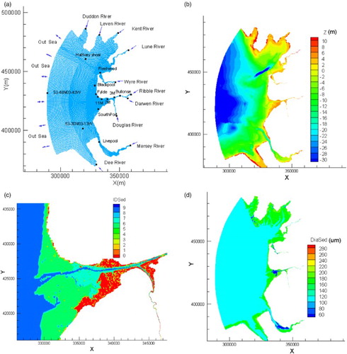
The open boundary conditions at the open seaward boundary included the tide levels obtained using a harmonic analysis from the MIKE21 software or the Irish Sea 2D hydrodynamic model based on EFDC-2D (Zhou et al. 2014). A constant salinity of 35 ppt, a temperature of 20.0°C, a SSC of 5 mg/l and a FC concentration of 100 cfu/100 ml were also assumed at the boundary. The corresponding parameter values included in the model at the upper riverine boundaries were: discharges, SSCs and FC levels (generally obtained from measured data), with additional values included for salinity of 0.2 ppt and a temperature of 18.0°C at all upper boundaries. The lateral point sources were obtained using measured data at present, but with numerical calculated results being obtained using the HSPF model and inforworks software, provided by Sheffield University, in the future. The time step was 0.3 s and with the variable data sources being interpolated at every time step in model simulations. The corresponding starting and end times are from 2 to 5 June 1999. The simulations took 1 day, with a single core processor with 3.4 GHz, for the SSC. One day was needed to obtain a stable state, and with 1.5 days being needed for the FIO, based on the concentration mainly being found to come from the rivers.

4.3 Model verification

4.3.1 Hydrodynamic predictions

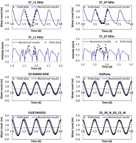
The predicted water levels generally agree well with the measured data at the selected comparison sites (Figure 1(a)) near the Ribble estuary, Morecambe Bay, Mersey Bay and the other regions (Figure 2). However, there are some errors in the calculated velocity, with the predicted peak values being smaller than the measured values. This discrepancy in the comparisons is thought to be due to discrepancies in the bathymetry, where linear interpolation has been used based on the cross-section sampling data. In addition, the few effective grid nodes along the narrow and deep main channel may cause some possible prediction errors, especially due to the difficulties in representing the narrow channel accurately in the 2D/3D model. These errors are being checked in further studies and it is expected that improved velocity predictions will be shortly obtained.

Figure 2 The verification of the water lever and velocity at the different monitoring sites.

4.3.2 Sediment predictions

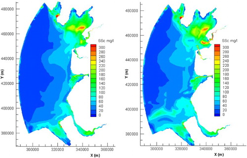
At present, there are no measured SSC data available at any of the monitoring sites during the same period, that is, from 2 to 5 June 1999. However, the predicted values are given according to discharge–sediment concentration relationships deduced from historical data. The predicted results show qualitatively that (Figure 3): (i) the high concentration regions ranging from 100 to 300 mg/l are located in the Morecambe, Ribble and Mersey estuaries, caused by erosion in the relatively large and shallow tidal deltas, under the action of the larger currents during spring tides, with the suspended sediment in the shallow tidal delta being transported up towards the river or down the estuary and along different directions before being deposited in these regions due to the reduced dynamic environment; (ii) the bathing region near the southern part of Blackpool, which may be impacted slightly by the sediment-laden current edge from the Morecambe Bay region during neap tides and with these sediment-laden flows bringing more faecal bacteria from the Wyre and Morecambe to the sandier bathing beaches near Blackpool. However, the sediment concentration distribution around the Fylde Coast is also strongly influenced by the suspended sediment flux from the river Ribble, including local erosion and deposition. The main component of sediment deposition around the river deltas of the Ribble and Wyre and the moderate hydrodynamic features, in terms of relatively low currents, may supply the ideal conditions for safe bathing in the Blackpool region. The model has been set-up to calculate the dynamic spatial distribution of the sediment concentration field for different inflow and tidal conditions. However, the predictions first need to be validated and verified using measured data, currently being acquired.

Figure 3 SSC distribution for spring (left) and neap (right) tides.

4.3.3 Faecal bacteria predictions

(1) Verification at measuring sites. Due to large variations in the predicted and measured FC concentrations, the results are plotted using a logarithmic scale. Figure 4(a) shows an example application of the original linked model to the Ribble estuary, where predicted and measured FC concentrations are compared at 3 Milepost. Comparisons were made for data acquired on 19 May 1999, which was carried out for a dry event and a spring tidal range. The statistical parameters used were the standard error (SE) and the averaged percentage (E), defined as follows:

Figure 4 Comparison of predicted and measured FC concentrations at 3 Milepost (upper) and 7 Milepost (lower) on 3 June 1999.

andwith SE = 477 cfu/100 ml and E = 27.6%. The predicted and measured FC concentrations at 7 Milepost for the survey on the 3 June 1999 were compared in Figure 4(b), with an SE = 35,000 cfu/100 ml, and E = 30.5%. As can be seen from this figure, both sets of data, that is, the measured and predicted values, agreed well. The predicted error may be increased from the narrow middle reach to the wide lower reaches of the estuary because of the coupling of multiple dynamic mechanisms and the additional uncertainty in the lower reaches of the river, the confluence of the Ribble and Douglas rivers, and the estuary region.

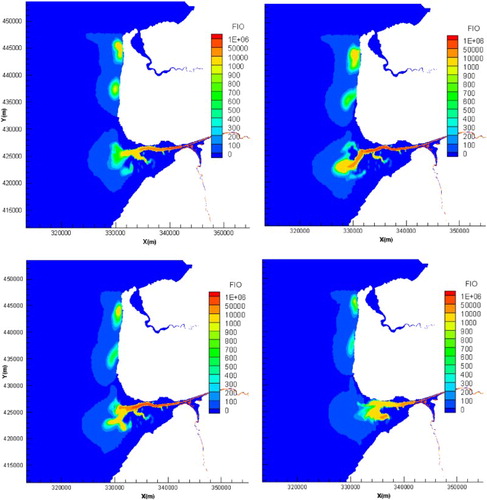
(2) Spatial distribution of FC concentrations. The spatial and temporal distributions of FC concentration distributions, as predicted using the model for four types of tides, are given in Figure 5. The results show that the high faecal concentration region (HFCR), with a concentration in the range 10,000 to 100,000 cfu/100 ml, is located mainly in the riverine region and the salt marshes in the Ribble delta. For the general case, the HFCR may move to and fro in the river basin based on the dynamic interactions between the river and estuary. The middle faecal concentration region (MFCR), which ranged from 1000 to 10,000 cfu/100 ml, tends to move more in a southwest direction along the Ribble main channel, under the action of the large inflow from the river and for neap tides, with the front of the MFCR arriving at Southport, to the south of the basin. In addition, the front of the MFCR frontier in the estuary may advect along the Fylde Coast to the North, especially under the action of southerly winds. The low faecal concentration region (LFCR) appears in the estuary by the advection, diffusion and dilution of the MFCR and HFCR in large water volume. The local point sources near Blackpool may have some local impact on the sand beach and may cause an MFCR for 1.0 and 2.0 km along the x- and y-directions, respectively. The LFCR may cover all of the sandy beaches along the Fylde Coast, including Blackpool. Hence, it is important to control the local polluted effluent discharges from the sewage outfalls near the bathing region, as well as the treated FC-laden flows from the river Ribble.

Figure 5 Distribution of FC concentration distributions for four tidal conditions (mid-ebb, low tide, mid-flood and high tide, units: cfu/100 ml).

5 Health risk analysis using the QMRA method

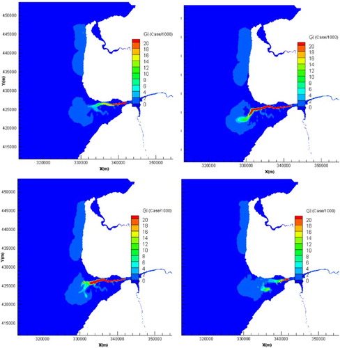
Based on the calculated FIO results (Figure 5), the spatial and temporal distributions of risk of acquiring GI cases per 1000 swimmers has been predicted using Eqs. (23a–24) with a middle ingestion rate of 35 ml/h. The results are shown in Figure 6 for different tidal conditions. According to the US EPA standards, the acceptable water health risk is 19 GI cases per 1000 persons, hence the FC concentration level is acceptable for the bathing water compliance according to the UK criteria at the bathing water beaches along the Fylde Coast, around Blackpool, and in the vicinity of Southport, from 2 to 5 June, 1999. However, for the revised EU Bathing Waters Directive (2006/7/EC) ((CEU) C.o.t.E.U., 2006), for coastal waters in the UK, the maximum value for intestinal enterococci and Escherichia Coli concentrations is 185 and 500 cfu/100 ml, respectively, for bathing water compliance. However, based on the old standards in 1976 ((CEC) C.o.t.E.C, 1976), the related maximum value is 2000 cfu/100 ml for the minimum faecal bacteria compliance. The predicted E. Coli concentration from the outfall near Blackpool may be as high as 700 cfu/100 ml, and the results show some small regions from the outfall where the plume is non-compliant with the new mandatory values which will need to be met in 2015 in the UK. However, the model predictions meet the requirement of the current standards in the UK using the value in 1976. The different interpretation of the results shows that the new water quality standard for bathing water compliance in the UK is stricter than the standards in the USA and current standards across the EU. The results indicate that the effluent would need to be treated further for compliance with the new bathing water quality standard in the UK.

Figure 6 Health risk results using the QMRA method for four tides (mid-ebb, low tide, mid-flood and high tide).

6 Further work currently planned

In continuing with this research project a number of steps of further research are planned, including the following: (i) quantitative prediction and analysis of the results for faecal process representation using different coupling methods between the sediment and water column interactions for the 2D and 3D models; (ii) a sensitivity analysis of the key parameters, especially T ₉₀ for different salinity, sediment and radiation conditions from the rivers to the estuary; (iii) local faecal organism levels from point sources in the middle and lower reaches of the basin may have increased contributions on the FIO flux into estuary due to urbanization, increased population densities and higher economic levels;. (iv) improved representation of the interface between the river and estuary, where there are dynamic and complex 3D structures and complex salinity and sediment concentration distributions for different river inflow discharges, tidal currents and wind-induced wave conditions; and (v) improvements in the implementation of the QMRA method, including a random frequency function and more uncertainty analysis in the ingestion dose and dose–response relationship for different age groups.

7 Conclusions

An integrated numerical model has been set up and refined to predict the fate and transport of faecal organisms from riverine to receiving coastal waters, using the EFDC-2D/3D and the FASTER-1D models. The key refinements to the existing codes include further developments and modifications in the coupling faecal bacteria interactions between the water column and suspended sediments, health risk analysis using the QMRA method and model linkages in which theoretical formulae are used relating the coupling between sediment transport and faecal bacteria adsorption/desorption processes. The model has been applied to the Ribble river and estuary, with predicted results being compared with measured data taken across the domain from 2 to 5 June 1999. The comparisons between the predicted and measured data generally agree well. The predicted spatial and temporal FIO concentration distributions, obtained from the integrated numerical model, give support to the integrated assessment of environmental exposure, health impacts and risk perceptions of faecal organisms in the coastal waters. In comparing these concentration distribution predictions with the water quality standards for bathing water compliance for the US EPA and the EU WFD for the UK, the dynamic spatial distribution of the peak concentration region is not always fully compliant with the mandatory and tighter microbial standards of the WFD. Finally, some further key challenges are presented in the paper and this work is currently ongoing.

Acknowledgements

The authors are grateful to the Environment Agency North West for their provision of data and to all colleagues from the universities of Aberystwyth and Sheffield working on the NERC C2C project.

Additional information

Funding

The research reported herein is funded by the Natural Environment Research Council, the Medical Research Council, the Department for Environment, Food and Rural Affairs and the Economic and Social Research Council [GR NE/I008306/1] UK. The third author is funded through a Case Studentship, funded jointly by CH2M HILL and the Natural Environment Research Council.

References

- Ashbolt, N.J., et al., 2010. Predicting pathogen risks to aid beach management: the real value of quantitative microbial risk assessment (QMRA). Water Research, 44 (16), 4692–4703. doi: 10.1016/j.watres.2010.06.048
- Bai, S. and Lung, W.-S., 2005. Modeling sediment impact on the transport of fecal bacteria. Water Research, 39 (20), 5232–5240. doi: 10.1016/j.watres.2005.10.013
- Benham, B.L., et al., 2006. Modeling bacteria fate and transport in watersheds to support TMDLs. Transactions of the ASABE, 49 (4), 987–1002. doi: 10.13031/2013.21739
- de Brauwere, A., et al., 2011. Modelling Escherichia coli concentrations in the tidal Scheldt River and estuary. Water Research, 45 (9), 2724–2738. doi: 10.1016/j.watres.2011.02.003
- de Brauwere, A., et al., 2014. Integrated modelling of faecal contamination in a densely populated river–sea continuum (Scheldt River and Estuary). Science of the Total Environment, 468–469, 31–45. doi:10.1016/j.scitotenv.2013.08.019
- Breuer, M., et al., 2012. Fluid–structure interaction using a partitioned semi-implicit predictor–corrector coupling scheme for the application of large-eddy simulation. Journal of Fluids and Structures, 29, 107–130. doi:10.1016/j.jfluidstructs.2011.09.003
- (CEC), C.o.t.E.C., 1976. Council Directive 76/160/EEC concerning the quality of bathing water. Official Journal of the European Communities, L31, 1–7. Available from: http://europa.eu/legislation_summaries/consumers/consumer_safety/l28007_en.htm [Accessed 2 July 2013].
- (CEU), C.o.t.E.U., 2006. Directive 2006/7/EC of the European Parliament and of the Council of 15 February 2006 concerning the management of bathing water quality and repealing Directive 76/160/EE. Official Journal of the European Union, L64, 37–51.
- Chapra, S., 1997. Surface water quality modeling, Series in Water Resources and Environmental Engineering. New York: Mc-Graw-Hill.
- Chen, N. and Hong, H., 2012. Integrated management of nutrients from the watershed to coast in the subtropical region. Current Opinion in Environmental Sustainability, 4 (2), 233–242. doi: 10.1016/j.cosust.2012.03.007
- Cho, K.H., et al., 2012. The modified SWAT model for predicting fecal coliforms in the Wachusett Reservoir Watershed, USA. Water Research, 46 (15), 4750–4760. doi: 10.1016/j.watres.2012.05.057
- Connolly, J.P., Blumberg, A.F., and Quadrini, J.D., 1999. Modeling fate of pathogenic organisms in coastal waters of Oahu, Hawaii. Journal of Environmental Engineering, 125 (5), 398–406. doi: 10.1061/(ASCE)0733-9372(1999)125:5(398)
- Eric Jones, J. and Davies, A.M., 2010. Application of a finite element model to the computation of tides in the Mersey Estuary and Eastern Irish Sea. Continental Shelf Research, 30 (5), 491–514. doi: 10.1016/j.csr.2010.01.003
- Field, K.G. and Samadpour, M., 2007. Fecal source tracking, the indicator paradigm, and managing water quality. Water Research, 41 (16), 3517–3538. doi: 10.1016/j.watres.2007.06.056
- Gao, G., Falconer, R.A., and Lin, B., 2011. Numerical modelling of sediment–bacteria interaction processes in surface waters. Water Research, 45 (5), 1951–1960. doi: 10.1016/j.watres.2010.12.030
- Gao, G., Falconer, R.A., and Lin, B., 2013. Modelling importance of sediment effects on fate and transport of enterococci in the Severn Estuary, UK. Marine Pollution Bulletin, 67 (1–2), 45–54. doi: 10.1016/j.marpolbul.2012.12.002
- Ghimire, B. and Deng, Z., 2013. Hydrograph-based approach to modeling bacterial fate and transport in rivers. Water Research, 47 (3), 1329–1343. doi: 10.1016/j.watres.2012.11.051
- Griffith, J.F., et al., 2009. Evaluation of rapid methods and novel indicators for assessing microbiological beach water quality. Water Research, 43 (19), 4900–4907. doi: 10.1016/j.watres.2009.09.017
- Gunduz, O. and Aral, M.M., 2005. River networks and groundwater flow: a simultaneous solution of a coupled system. Journal of Hydrology, 301 (1–4), 216–234. doi: 10.1016/j.jhydrol.2004.06.034
- Haas, C.N., Rose, J.B., and Gerba, C.P., 1999. Quantitative microbial risk assessment. New York: John Wiley & Sons.
- Haas, C.N., et al., 2000. Development of a dose-response relationship for Escherichia coli O157:H7. International Journal of Food Microbiology 56 (2–3), 153–159. doi: 10.1016/S0168-1605(99)00197-X
- Hamrick, J.M., 1992. A three-dimensional environmental fluid dynamics computer code: theoretical and computational aspects. Special Report 317. Gloucester Point, VA: Virginia Institute of Marine Science, College of William and Mary.
- Helmig, R., et al., 2013. Model coupling for multiphase flow in porous media. Advance in Water Resource, 51, 52–66. doi:10.1016/j.advwatres.2012.07.003
- Henley, J., 2013. England's polluted beaches: stop this tide of filth. Available from: http://www.theguardian.com/environment/2013/jul/07/england-polluted-beaches-tide-of-filth [Accessed 7 July 2013].
- Huang, G., et al., 2013. Distributed numerical hydrological and hydrodynamic modelling for large river catchment. In: Wang Zhaoyin, Joseph Hun-wei Lee, Gao Jizhang, and Cao Shuyou, eds. Proceed ings of the 35th IAHR World Congress, August 2013, Chengdu, China. Beijing: Tsinghua University Press, 1–12.
- Kashefipour, S.M., et al., 2002. Hydro-environmental modelling for bathing water compliance of an estuarine basin. Water Research, 36 (7), 1854–1868. doi: 10.1016/S0043-1354(01)00396-7
- Kashefipour, S.M., Lin, B., and Falconer, R.A., 2006. Modelling the fate of faecal indicators in a coastal basin. Water Research, 40 (7), 1413–1425. doi: 10.1016/j.watres.2005.12.046
- Kay, D., et al., 2005. Predicting faecal indicator fluxes using digital land use data in the UK's sentinel Water Framework Directive catchment: the Ribble study. Water Research, 39 (16), 3967–3981. doi: 10.1016/j.watres.2005.07.006
- Lai, X., et al., 2013. Large-scale hydrodynamic modeling of the middle Yangtze River Basin with complex river–lake interactions. Journal of Hydrology, 492, 228–243. doi:10.1016/j.jhydrol.2013.03.049
- Lane, A., 2004. Bathymetric evolution of the Mersey Estuary, UK, 1906–1997: causes and effects. Estuarine, Coastal and Shelf Science, 59 (2), 249–263. doi: 10.1016/j.ecss.2003.09.003
- Luo, J., et al., 2013. Numerical modelling of hydrodynamics and sand transport in the tide-dominated coastal-to-estuarine region. Marine Geology, 342, 14–27. doi:10.1016/j.margeo.2013.06.004
- Miller, G.C. and Zepp, R.G., 1979. Effects of suspended sediments on photolysis rates of dissolved pollutants. Water Research, 13 (5), 453–459. doi: 10.1016/0043-1354(79)90038-1
- Ouattara, N.K., et al., 2013. Modelling faecal contamination in the Scheldt drainage network. Journal of Marine Systems, 128 (2013), 77–88. doi:10.1016/j.jmarsys.2012.05.004
- Park, I.K., et al., 2013. An implicit code coupling of 1-D system code and 3-D in-house CFD code for multi-scaled simulations of nuclear reactor transients. Annals of Nuclear Energy, 59, 80–91. doi:10.1016/j.anucene.2013.03.048
- Pye, K., et al., 2010. Cell 11 regional monitoring strategy results of sediment particle size analysis. Report, 1. Kenneth Pye Associates Ltd., External Investigation Report EX1219, October 2010.
- Saul, A.J., et al., 2011. C2C CLOUD TO COAST: Integrated assessment of environmental exposure, health impacts and risk perceptions of faecal organisms in coastal waters, project report. Available from: http://www.shef.ac.uk/c2c [Accessed 2 October 2013].
- Shrestha, N.K., et al., 2013. OpenMI-based integrated sediment transport modelling of the river Zenne, Belgium. Environmental Modelling & Software, 47, 193–206. doi:10.1016/j.envsoft.2013.05.004
- Soller, J.A., et al., 2010. Estimated human health risks from exposure to recreational waters impacted by human and non-human sources of faecal contamination. Water Research, 44 (16), 4674–4691. doi: 10.1016/j.watres.2010.06.049
- Stumpf, C.H., et al., 2010. Loading of fecal indicator bacteria in North Carolina tidal creek headwaters: hydrographic patterns and terrestrial runoff relationships. Water Research, 44 (16), 4704–4715. doi: 10.1016/j.watres.2010.07.004
- Tetzlaff, D., Capell, R., and Soulsby, C., 2012. Land use and hydroclimatic influences on Faecal Indicator Organisms in two large Scottish catchments: Towards land use-based models as screening tools. Science of the Total Environment, 434, 110–122. doi:10.1016/j.scitotenv.2011.11.090
- Thomann, R.V. and Mueller, J.A., 1987. Principles of surface water quality modeling and control. New York, NY: Harper & Row Publishers.
- Tseng, L.Y. and Jiang, S.C., 2012. Comparison of recreational health risks associated with surfing and swimming in dry weather and post-storm conditions at Southern California beaches using quantitative microbial risk assessment (QMRA). Marine Pollution Bulletin, 64 (5), 912–918. doi: 10.1016/j.marpolbul.2012.03.009
- Wilkinson, J., et al., 1995. Modelling faecal coliform dynamics in streams and rivers. Water Research, 29 (3), 847–855. doi: 10.1016/0043-1354(94)00211-O
- Yang, L., et al., 2002. Integration of a 1-D river model with object-oriented methodology. Environmental Modelling & Software, 17 (8), 693–701. doi: 10.1016/S1364-8152(02)00029-4
- Zhang, H., et al., 2012. An integrated multi-level watershed-reservoir modeling system for examining hydrological and biogeochemical processes in small prairie watersheds. Water Research, 46 (4), 1207–1224. doi: 10.1016/j.watres.2011.12.021
- Zhou, J., Pan, S., and Falconer, R.A., 2014. Effects of open boundary location on the far-field hydrodynamics of a Severn Barrage. Ocean Modelling, 73, 19–29. doi:10.1016/j.ocemod.2013.10.006