Measurement of sewer sediments with acoustic technology: from laboratory to field experiments

Abstract

Monitoring sewer sediments is necessary to better understand sedimentation and erosion processes. Sonar is one of the available techniques to proceed to sewer sediment measurements. Extraction of numerical data, implementation of a new algorithm to identify the water-sediment interface, laboratory and field experiments have been done to evaluate the device, to quantify uncertainties and to test the sonar under various conditions. Results demonstrate that: 1) uncertainties in repeatability are less than 4%, 2) the sonar delivers accurate results under various conditions (small to large sewers and grit chambers), and 3) in situ measurements are affected by uncertainties, mainly due to the fact that the sensor is not in a fixed position but is floating on the free surface in the sewer. This device is useful and accurate for semi-automatic measurement but further research and improvements should be done to better know the position of the device in the section.

Keywords:

• Monitoring
• deposits
• ultrasonic measurement
• sonar
• uncertainties

Introduction

Sediments in sewers are the source of various problems and disturbances like hydraulic section reductions and premature overflows, odours and corrosion problems, and release of pollutants during peak flows and storm events (Ashley et al. 2004). It is thus necessary to cleanse sewers where they are not self-cleansing and where sediments may accumulate. Municipalities and operators spend a lot of financial and human resources to accomplish this task. In order to save resources and improve sewer operation and maintenance, a better understanding of sediments accumulation, erosion and transfer is necessary (Laplace 1991, Verbanck 1992, Bertrand-Krajewski et al. 2006). Measurements of sewer sediments allows the achievement of three goals: 1) to develop scientific knowledge on sediments and to improve sediment transport models, 2) to optimize the allocation of resources in cleansing sewers by means of decision models based on sedimentation rates and to later check the efficiency of cleansing and 3) to assess optimal positions of flushing gates for sediment scouring (e.g. Campisano et al. 2004, Bertrand-Krajewski et al. 2006, Creaco and Bertrand-Krajewski 2009). Few techniques are available for in situ sewer deposit measurements (e.g. Laplace et al. 1988, Lorenzen et al. 1992, Gourmelen et al. 2010, Velasco et al. 2014), including sonar measurements (e.g. Wotherspoon et al. 1991, Ristenpart 1995, Schellart 2007, Carnacina and Larrarte 2014, Hemmerle et al. 2014). This paper presents the results of the tests of a rotating sonar device to measure sediment profiles, based on antecedent experiments (Bertrand-Krajewski and Gibello 2008).

Preliminary tests and measurements under controlled laboratory conditions at INSA Lyon and in various sewer sections in the Barcelona sewer system (Pouzol 2011) demonstrated that sonar is able to deliver data suitable for sewer deposit measurements and with an accuracy compatible with the three above goals. Further research has then been done to: 1) implement a new algorithm to better locate the water-sediment interface, 2) evaluate the response of the probe to various types of sediment (sand, gravel, stones, sludge), 3) quantify the repeatability and the uncertainties of measurements and 4) evaluate influential factors on the measurement quality. A last series of field experiments has been performed in various sewers in Lyon, France to evaluate and demonstrate the potential operational application of sonar.

Materials, sites and methods

Materials

The Marine Electronics Model 1512 pipe profiling sonar device is designed to scan filled pipes. The probe emits acoustic waves (2 MHz) and records the strength and the time of the echoes. The device includes three sensors: a transducer driven by a motor (i.e. the sonar itself) and pitch and roll sensors. The device is connected to a cable providing electrical power and information exchange with a USB control box. A laptop is required to run the ME 1512 system software.

In order to obtain a cross-section sewer sediments profile, four steps are necessary:

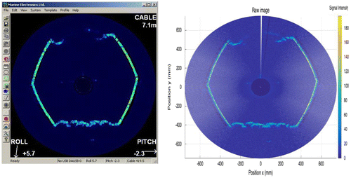
(1)	Scanning. The cross-section profile is scanned by internal rotation of the transducer. 400 sectors (angle of 0.9°) are measured to cover a full 360° rotation. Each sector includes 250 points equally distributed along the ultrasound beam ranging from 125 to 6000 mm (i.e. the distance between two points then varies from 0.5 mm to 24 mm). The pulse duration could be set from 4 to 20 μs. The sonar also measures roll and pitch angles: recorded images are corrected for the roll but not for the pitch (Marine Electronics 2012).
(2)	Displaying. Raw data images are displayed using a 256 colour scale, accounting for the roll/pitch position of the sonar (Figure 1, left). The user can process the raw data before the next step with four different parameters: threshold (filters out data below a given intensity), maximum (lowers the maximum intensity, therefore assigns the same value to high intensities), colour step (decreases the number of colours used to display the raw data) and blanking (relevant for the next step).
(3)	Profiling. Three algorithms are provided by the manufacturer (Marine Electronics 2012), named respectively the maximum, the ¾ maximum and the area algorithms, in order to identify, among the 250 points of each sector, the point corresponding to the water-sediment interface: a) the maximum: for each sector, the algorithm searches the closest point P1 from the sonar with the maximum intensity; b) the ¾ maximum: the algorithm searches the point P1 like the maximum algorithm and then selects the first point located between P1 and the sonar which presents a signal intensity equal to ¾ of the maximum intensity; c) the area: this algorithm selects the peak with the maximum total energy (a peak begins when intensity goes above a threshold and finishes when it returns below it).
(4)	Recording. Processed data can be recorded as .img files. Three types are available (A, B and C), with increasing levels of detail. Type C has been chosen for this study.

One to two seconds are necessary to go through all steps and obtain a cross-section sediment profile.

Figure 1. Screenshot of the ME software (left) and data extracted from the same raw measurement with the developed Matlab® code (right).

In the laboratory, the following materials have been tested as sediments: sand (Hostun sand, maximum grain size = 500 μm), gravels (diameter 6–10 mm), stones (mean diameter 20–30 mm), low concentration sludge (5–6% in mass) and high concentration sludge (30% in mass). The sludge was sampled from one of the Greater Lyon wastewater treatment plants to investigate loose water-sediment interface and to qualitatively observe how the sensor signal may differ in the presence of such material compared to sand and gravel.

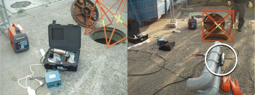
For field experiments, the “El Torpedo” prototype (adapted from Bertrand-Krajewski and Gibello 2008) initially built for the tests in Barcelona (Pouzol 2011) was reused in Lyon (Figure 2): the sonar has been fixed below the catamaran (built with two PVC downpipes) and the parallelism between sonar and catamaran main axes has been manually checked. For safety reasons, it is forbidden to introduce high voltage equipment into the Greater Lyon sewer system. This is why the transmitter and the generator remained outside the sewer (Figure 2, left), which restricted the length of the sewer reaches to be explored (due to the length of the cable between the transmitter and the sonar and the depth of the sewer to inspect). Along the measurable reach, the “El Torpedo” has been manually positioned in the flow: the stability of the catamaran and the accuracy of the position have been ensured by means of an aluminium bar, placed on both sides at pre-marked locations (1 m between each), to where the catamaran was pushed by the flow in the pipe. Thanks to this construction, the catamaran and the sonar were kept parallel to the lateral walls of the sewer and horizontal angles between the central axis sewer line and the central axis of the sonar were neglected.

Figure 2. Material used for field experiments in Lyon. Left: sonar equipment; right: the floating El Torpedo with the attached sonar probe (in the middle of the white circle).

In order to correct potential positional mistakes, a graphical tool has been implemented in the Matlab® code, based on superimposition of the theoretical and the measured profiles (pipe and sediments): singularities in pipe (such as sidewalk edges, angles) were helpful for this correction. If the singularity was above the free surface, the distance between the free surface (i.e. the sonar at a known depth below the surface) and this remarkable point has been measured with a ruler for each cross-section.

Sites

Laboratory facility

A series of tests was carried out in a T210 egg-shape concrete sewer pipe (height = 2.10 m) as this section is typical of the man-entry sections of the Greater Lyon sewer system. A 2 m long T210 pipe was installed at INSA Lyon laboratory. Its extremities were partly closed with metal plates and the sonar was installed inside the pipe along vertical bars allowing setting its position at different depths above the pipe invert. The pipe can be filled with potable water or wastewater at different depths, and various types of sediments (stones, gravels, sand, sludge) can be placed on the pipe invert.

Field experiments in Greater Lyon

Several sites (grit chambers, double side walk trunk sewers, etc.) have been investigated, each one representing one of the typical cases in Lyon where an improved technique for sediment monitoring is especially expected. All sites are located in large densely urbanised catchments in the city centre of Lyon equipped with combined sewer systems:

•	The first one is a 360 m3 grit chamber designed to trap grit and coarse sand in a large sewer upstream of a wastewater treatment plant. The dimensions of the grit chamber are 30 m long, 3 m wide and 4 m deep. 28 sediment profiles with an equidistance of 1 m have been measured with the sonar along the chamber.
•	The Quai des Etroits sewer is an asymmetrical trunk sewer with sidewalks and a 1.2 m wide dry weather channel. 24 sediment profiles with an equidistance of 1 m have been measured in the dry weather channel along a 22 m long reach.
•	The Guillotière sewer is a 1.4 m large pipe without a dry weather channel and with a rather flat invert. 14 sediment profiles with an equidistance of 1 m have been measured along a 12 m long reach.
•	The Maison de l’eau sewer is a 4 m wide trunk sewer with sidewalks and a dry weather channel prone to sedimentation. 14 sediment profiles with an equidistance of 1 m have been measured along a 12 m long reach.

Methods

Access to and conversion of raw data

In the standard mode of operation, the ME 1512 sonar delivers only images with a colour scale from 0 to 255 for signal intensity (Figure 1, left) and interface profiles represented as superimposed white lines after the interface detection algorithm is applied. There is no access to raw data files. In order to test a new algorithm and facilitate data processing, access to raw data is a pre-requisite. For this research, the manufacturer agreed 1) to explain how to access the raw image data and 2) to describe how raw image data are coded in the software tool. The image files (format .img) raw data are coded in hexadecimal notation and need to be translated into numerical values for further calculations. A Matlab® code has been written to extract numerical values from the .img files (Figure 1, right). The comparison between both pictures highlights that the graphical representations are the same and allows a validation of the Matlab® code. The advantage of the self-programmed method is the access to numerical values of the echo strength.

Implementation of a new algorithm

The maximum and ¾ maximum algorithms provided by the manufacturer (details of equations are not available to the user) are usually applied to detect the water-sediment interface. From the preliminary laboratory tests, a new algorithm based on the maximum gradient of the intensities along each sector instead of the absolute values of intensities was suggested in Pouzol (2011) as a possible solution to improve the accuracy of the position of the water-sediment interface.

The proposed maximum gradient algorithm includes three main steps: 1) for each sector, the gradient of the intensity signal is calculated, using the diff function in Matlab®, as a vector with 249 gradient values, 2) the position P_k of the maximum gradient in the sector k is determined (Equation (1)) and 3) the water-sediment interface is set to this position and its distance from the sonar is equal to the distance of the position P_k :

(1)

where P_k is the position index of the water-sediment interface along the signal vector corresponding to the sector k, R is the signal intensity for point j (intensity value between 0 and 255). Only sectors under the free surface are considered in the calculation of P_k. It is important to note that, as there are always 250 points in each sector with an equidistance ranging from 0.5 mm to 24 mm, the position of the maximum gradient is known accordingly with an uncertainty ranging from ±0.5 mm to ±24 mm: the longer the distance between the sonar and the sewer walls (from 125 mm to 6000 mm), the higher the uncertainty in the position of the water-sediment interface.

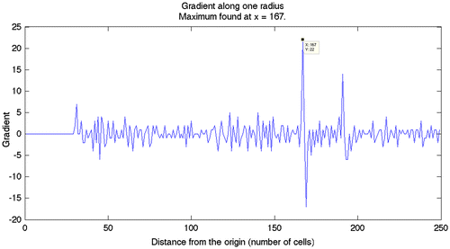
An example of signal gradient along a sector is given in Figure 3. The maximum gradient is observed in cell nr 167: its value is equal to 22. The algorithm is applied to all sectors: 400 positions of the maximum gradient measured from the central axis of the sonar are determined. As sector angles and the pitch are known, it is then easy to display the 400 positions of the maximum gradient in Cartesian coordinates and to correct the data.

Figure 3. Example of signal intensity gradient along a scanned sector (distance from the origin x = 0 corresponds to the central axis of the sonar probe).

Such an algorithm (based on gradient) might be sensitive to noise and artefacts. During all laboratory and in situ experiments, the noise/signal ratios have been quite low: any need of image pre-treatment popped up during the study. Identification and correction of artefacts are described hereafter.

Validation of data

For various reasons, artefacts or offsets in the position of the interface can be observed. Before calculation of the sediment area for each cross-section, manual corrections have to be done:

(1)

Removal of outliers. Sometimes a few points along the identified water-sediment interface are not realistically positioned and need to be removed. The robust identification has been performed with a common identification of the interface by the various algorithms.

(2)

Accurate identification of the boundary between sediment and pipe walls. The accuracy can be improved by an adequate selection of the measuring range (to reach the largest half-distance of the cross-section): this allows the optimization of the axial resolution (size of the cells) along the radius. For a pipe of 400 mm diameter, the range can be selected from 125 mm (minimum distance, with cell size of 0.5 mm) to 400 mm (maximum possible distance, with cell sizes of 1.6 mm).

Calculation of sediment areas and volumes

The cross-section profile of the sewer pipe without sediments is needed for these calculations. It can be either measured (best solution) or extracted from a GIS or any other database. By translation, the validated measured sediment profile is superimposed to the sewer pipe profile. The cross-section area (m²) of sediments is then calculated by integration of the difference between the pipe without sediments and the validated sediment profile, from the left to the right side of the pipe. When successive cross-sections are measured, it is then possible to estimate the sediment volume (m³) by interpolation between cross-sections and integration along the explored sewer reach. The sediment volume is more accurate if the distance between successive cross-sections is short (maximum a few metres). A preliminary quick exploration may help to determine the space step according to the variability of the sediment depths and areas along the sewer reach.

Laboratory experiments

The various types of sediments (sand, gravels, stones, sludge) have been placed on PVC plates to simulate sediment widths equal to 20, 30, 40, 50 and 80 cm. The sonar was located at a constant height in the T210 sewer cross-section, the distances between the sonar and the PVC plate being respectively equal to 53, 50, 46, 41 and 13 cm. Three pulse durations have been investigated: 4, 12 and 20 μs. Sediment profiles have been determined by means of four algorithms: maximum (named M), ¾ maximum (named ¾), maximum gradient (named G) and the area 1 (named A) which elaborates the profile according to points which have been included in the three previous profiles by at least two of the three algorithms. For each case, five profiles have been measured repeatedly.

Results and discussions

Laboratory experiments

Maximum gradient algorithm

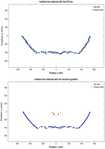
The results obtained with M and ¾ algorithms are similar (Figure 4, top shows results with M algorithm). In the centre of the pipe, sandy sediments are present and sediment profiles are clearly determined. However, the interface is rather fuzzy for both algorithms, especially along the sewer walls. The ¾ interface line is slightly less fuzzy than with the M algorithm. The interface line obtained with the G algorithm is smoother than with the two previous ones, especially along the sewer walls (Figure 4, bottom), which significantly improves the accuracy of the superimposition of the sewer profile with the measured sediment profile. Some artefacts can be seen with the G algorithm but can be easily removed by looking for the points common with both M and G algorithms.

Figure 4. Water-sediment interface by the ¾ (top) and G (bottom) algorithms (Position x = 0 corresponds to the centre of the sewer pipe, position y = 0 corresponds to the central axis of the sonar probe).

Repeatability and uncertainty

Table 1 gives the coefficient of variation CV (in %) of repeated measurements of sediment areas for sand, gravel and stones for the 20 cm plate width. Table 2 gives the coefficient of variation CV (in %) of repeated measurements of sediment areas for 5% and 30% concentration sludge for the 50 cm plate width. CV can be interpreted as an order of magnitude of the repeatability relative standard uncertainty. Other results for other plate widths are similar and are not reported here.

Table 1. Relative standard uncertainty (in %) in sediment areas for sand, gravels and stones for a PVC plate width of 20 cm.

Material		Sand				Gravels				Stones
Algorithm		M	¾	G	A	M	¾	G	A	M	¾	G	A
Pulse duration (μs)	4	0.28	0.51	0.31	0.53	0.18	0.28	0.40	0.59	0.51	0.90	0.68	1.31
	12	0.31	0.91	0.08	0.36	0.18	0.53	0.35	0.97	0.27	1.91	0.31	1.15
	20	0.73	1.95	0.11	0.51	0.44	0.61	0.49	0.90	0.76	0.70	3.44	3.58

Table 2. Relative standard uncertainty (in %) in sediment areas for 5% and 30% concentration sludge for a PVC plate width of 50 cm.

Material		Sludge 5%				Sludge 30%
Algorithm		M	¾	G	A	M	¾	G	A
Pulse duration (μs)	4	0.14	0.13	0.10	0.08	0.20	0.53	0.33	0.45
	12	0.12	0.12	0.16	0.19	0.43	0.15	0.25	0.73
	20	0.12	0.21	0.65	0.39	0.08	0.14	0.44	0.87

Except for stones with the largest pulse duration and with algorithms G and A, CV values are lower than 2%, and globally 90% of CV values are lower than 1%. No algorithm performs better for repeatability than the other ones for all cases. This repeatability under stable laboratory conditions is excellent. For in situ experiments where coarse mineral sediments were the most predominant type of material, the main source of uncertainty is the determination of the position of the sonar in the cross-section and the stability of the sensor during the experiments. It is important to note that in the case of the 5% concentration sludge, the sediments are too liquid to be detected as an interface: the interface detected by the sonar is in reality the top of the PVC plate. Results are different with the 30% concentration sludge (collected after dewatering process in a WWTP) disposed as large aggregates on the PVC plate: this type of sludge is dense enough to be detected with a well-defined water-sediment interface. Even if research objectives and experimental conditions were different, these observations are consistent with the results reported by Carnicina and Larrarte (2014) who investigated the response of the same sonar for sewer sediments of types A (compact coarse mineral material) and C (loose fine organic particles) according to the sediment classification proposed by Crabtree (1989): the type A sediment generates a signal with a different gradient profile (single gradient peak i.e. well defined interface) than type C sediment (multiple gradient peaks and less accurate determination of the interface).

Regarding the influence of the distance between the sonar and the sediment interface, the experiments for sand, gravels and stones with a pulse duration of 4 μs were used for data analysis. The hypothesis to be tested was that shorter distances lead to lower uncertainties, because shorter ranges can be applied (the cell sizes decrease) and there are more sectors to describe the same deposit. Experiments confirm that relative standard uncertainty decreases when the distance between sonar and sediment decreases. However, this conclusion is valid only if the entire sediment profile can be measured, which is the case only in narrow sections and for smooth profiles. In other cases, shadow effects may occur and only a part of the deposit can be measured.

Field experiments

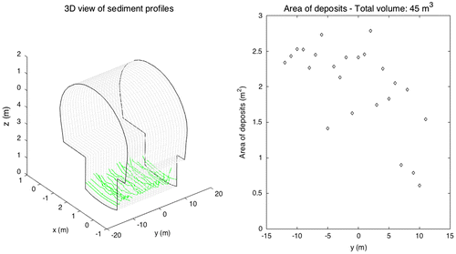
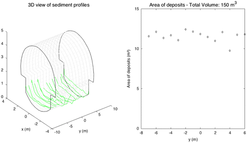
For each figure in this paragraph, the left part displays a 3D view of the measured cross-section sediment profiles, where black and grey lines indicate the sewer geometry and green lines represent the sediment profiles. The right part represents the sediment area (in m²) for each profile along the explored sewer reach.

Figure 5 shows the results for the Quai des Etroits grit chamber. Sediment profiles and filling rates vary enormously along the chamber, due to the hydrodynamics and sediment transport processes within the chamber. At the upstream extremity (x = 30 m from the reference point), there are very few sediments, due to a local strong recirculation zone which hinders settling. At the downstream extremity (x = 0 m), there are also less sediments, but as the recirculation zone is weaker, the filling rate is higher than at the upstream extremity. Sediments accumulate most for distances x from 5 to 20 m, with sediment depth above 2 to 2.5 m and sediment areas between 7.5 and 9 m². The 3D view also shows no lateral symmetry of the sediment profiles: it appears that sediment depths are higher along the right wall of the chamber, due to the hydrodynamic structures across the chamber. The total sediment volume in the chamber is estimated to be 188 m³ (50% filling).

Figure 5. 3D view of sediment profiles (left) and sediment area in m² (right) along the grit chamber at Quai des Etroits. The grit chamber was completely filled with water during the measurements.

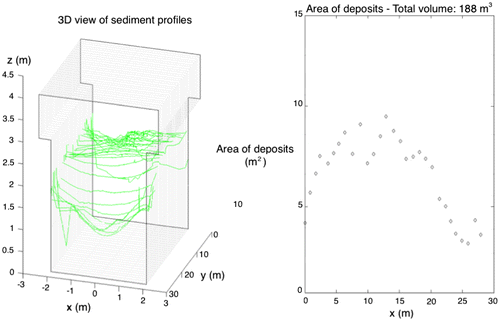
Figure 6 shows the results for the Quai des Etroits sewer. The total volume of sediment is 4.5 m³. The variability of the sediment areas along the reach is very significant, ranging from 0.06 to 0.27 m². The longitudinal sediment profile is very complex and the total volume of sediments could not be accurately estimated with traditional manual point measurements between manholes.

Figure 6. 3D view of sediment profiles (left) and sediment area in m² (right) along the Quai des Etroits sewer.

In the Guillotière sewer (Figure 7), the total volume of sediment is 4.56 m³, with rather homogeneous sediment profiles and areas. In the Maison de l’eau sewer (Figure 8), sediment areas range between 0.95 and 1.25 m² along the reach and the total volume of sediment is 15.1 m³.

Figure 7. 3D view of sediment profiles (left) and sediment area in m² (right) along the Guillotière sewer.

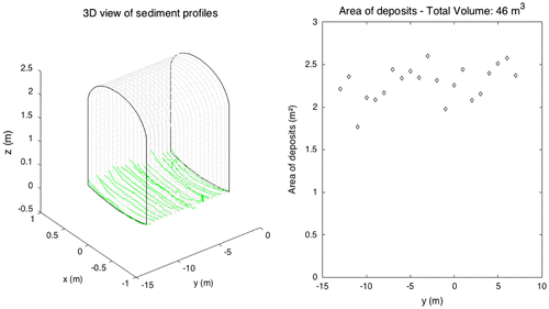
Figure 8. 3D view of sediment profiles (left) and sediment area in m² (right) along the Maison de l’eau sewer.

The experiments show that the sonar is suitable to measure sediment deposits in various sewer structures and allows a relatively accurate estimation of the sediment volumes, providing relevant data for cleansing planning. Repeated measurements at the same location over time will provide data about the net deposition rate (balance of erosion and sedimentation) and might be used for maintenance management (mid-term plan) and/or diagnostic of the current status of the pipe.

Conclusions and perspectives

A new gradient algorithm has been proposed and tested to better estimate water-sediment and sewer wall interfaces. The maximum gradient algorithm results in a better accuracy, especially for sewer wall detection. This improves the accuracy of the superimposition of the sewer pipe profile with the sediment profile. An additional step of data checking and validation has been added in a Matlab® code aiming to automatically calculate sediment areas and volumes.

Laboratory experiments shows that: 1) there is no measurable effect of the pulse duration in the range 4–20 μs under the conditions of the experiments, 2) repeatability, relative standard uncertainty in sediment areas under laboratory stable conditions is usually lower than 1% and always less than 4%, 3) if the sediment material is sufficiently dense and rough enough, its grain size has no measurable effect on uncertainties and 4) relative standard uncertainty in sediment areas decreases when the distance between sonar and sediments decreases.

Tests in real sewers have confirmed that the sonar is able to measure satisfactorily sediment profiles in various geometries. However the sonar cannot deliver good results in cases of very wide cross-sections with flat inverts and low water levels. The El Torpedo prototype used in the experiments presented in this paper is a basic piece of preliminary research equipment and is not specifically designed to perform routine sediment monitoring by practitioners. For routine operation, the sonar should be one part of a complete set of sonar monitoring equipment to be further developed.

Funding

The authors thank the FP7 PREPARED project (www.prepared-fp7.eu, EU contract nr 244232) for funding the work.

Acknowledgements

The authors thank the Greater Lyon and Clabsa for assistance and collaboration in field tests, and Alan Green from Marine Electronics Ltd for access to raw data of the sensor.

References

- Ashley, R.M., Bertrand-Krajewski, J.-L., Hvitved-Jacobsen, T. and Verbanck, M., 2004. Solids in Sewers. Scientific and Technical Report no. 14. London: IWA Publishing.
- Bertrand-Krajewski, J.-L., Bardin, J.-P. and Gibello, C., 2006. Long term monitoring of sewer sediment accumulation and flushing experiments in a man-entry sewer. Water Science and Technology, 54 (6–7), 109–117.
- Bertrand-Krajewski, J.-L. and Gibello, C., 2008. A new technique to measure cross-section and longitudinal sediment profiles in sewers. In: Proceedings of the 11th International Conference on Urban Drainage, Edinburgh, UK, 31 August–5 September 2008, 9.
- Campisano, A., Creaco, E. and Modica, C., 2004. Experimental and numerical analysis of the scouring effects of flushing waves on sediment deposits. Journal of Hydrology, 299, 324–344.
- Carnacina, I. and Larrarte, F., 2014. Coupling acoustic devices for monitoring combined sewer network sediment deposits. Water Science and Technology, 69 (8), 1653–1660.
- Crabtree, R.W., 1989. Sediments in sewers. Journal of the Institution of Water and Environmental Management, 3 (6), 569–578.
- Creaco, E. and Bertrand-Krajewski, J.-L., 2009. Numerical simulation of flushing effect on sewer sediments and comparison of four sediment transport formulas. Journal of Hydraulic Research, 47 (2), 195–202.
- Gourmelen, L., Cottineau, L.-M., & Larrarte, F., 2010. Développement d’un dispositif de mesure en continu de la hauteur de sédiments. Actes des Journées Génie Civil Génie Côtier, Les Sables d’Olonnes, France, 22-25 Juin 2010, 477–484 [ in French].
- Hemmerle, N., Randrianarimanana, J.-J., Joannis, C. and Larrarte, F., 2014. Hydraulics and deposit evolution in sewers. In: Proceedings of the 9th International Symposium on Ultrasonic Doppler Method for Fluid Mechanics and Fluid Engineering, Strasbourg, France, 27–29 August 2014, 9–12.
- Laplace D., 1991. Dynamique du dépôt en collecteur d'assainissement. Thesis (PhD). Institut National Polytechnique de Toulouse, France.
- Laplace, D., Dartus, D. and Bachoc, A., 1988. Développement d’un dispositif de mesure « en continu » de la hauteur de dépôt en collecteur d’assainissement. Toulouse, France: IMFT, rapport n° 398 IMFT/ESL [ in French].
- Lorenzen, A., Willms, M. and Dinkelacker, A., 1992. The Göttingen boat. Water Science and Technology, 25 (8), 57–62.
- Marine Electronics, 2012. Operators Manual Model 1512PC Pipe Profiling Sonar, 17 December 2012. Available from: http://www.marine-electronics.co.uk/Manuals/1512%20OM.pdf [Accessed 1 July 2015].
- Pouzol, T., 2011. Monitoring sediments in sewers with a rotating sonar. Thesis (MSc): INSA Lyon, France.
- Ristenpart, E., 1995. Feststoffe in der Mischwasserkanalisation, Vorkommen, Bewegung und Verschmutzungs-potential. Thesis (PhD). Hannover University, Germany, Schriftenreihe Stadtentwässerung und Gewässerschutz, Heft 11 [in German].
- Schellart, A.N.A., 2007. Analysis of uncertainty in the sewer sediment transport predictions used for sewer management purposes. Thesis (PhD). University of Sheffield, UK.
- Velasco, M., Suñer, D., Bertrand-Krajewski, J.-L., Aldea Borruel, X., and Pouget, L., 2014. Development of technical guidelines for the monitoring and modelling of sediments. Deliverable D3.2.4 of the FP7 European Project PREPARED, April 2014. Available from: http://www.prepared-fp7.eu/prepared-publications [Accessed 1 July 2015].
- Verbanck, M., 1992. Field investigation on sediment occurrence and behaviour in Brussels combined sewers. Water Science and Technology, 25 (8), 71–82.
- Wotherspoon, D.J.J., Ashley, R.M. and Woods, S.P., 1991. Imaging in sewer systems. In: J.W.S. Maxwell, ed. Applications of information technology in construction. London: Thomas Telford Ltd, 143–156.