Validation of 2D shock capturing flood models around a surcharging manhole

Abstract

This work offers a detailed validation of finite volume (FV) flood models in the case where horizontal floodplain flow is affected by sewer surcharge flow via a manhole. The FV numerical solution of the 2D shallow water equations is considered based on two approximate Riemann solvers, HLLC and Roe, on both quadrilateral structured and triangular unstructured mesh-types. The models are validated against a high resolution experimental data-set obtained using a physical model of a sewer system linked to a floodplain via a manhole. It was verified that the sensitivity of the models is inversely proportional to the surcharged flow/surface inflow ratio, and therefore requires more calibration from the user especially when concerned with localised modelling of sewer-to-floodplain flow. Our findings provide novel evidence that shock capturing FV-based flood models are applicable to simulate localised sewer-to-floodplain flow interaction.

Keywords:

• Floodplain flow
• sewer overflow
• dual drainage experiments
• approximate Riemann solvers
• shallow water equations
• quadrilateral vs triangular meshes

Introduction

During pluvial flood conditions, overland surface flow and surcharged sewer overflows may interact at exchange points such as manholes and gullies (Falconer et al. 2009). Such a localised phenomenon of urban flooding is complex and highly three dimensional (3D). Nonetheless, 3D modelling of these events system yields prohibitive runtime costs and is currently unforeseeable at street scale in the urban environment (Cea et al. 2010). Practically, it has become common to tackle modelling of sewer-to-floodplain flow interaction as a compound system consisting of 2D surface and 1D sewer-flow systems (Chen et al. 2015, Leandro et al. 2016, Lee et al. 2013, Martins et al. 2016, Seyoum et al. 2012).

The surface-flow is commonly termed the major system. It is often modelled using the depth-integrated Navier-Stokes Equations, termed shallow water equations (SWE), or one of the SWE simplifications in 1D or 2D, which can be numerically solved using a variety of approaches common in computational hydraulics (Kesserwani and Wang 2014, Neal et al. 2012, Martins et al. 2015, Leandro et al. 2014). Due to its inherent ability to incorporate flow transition, including shocks, the finite volume (FV) approach of Godunov has gained popularity in solving the fully dynamic SWE when modelling 2D floodplain flow. It has therefore become more frequently adopted in environmental modelling software tools and flood risk assessment applications (Néelz and Pender 2012). In particular, first-order models, based on Roe and/or HLLC families of Riemann solvers, are now widely used for real-world flood modelling.

A major complexity in modelling of urban flooding is the interaction of the major system and surcharging sewer flows via gullies and manholes. Excess flow or sewer choking (i.e. an abrupt transition from free surface to pressurized pipe, Hager (2010)) are often reasons for this surcharge. Zhao et al. (2004, 2006) performed an experimental study to investigate the phenomena at a pipe junction that frequently surcharged by studying two inlet configurations (angled at 90º and 25.8º) showing that three distinct flow regimes exist. Pipe pressurisation and overflowing from the manhole has the potential to induce a circular shock-wave into the surface flooding (Mahdizadeh et al. 2012). From a numerical modelling perspective, the surcharging discharge component is often calculated in the manholes and added to the surface-flow system via additional sink/source terms in the SWE, in order to model the hydrodynamic of sewer-to-floodplain flow. Though this approach assumes that the system is full, it represent a worst-case scenario for flood hazard and is worth an assessment as such. Hence, the reliability of this addition is yet to be assessed.

Fully-coupled approaches involve implicit coupling, of a 1D or 2D surface flow model, with a 1D unsteady pipe flow solver (Chen et al. 2015, Djordjević et al. 2005, Lee et al. 2013, Martins et al. 2016, Seyoum et al. 2012). In many of these works, sewer overflow is accounted for using only one computational cell, and for real-site applications (Martins et al. 2016). Alternatively, non-coupled shock-capturing FV models have also been adjusted to model sewer-to-floodplain flows. Partially coupled solutions Mahdizadeh et al. (2012) were tested under the assumption of full-pipe flow. Borsche and Klar (2014) presented a fully-integrated approach with sewer flow variability. To date, surcharged flow around the exchange area has not been fully characterised at both experimental and numerical levels (i.e. concerning 2D floodplain modelling in the vicinity of the manhole).

This paper presents a detailed verification of FV models against an original high-resolution experimental data-set using a physical model of a sewer system linked to a floodplain via a scaled manhole. Experiments are conducted under steady state discharge conditions to produce systematic increase in the sewer surcharge rate into a shallow flow over a floodplain. Two well-established FV numerical solvers to the 2D SWE are selected based on two approximate Riemann solvers, HLLC and Roe, and on different (non-uniform) mesh-types, i.e. quadrilateral structured and triangular unstructured, respectively. Comparing results from different meshes and schemes has been shown to be a valid methodology for benchmarking and validating models (see for example Neal et al. (2012) and Néelz and Pender (2012)). The FV models are adapted to the experimental domain and conditions. The FV models capacity to simulate hydraulic head at six sampling points and jump position around the surcharged manhole is assessed and discussed.

Methodology

Physical model

A physical model (Figure 1) at the University of Sheffield (Rubinato 2015) was used in comparing the results of numerical models. It is composed of a piped sewer system connected to a floodplain via a scaled manhole without a lid (manhole diameter = 240 [mm]) allowing free inflow and outflow from the manhole. Flows into the sewer and the floodplain can be controlled independently via automated in line valves such that a range of floodplain (surface) / pipe (sewer) flow exchange scenarios can be reproduced. The sewer system is horizontal, whereas the floodplain is inclined with a slope of 0.001 [m m⁻¹]. The main pipe of the sewer system (Figure 1) has a 75 [mm] inner diameter. The sewer system and manhole were constructed from acrylic.

Figure 1. 3D representation of the experimental facility, pressure transducer locations, mesh details and inflow details.

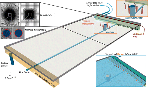
The floodplain has a length of l = 8.2 [m], a width of b = 4 [m] and side walls of height 0.1 [m]. Upstream inflow and downstream outflow tanks are the full width of the floodplain. Flow enters the inflow tank and spills over a weir into the floodplain. The upstream tank is filled with a baffle to ensure even inflow.

Calibrated electro-magnetic (MAG) flow meters were used to record discharge at the surface and sewer inlets (Q₃) and sewer outlet (Q₄) of the facility. The accuracy of the flow meters has been validated using volumetric discharge readings based on the laboratory measuring tank (error within 2.5% in all cases). GEMS series 5000 pressure transducers were installed to measure hydraulic heads at six locations around the manhole. The location of the transducers is presented in Figures 1, 2, and 4. Average transducer calibration deviation was ±0.109 [mm]. For each test conducted photos were taken 1.5 [m] vertically from the floodplain.

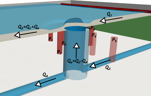
Figure 2. 3D representation of manhole/surface exchange location with surface inflow (Q₁), surface outflow (Q₂), sewer inflow (Q₃) and sewer outflow (Q₄) and depth measurement locations (P_x) around the manhole.

Experimental tests

Ten steady flow experiments were conducted. For each test, after flow stabilisation, flows and depths were recorded for 300 [s] (which was deemed sufficient to ensure convergence of measurements) and temporally averaged to provide mean values. For each test the surcharge rate (Q_e) and surface outflow (Q₂) are defined based on mass conservation principles (Equation (1(1) ) and (2(2) )).(1) (2)

Direct inflow to the surface inlet (Q₁) was kept approximately constant in all experimental cases (5.69 [l/s]) thus allowing an analysis based solely on the effect of the manhole surcharge. The sewer pipe inlet discharge (Q₃) was varied between tests in order to produce surcharge (Q_e) that constitutes a ratio of 0.37 to 0.91 of the surface inlet (Q₁).

Numerical models

In a conservative matrix form, the SWE including sewer source term reads:(3)

In Equation (1(1) ), (x, y) are the spatial Cartesian coordinates and t is the time. is the vector containing the flow variables, and and are the Cartesian components of the flux vectors. is the vector of source terms that, can be decomposed into (4) (5)

In Equations (4(4) ) and (5(5) ) g [m s⁻²] is the constant gravitational acceleration; h [m] is the water depth, hu and hv [m² s⁻¹] are the unit-width discharge expressed in terms of the velocity Cartesian components u and v [m s⁻¹]. and are, respectively, the topography and friction source terms involved in the momentum equations with C_f = gn² h^−1/3 (n is the Manning coefficient). denotes a sewer flux term involved in the continuity equation in terms of vertical velocity V_s, which represents a sewer surcharge into the floodplain; whereas u_bed and v_bed denote the local (i.e. non-depth averaged) horizontal velocities at the bed level (taken as zero for all simulations, i.e. u_bed = 0 and v_bed = 0).

HLLC approximate solver on structured quadrilateral mesh

The domain is discretised into computational quadrilateral cells. A computation cell is centred at (x_i, y_i) and has the dimension of dx_i × dy_i. A local piecewise-constant solution is sought over , and updated in time as:(6)

In Equation (6(6) ), the superscript n denotes the present time status and the time step evaluated under the Courant-Friedrichs-Lewy (CFL) criterion with a Courant number of 0.5 (where and represent the length of a cell). The time step is therefore controlled by . The interface fluxes across eastern, western, northern and southern faces of cell (i.e. , , and ) are obtained by the HLLC approximate Riemann solver (Toro et al. 1994). Bed, friction and sewer source terms are discretised in a local cell-centred manner (Wang et al. 2011).

The initial number of quadrilaterals has been chosen to be 41 × 20 to generate a baseline (coarse) mesh with a spatial resolution of around 0.2 [m] × 0.2 [m]. A mesh convergence analysis suggested the need to involve a (4×) finer mesh. This resulted in an adaptive mesh size with cells up to 0.0125 [m] × 0.0125 [m]. The final mesh has 11416 computational cells.

Roe approximate solver on unstructured triangular mesh

For the sake of comparison, the mesh was computed using the minimum and maximum edge lengths from the quadrilateral mesh and a similar growth rate (i.e., of 0.025). Cell edges near the manhole have a length of 0.0125 [m] with an increase in size up to 0.2 [m] near the external boundaries (Schöberl 1997). This results in a mesh with almost similar number of computational cells (i.e. 11186). The conservative discrete form of Equation (3(3) ) on a mesh element is:(7)

Where is a generic cell represented by its centre i, I_j are adjacent neighbours across the set of neighbouring points , A_i the computational area of , , and are the numerical fluxes evaluated based on the upwind Roe solver (Nikolos and Delis 2009). The bed elevation source term () is derived using an upwind scheme, respecting the extended C-property and therefore avoiding non-physical oscillations. Here, is evaluated using similar CFL to the HLLC provided that the cell dimensions are equal.

Boundary and initial conditions

Two different upstream boundary conditions were created for the solvers. The first is obtained by averaging all the inflows and outflows. The second is obtained considering the flow upstream (Q₁) skewed due to the lateral insertion of the flow in the upstream inflow tank (see Figure 1). Values for the skewed flow were calculated based on 2/3 weight of inflow inserted into the floodplain along the first 2 [m], after the lateral inlet, whilst the remaining 1/3 of the inflow would be distributed along the other 2 [m].

The surcharged sewer discharge Q_e is fed into the numerical model through V_s (i.e. Q_e divided by the manhole area) in the source term . Downstream, uniform flow and conservation of mass is enforced. This is judged appropriate because the floodplain is regular, the outlet is sufficiently far from the manhole and there is no restriction to the outlet flow. Depths are calculated using Equation (8(8) ) by enforcing the unitary outflows .(8)

Where n is the Manning’s roughness, taken as 0.011[s m−1/3], based on the average of the range of values given in Chow (1959) (0.008 to 0.01) and Smajstrla et al. (1985) (0.012 to 0.014) for the facility bed material (polypropylene), ∂_xz is the floodplain slope, b the width and h₂ the uniform depth at the outlet. The velocity is calculated through conservation of mass. These values were used as the initial condition for the models for faster convergence to the steady state solution. The unsteady flow models are run using the steady boundary conditions until convergence to a steady state is attained.

Analysis, results and discussions

Quantification of flow measurement error

To estimate the potential scale of the error introduced in Q_e and Q₂ due to flow oscillations, a statistical study is performed considering the observed averages and standard deviations for Q₁, Q₃ and Q₄. Using Equation (9(9) ), are estimated based on the 95% confidence intervals of Q₁, Q₃ and Q₄, considering the worst case scenario.(9)

with(10)

Standard deviations for Q₁ and Q₃ are 0.01 [l/s] and 0.05[l/s] for Q₄. Based on Equations (9(9) ) and (10(10) ) this results in a maximum difference in Q_e of approximately 5 [%] for the lowest flowrate. The average difference between the upper and lower limit in Q_e is approximately 3 [%] whilst for Q₂ it is approximately 1 [%]. These differences show that the computed values (Q_e and Q₂) obtained via mass conservation principles averaged over the experimental testing period are acceptable as representative of the steady flow conditions.

Validation of the FV flood models

In this section, numerical simulations are contrasted against experimental observations and measurements. Numerical results are obtained by Roe and HLLC approximate solvers, each using both the standard inflow (denoted as RNS and HNS) and the skewed boundary condition (denoted as RS and HS).

Hydraulic jump position

Contour lines obtained from unity Froude numbers () are compared against photos taken during the experiments. These comparisons are presented in Figure 3 for both numerical solvers with both the standard and skewed inflow boundary conditions.

Figure 3. Numerical contours associated with Fr = 1 for all models superimposed over photos of the manhole. Transducer positions are presented as red dots.

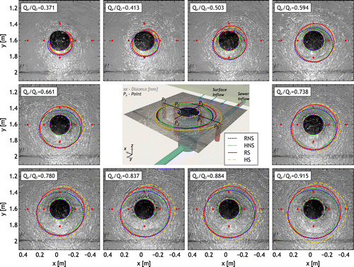
Based on the observations of the extent and shape of the numerical jump around the manhole (see Figure 3), the tests can be classified into three groups (G):

•	G1 In this group (0.37 < Qe/Q1 < 0.5) the sewer surcharge Qe is less than half the magnitude of the main flow Q1. For these tests, Qe appears to be dominated by the main flow since the supercritical region around the manhole is not entirely circular. The numerical models predict a crescent shaped jump, which is in good agreement with the experimental observations. The skewed boundary conditions provide a better fit. Although RS contour is not as crescent-shaped as the others, its jump extent is similar. This effect can be attributed to the different type of mesh discretisation at the manhole, since this effect is not observed in the HS.
•	G2 In this group (0.5 < Qe/Q1 < 0.8) the surcharging flow Qe becomes strong enough to form a fully closed supercritical zone around the manhole, as replicated by all the numerical models. At the measurement points closest to the manhole (in particular P2) subcritical flow is observed, which means that the influence from the surface inflow remains significant.
•	G3 In this group (0.8 < Qe/Q1<0.92) the surcharging flow Qe entirely dominates the surface flow in the vicinity of the manhole to the point that supercritical flow spans all those transducers that are located within 90[mm] from the manhole borderline (see Figure 3).

The numerical models’ behaviour shown in Figure 3 indicate a regime transition from subcritical to supercritical across the circular edge of the manhole, and from supercritical to subcritical around the manhole, also shown by the observations. Around the manhole, the surcharged flow leads to the formation of an approximately circular, slightly skewed, hydraulic jump. Figure 3 also shows that the centre of the hydraulic jump is slightly dislocated given the influence of the main inflow, the floodplain bed and the skewed inflow. Therefore, the solvers with the skewed boundary conditions (i.e. RS and HS) provided a better match with the experiments as compared to the model predictions based on the non-skewed boundary condition.

The influence of the mesh type is also visible in the predicted shape of the hydraulic jump. The HLLC variants tend to form a jump shape that resembles a rounded rectangle, mostly due to their quadrilateral meshes. In contrast, the flexibility of the triangular meshing tends to better capture the circular shaping of the jump. Another mesh dependent difference is the subcritical to supercritical transition across the edge of the manhole. Here, for both inflow boundary condition settings, RNS vs RS, and HNS vs HS produced the same calculation for the transcritical contour. However, a difference between the Roe and HLLC solvers can be addressed to the different mesh discretisations at the edge of the manhole (see zoomed-in portions in Figure 1). As seen in the figure, the triangular mesh favours better alignment with the manhole’s curvature, whereas cut-cells are unavoidable for the quadrilateral mesh. Overall, the location of the predicted hydraulic jump is in good agreement with the experimental observations, especially when the skewed boundary condition is applied.

Hydraulic head

Figure 4 compares the experimental heads, as measured by the transducers (see central sub-figure in Figure 4), with the depths calculated by the numerical models each taken with the skewed and non-skewed inflow boundary conditions. The six sub-figures illustrate the comparisons relative to each measurement point. The experimental heads are included in terms of averages of time series and their variations up to the bounds defined by the 1st and 3rd quartile of the data obtained from the transducers. The relative L₂ norm (Equation (11(11) )) and the aggregated L₁ difference (AL₁ in Equation (12(12) )) are used to assess the differences between the numerical models and the averaged experimental data across all tests.(11) (12)

•	P0 is situated [0, 0.195] [m] relative to the manhole centre. At P0, HS produces the closest match to the experimental data. For all Qe, the HLLC variant predictions (i.e. HS and HNS) generated the smallest error (see Table 1) and remain within the bound of the experimental data. In contrast, for Qe = 3.38[l/s], the calculations of RNS and RS solvers are slightly outside the range of the experimental data, which is ±2 [mm]. One possible reason for this discrepancy is that when Qe = 3.38[l/s] the hydraulic jump is situated close to this measurement point hence producing comparatively large oscillations in the experimental data. However, the discrepancy is only 3 [mm] and does not occur with the HLLC solvers. For Qe > 3.77[l/s], there is a close overlap between the prediction delivered by all the models (i.e. RNS = RS and HNS = HS). For these tests, the flow is supercritical at the transducer due to a relatively bigger magnitude of Qe, which eliminates the influence from the main floodplain flow Q1. For Qe ≤ 2.86[l/s], the opposite is observed as the flow is mainly dominated by Q1, which leads to subcritical flow prevailing at this location.
•	P1 is located [0, 0.395] [m], relative to the manhole centre. At this point, all model predictions are in subcritical flow regime for the full range of Qe considered. The results among the models are seen to be very close, with differences lower than 1.5 [mm], and inside the range of experimental data. All models show a minor underestimation. In terms of L2 error, the solvers which use the skewed boundary condition have the smallest errors. This may be due to P1 location at the side where (within the skewed boundary set up) the highest inflow occurs. P2 is located upstream of the manhole (i.e. [0.210, 0] [m] relative to the manhole centre), and is the most affected by the main inflow Q1. This point presents the largest discrepancy between numerical calculations and experimental data. At this point and irrespective of the mesh type, the models with the non-skewed inflow boundary condition fall outside the range of the measurements. For Qe ≤ 4.46[l/s], models over-predict depths, thus are likely to provide unreliable predictions of the hydraulic jump location for these sewer overflows. HNS and RNS predict supercritical flow when Qe = 4.46[l/s] and Qe = 4.77[l/s], respectively; whereas HS and RS predict its presence more accurately for Qe = 3.77[l/s]. Here, RS and HS best reproduce the experimental data, despite showing local discrepancies for the two cases involving the highest sewer outflow. The comparative results at this position suggest that the smaller the magnitude of the sewer outflow, the more care is required to account for the directional (floodplain) inflow within the models.
•	The point P3 ([−0.210, 0] [m] relative to the manhole centre) is located along the direction of the main floodplain flow but downstream of the manhole. It is under the combined influences of the flow surcharging from the manhole and the main subcritical flow over the floodplain. For Qe < 2.4[l/s] (i.e. in Qe = 2.11[l/s] and Qe = 2.35[l/s]), all numerical models underestimate the measurements, while remaining consistently subcritical. For Qe = 2.86[l/s], the models show a high discrepancy with the measurements. As these discrepancies are apparent within all models, they can be attributed to the complex 3D nature of the flow at this point where main and sewer overflow interact. Also, local geometric imperfection in the physical model could contribute to these discrepancies for 2.11[l/s] ≤ Qe ≤ 2.86[l/s], where the magnitude of Qe is not strong enough to produce supercritical flow around the manhole. In contrast, for the higher surcharging flow, all models closely predict the location where supercritical flow becomes established. For these cases, both Roe solvers appear to deliver closer agreement with experiments relative to the HLLC variants. Since the skewness of the inflow has no influence, this improvement in performance among the solvers is speculated to be due to the geometric flexibility of the triangular mesh (on which the Roe solvers are implemented), which offered a better capture of the surcharged flow and the circular jump. Nonetheless, the cut-cells and directional effects induced by the quadrilateral mesh HLLC solvers have little influence, i.e. a discrepancy in the magnitude of 0.0125 [m]. Looking at the L2 at this point, considering all cases, the HS model generates a slightly smaller error than the other models.
•	At P4, located [0, −0.195] [m] relative to the manhole centre, for Qe ≥ 3.77[l/s] all models lead to very good agreement with the measurements and the mesh-type effects reported previously for P3 are reduced. This again indicates that when the surcharge from the manhole is dominant, the influence of the mesh type and the inflow from the floodplain become less influential (apart for Qe = 3.38[l/s] where HNS slightly underperforms). For lower sewer outflows, differences in behaviour between the models are noted. In particular, for Qe = 2.86[l/s], the HS and RS models under-predict the measurements suggesting a supercritical flow. The RNS model also predicts supercritical flow and is closer to the experimental head. In contrast the HNS model incorrectly predicts subcritical flow. It should be noted that, for this test (i.e. Qe = 2.86[l/s]), there is a higher uncertainty in the measurement since the hydraulic jump was oscillating above this transducer. For smaller Qe, the models associated with the non-skewed boundary condition perform better relative to the experiments than their skewed inflow variants. Quantitatively, RS, HNS and HS generate roughly the same error magnitudes. The error provided by the RNS solver is approximately 50% less than the others, associated with a better prediction for Qe = 2.86[l/s].
•	The point P5 is located [0, −0.395] [m] relative to the manhole centre. Unlike at all the other points, the results produced by RNS and HNS (i.e. with non-skewed boundary condition) are globally closer to the measurements compared to their skewed variants (RS and HS). Here, the skewed inflow condition seems to have reduced the flow, and therefore the depth predictions. Moreover, the HS solver leads to increased divergence from the measurements with increasing surcharge, leading to an incorrect prediction of supercritical flow for the highest Qe . Since this behaviour is not observed with RS predictions on the triangular mesh, it is likely to be due to the reduced flexibility of the quadrilateral to directly handle 45º-skewed flow. In terms of L2, at this point, RNS and HNS have very minor errors, which are the smallest across all points and tests considered. Therefore, irrespective of the mesh-type and the inflow boundary condition, first-order solvers appear to be generally valid for modelling of sewer-to-floodplain flow when not concerned with modelling details in the local vicinity of the manhole.

Figure 4. Comparison between the experimental observations and numerical hydraulic heads at each measurement location. The (temporally averaged) experimental data points are bounded by the 1st and 3rd quartile of the measured time series data.

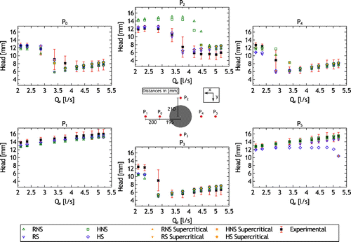
Table 1. Relative L₂ norm and the aggregated L₁ difference (AL₁), used to assess the differences between the numerical models and the averaged experimental data across all tests.

Model	L2[−]						AL1 [m]
	P0	P1	P2	P3	P4	P5
RNS	0.144	0.068	0.518	0.212	0.076	0.014	0.0013
RS	0.130	0.043	0.101	0.192	0.158	0.057	0.0008
HNS	0.072	0.049	0.407	0.190	0.132	0.015	0.0011
HS	0.066	0.044	0.139	0.188	0.135	0.167	0.001

Taken as a whole, the numerical models are able to provide a good representation of the experimental observations, in most cases within the range of expected measurement error. This is in spite of the stated boundary condition uncertainties as well as the inherent hydrostatic pressure assumption and 2D depth-averaged nature of the models. In terms of aggregated absolute difference between numerical models prediction and experiments, it is found to be 1.05 [mm] overall; RS and HS present the smallest difference (i.e. 0.8 [mm] and 1.0 [mm] respectively) while RNS and HNS presented the highest (i.e. 1.3 [mm] and 1.1 [mm]).

Summary and conclusions

This work has been motivated by the need to experimentally validate this modelling formulation when the floodplain flow is locally affected by a shock-wave arising from the impact of a surcharging manhole. Two popular FV-based flood models have been selected for this purpose. The first employs the Roe solver on an unstructured triangular mesh, and the second uses the HLLC solver on structured quadrilateral mesh. Experimental measurements were obtained from a physical model, linking a slightly inclined urban floodplain to the sewer system via a manhole. The experimental tests were conducted under steady state flow conditions for a series of increasing surcharge sewer flows (Q_e). The numerical models have been modified to fit the physical flow and geometrical conditions of the floodplain. These modifications considered local mesh refinement around the manhole area, an additional source term in the SWE to incorporate sewer overflow (Q_e) into floodplain flow, and weighting of the inflow boundary condition (Q₁), i.e. in a quasi-2D manner (skewed inflow). The performance of these numerical models is explored against measurements taken around the manhole. Their ability to locate the circular jump has been qualitatively evaluated by superimposing critical Froude number estimations against observed experimental jump behaviour. More in-depth validation is performed by assessing their reproducibility against hydraulic heads measured by six transducers located around the manhole.

In terms of localisation of the circular jump around the manhole, the predictions amongst the models with the skewed (i.e. RS and HS) vs the non-skewed (i.e. RNS and HNS) inflow tend to increasingly deviate with increasing sewer-to-floodplain flow ratio, Q_e/Q₁. The choice of mesh appears to further contribute to increase the modelling discrepancies (i.e. among RS and HS models). The combined effect of the skewed floodplain inflow and the preferential directions of the quadrilateral mesh (i.e. with HS) produced the widest supercritical flow area, as compared with any of the other models. However, this effect was mainly present for high overflow rate and, therefore, could be associated to the uncertainty on the weighting of the skewed inflow boundary condition. However it should be noted that absolute errors cannot easily be attributed to either the spatial discretisation, or the Riemann solver given they are not tested independently.

More detailed comparison of these model predictions against the measured hydraulic head seems to indicate that their level of reliability can be associated to the sewer-to-main flow ratio, Q_e/Q₁. When the sewer overflow Q_e was strong enough to generate the circular water jump, Q_e/Q₁ > 0.65, all models could predict the measurements with no special treatment. In contrast, the main inflow Q₁ seems to be influential for relatively weaker Q_e . In these cases, RS and HS closely reproduce the measured hydraulic head at the measurement positions located at the side of the skewed inflow Q₁, where the floodplain flow is higher. From the other side, RNS and HNS outperformed. This implies that the sensitivity of these models may increase with decreasing Q_e/Q₁ ratio, and therefore require more calibration from the user especially when concerned with localised modelling of sewer-to-floodplain flow. Nonetheless, the reproducibility of all the models to the experiments is very good outside the range of the circular jump, especially when not applying the skewed inflow boundary treatment.

From the steady state tests considered, FV 2D shock capturing flood models (including Roe and HLLC) are valid approaches to replicate the hydrodynamics of sewer-to-floodplain flow either when sewer-outflow is strong enough to induce a circular jump or when the surface flow is dominant.

Disclosure statement

No potential conflict of interest was reported by the authors.

Supplemental data

Supplemental data for this article can be accessed at http://dx.doi.org/10.1080/1573062X.2017.1279193 and http://www.sheffield.ac.uk/polopoly_fs/1.679303!/file/Validationof2Dshockcapturingfloodmodels.xlsx.

Funding

The research was supported by the UK Engineering and Physical Sciences Research Council [EP/K040405/1].

References

- Borsche, R. and Klar, A., 2014. Flooding in urban drainage systems: coupling hyperbolic conservation laws for sewer systems and surface flow. International Journal for Numerical Methods in Fluids, 76, 789–810. doi:10.1002/fld.3957.
- Cea, L., Garrido, M., and Puertas, J., 2010. Experimental validation of two-dimensional depth-averaged models for forecasting rainfall runoff from precipitation data in urban areas. Journal of Hydrology, 382, 88–102. doi:10.1016/j.jhydrol.2009.12.020.
- Chen, A., et al., 2015. Modelling sewer discharge via dis- placement of manhole covers during flood events using 1D/2D SIPSON/P-DWave dual drainage simulations. Urban Water Journal, 13 (8), 530–840. doi:10.1080/1573062X.2015.1041991.
- Chow, V.T., 1959. Open-channel hydraulics. New York: McGraw-Hill.
- Djordjević, S., et al., 2005. SIPSON- simulation of interaction between pipe flow and surface overland flow in networks. Water Science & Technology, 52 (5), 275–283.
- Falconer, R.H., et al., 2009. Pluvial flooding: new approaches in flood warning, mapping and risk management. Journal of Flood Risk Management, 2 (3), 198–208. doi:10.1111/j.1753-318X.2009.01034.x.
- Hager, W.H., 2010. Wastewater Hydraulics. Berlin, Second Edition: Springer.10.1007/978-3-642-11383-3
- Kesserwani, G., and Wang, Y., 2014. Discontinuous Galerkin flood model formulation: Luxury or necessity? Water Resources Research, 50, 6522–6541. doi:10.1002/2013WR014906.
- Leandro, J., Chen, A., and Schumann, A., 2014. A 2D parallel diffusive wave model for floodplain inundation with variable time step (P-DWave). Journal of Hydrology, 517, 250–259. doi:10.1016/j.jhydrol.2014.05.020.
- Leandro, J., Schumann, A., and Pfister, A., 2016. A step towards considering the spatial heterogeneity of urban key features in urban hydrology flood modelling. Journal of Hydrology, 535, 356–365. doi:10.1016/j.jhydrol.2016.01.060.
- Lee, S., et al. (2013), Experimental Validation of Interaction Model At Storm Drain for Development of Integrated Urban. Journal of Japan Society of Civil Engineers, Ser. B1 69(4), 109–114. doi:10.2208/jscejhe.69.I_109
- Mahdizadeh, H., Stansby, P.K., and Rogers, B.D., 2012. Flood Wave Modeling Based on a Two-Dimensional Modified Wave Propagation Algorithm Coupled to a Full-Pipe Network Solver. Journal of Hydraulic Engineering, 138 (3), 247–259. doi:10.1061/(ASCE)HY.1943-7900.0000515.
- Martins, R., Leandro, J., and Djordjević, S., 2015. A well balanced Roe scheme for the local inertial equations with an unstructured mesh. Advances in Water Resources, 83, 351–363. doi:10.1016/j.advwatres.2015.07.007.
- Martins, R., Leandro, J., and Djordjević, S., 2016. Influence of sewer network models on urban flood damage assessment based on coupled 1D/2D models. Journal of Flood Risk Management. doi:10.1111/jfr3.12244
- Neal, J., et al., 2012. How much physical complexity is needed to model flood inundation? Hydrological Processes, 26 (15), 2264–2282. doi:10.1002/hyp.8339.
- Néelz, S., and Pender, G., 2012. Benchmarking of 2D hydraulic modelling packages - tuflow, Technical Report June, Environment Agency, Bristol.
- Nikolos, I., and Delis, A., 2009. An unstructured node-centered finite volume scheme for shallow water flows with wet/dry fronts over complex topography. Computer Methods in Applied Mechanics and Engineering, 198 (47-48), 3723–3750. doi:10.1016/j.cma.2009.08.006.
- Rubinato, M., (2015). Physical scale modelling of urban flood systems. Phd thesis. University of Sheffield.
- Schöberl, J., 1997. NETGEN an advancing front 2D/3D-mesh generator based on abstract rules. Computing and visualization in science, 1 (1), 41–52. doi:10.1007/s007910050004.
- Seyoum, S., et al., 2012. Coupled 1D and noninertia 2D flood inundation model for simulation of urban flooding. Journal of Hydraulic Engineering, 138 (1), 23–34. doi:10.1061/(ASCE)HY.1943-7900.0000485.
- Smajstrla, A.G., Harrison, D.S., and Zazueta, F.S. (1985). Agricultural water measurement. Intitute of Food and Agricultural Sciences, Bulletin. Gainesville: University of Florida, 207
- Toro, E.F., Spruce, M., and Speares, W., 1994. Restoration of the contact surface in the HLL- Riemann solver. Shock Waves, 4 (1), 25–34. doi:10.1007/BF01414629.
- Wang, Y., et al., 2011. A 2D shallow flow model for practical dam-break simulations. Journal of Hydraulic Research, 49 (3), 307–316. doi:10.1080/00221686.2011.566248.
- Zhao, C., Zhu, D., and Rajaratnam, N., 2004. Supercritical sewer flows at a combining junction: A model study of the Edworthy trunk junction, Calgary, Alberta. Journal of Environmental Engineering and Science, 3 (5), 343–353. doi:10.1139/s04-019.
- Zhao, C., Zhu, D., and Rajaratnam, N., 2006. Experimental Study of Surcharged Flow at Combining Sewer Junctions. Journal of Hydraulic Engineering, 132 (12), 1259–1271. doi:10.1061/(ASCE)0733-9429(2006)132:12(1259).