Robust optimization of valve management to improve water quality in WDNs under demand uncertainty

ABSTRACT

Water quality deterioration in water distribution networks can be associated with high water residence time in the network. To this end, some previous studies have proposed optimization procedures for valve management. However, these studies generally come up with operational configurations assuming deterministic user demand patterns that may never occur in reality. In consequence, the proposed solutions may not be effective for improving water quality or do not comply with pressure constraints if different demand patterns are observed. This study proposes a methodology to determine robust configurations of the valves to keep water residence time at acceptable levels regardless of the variability in demand patterns. The methodology is tested on four different distribution systems of varying topology and size. Results show the importance of executing robust – instead of deterministic, optimization to find valve configurations that guarantee the performance of the networks in terms of hydraulics and water quality.

KEYWORDS:

• Robust multi-objective optimization
• water age
• demand uncertainty

Introduction

Many water quality problems in Water Distribution Networks (WDNs) can be associated with high water residence time in the system, known also as water age. Indeed, high water age affects several physical, biological and chemical aspects, contributing to the accumulation of sediments in pipes, corrosion, undesirable odours and stimulation of chemical reactions (Association, American Water Works 2002; Machell and Boxall 2014; Machell et al. 2009; Masters et al. 2015). Besides, chlorine residual concentration decreases with age, impacting its efficiency as a purifier. In distribution systems where chlorine is used as disinfectant, high water age also facilitates the generation of disinfection by-products (DBPs) such as trihalomethanes (THMs), which are carcinogenic (e.g. Morris et al. 1992; Weinberg et al. 2002). For these reasons, water age is often taken as a global indicator of water quality in WDNs (Fu et al. 2012; Shokoohi et al. 2017), implying that a well-performing WDNs should keep water age in the network at low values.

The main factors contributing to increase water age are the design of WDNs to cope with future demand based on an estimated growth of the population, possible commercial and industrial developments, and fire protection. For example, in the first years of operation the networks may be oversized for the reduced water demand in comparison to the design demand; the same can happen if the projections of population growth or developments used in the design do not occur as foreseen.

Proper operational interventions, including valve management, can be achieved by means of optimization procedures. Optimization has been applied to solve a range of problems related to the design and operation of WDNs and a comprehensive review is reported by Mala-Jetmarova, Sultanova, and Savic (2017).

Several studies have proposed the optimization of valves’ operations to improve water quality. Among the existing studies, Prasad and Walters (2006) suggested to minimize water age by finding optimal operational valves status using a single-objective optimization problem formulation solved with genetic algorithms. More recently, Quintiliani et al. (2017) and Quintiliani et al. (2019) addressed the same problem using a multi-objective optimization formulation, in which both the water age and the number of operational interventions are minimized. Although Abraham, Blokker, and Stoianov (2017) used valve management to maximize the self-cleaning capacity of the network to decrease the risk of discolouration during the peak hours of demand using a single objective optimization. Other authors have proposed the optimization of valves’ configuration by minimizing operational costs. Carpentier and Cohen (1993) optimized the scheduling of valves by the decomposition and coordination of local problems using discrete dynamic programming . Optimal scheduling of valves, among other network elements, has been solved using augmented Lagrangian method (e.g. Ulanicki and Kennedy 1994) and using decomposition, using the projected gradient and the complex methods (e.g. Cohen, Shamir, and Sinai 2000a, 2000b, 2009).

Most of these studies, however, neglect that the behaviour of the network can be affected by uncertain parameters or design variables. It is well known that these uncertain inputs can affect the estimation of hydraulic and chemical processes that are mainly model-based (Di Cristo, Leopardi, and de Marinis 2015; Idornigie et al. 2010; Pasha and Lansey 2005). As a consequence, the solutions obtained from a model-based optimization are also affected by uncertainty in the parameters. Water demand is one of the main recognised sources of uncertainty. Several works have aimed at the minimization of cost and the maximization of WDN robustness or resilience taking into account the uncertainty of water demands. Babayan, Savic, and Walters (2004) used the multi-objective optimizer NSGA-II where, in every stage of the evolution, uncertain parameters are used to identify critical nodes and the most significant variables impacting resilience. Kapelan, Savic, and Walters (2005), Kapelan et al. (2006) and Savic (2006) used robust NSGA-II (rNSGA-II) as the multi-objective optimizer, which takes into account uncertainty in the evaluation of the objective functions. To select a robust solution during the evolution of the algorithm, the uncertainty is incorporated carrying out a small number of samples of the uncertain parameters.

The few researches associated with reducing water age via valve management (Prasad and Walters 2006; Quintiliani et al. 2017; Quintiliani et al. 2019) use a deterministic approach assuming a ‘representative’ daily demand pattern without considering uncertainty. This is a limitation because the uncertainty in water demand affects the hydraulic conditions, impacting water age in the network. The novelty of this study is to improve the method presented by Quintiliani et al. (2017) and Quintiliani et al. (2019), proposing a methodology for realizing a robust optimization, which considers demand uncertainty. To this end, the Loop for Optimal valve status Configuration (LOC) algorithm is used in combination with RObust optimization and Probabilistic Analysis of Robustness (ROPAR), which is explained in the next section (for other cases using ROPAR see Marquez-Calvo and Solomatine (2019)). In this paper, four different networks of varying sizes and complexities are used to demonstrate the appropriateness of the methods, comparing both deterministic and robust optimization results.

The rest of this paper is structured as follows: first, the methodology is presented, in which the optimization problem is formulated and where details about deterministic and robust optimization using ROPAR are presented. The methodology also presents the experimental design and the proposed criteria to compare both methods. Next, the four water distribution networks are presented and described, followed by the presentation, analysis and discussion of results. Finally, conclusions and recommendations are presented.

Methodology

Description of the optimization problem

The problem consists of robustly minimizing the water age in a network by operating a convenient set of valves, in such a way that the water age stays as close as possible to its minimum value knowing that water demand is uncertain. We assume that every pipe in the network has a potential shut off valve to be operated. The decision variables are the statuses of the valves, represented in principle by binary values (open or closed). Further investigations will consider degrees of valve closures or openings as suggested by Kang and Lansey (2009) and Ostfeld and Salomons (2006).

The multi-objective optimization problem considers two objective functions: the water age, evaluated as the Demand weighted Mean Water Age (DeMeWA, Equation (1)) and the Number of valve Closures (NoC, Equation (2)):

(1) $ObF1=\underset{\mathit{x}}{min}DeMeWA\left(\mathit{x},u\right)=\underset{\mathit{x}}{min}\frac{{\sum }_{i=1}^D{\sum }_{t=0}^{T}W{A}_{i,t}\left(\mathit{x},u\right)\ast q_{i,t}}{{\sum }_{i=1}^D{\sum }_{t=0}^T{q}_{i,t}}$(1)

(2) $ObF2=\underset{\mathit{x}}{min}NoC\left(\mathit{x},u\right)$(2)

WA_i,t is the water age at the i-th node at time step t; D is the number of demand nodes in the network, T represents the number of time steps within the Total Simulation Time (TST); q_i,t is the water demand requested at node i at time step t. NoC represents the number of valves that have been intervened (closed); x is the vector of decision variables, containing one of two possible values for each pipe in the network: 1 if the valve is open and 0 if it is closed. Furthermore, u is a vector containing demand pattern factors (24 positive values, one per hour of the day), which are the uncertain parameters.

Two constraints are needed to guarantee that: 1) any valve configuration status delivers water to all nodes, i.e. nodes cannot be disconnected; 2) the pressure P_i,t in each node i at each time t must be within a fixed, acceptable range:

(3) $P_{min}\le P_{i,t},\left(\mathit{x},u\right)\le P_{max}\mathrm{\forall }t=\mathrm{0..}T\mathrm{\forall }i=\mathrm{1..}D$(3)

It is worth noting that the objective functions and the constraints depend on both the decision variables and the demand pattern.

To calculate the value of the objective functions and constraints, a computer program was developed. The program incorporates the valve configurations in the input file of the hydraulic model and, using the EPANET Programmer’s Toolkit (Rossman 1999), run the hydraulic and water quality engines. To verify the existence of disconnected nodes, the error thrown by EPANET is checked. For the evaluation of water age, complete mixing at nodes is assumed and dispersion is neglected (Boccelli et al. 1998; Di Cristo and Leopardi 2008).

Deterministic optimization (DO)

To perform the deterministic optimization, a fixed 24 hours demand pattern is considered in each node. The LOC algorithm is a fast procedure to quickly find sub optimal solutions. LOC is a greedy algorithm (e.g. Alfonso et al. 2013; Banik et al. 2017) that works by stages. In the first stage, with all valves of the network open, the LOC algorithm closes one pipe at a time in order to find the one that offers the highest reduction in ObF1. In the second stage, the pipes that were not selected in the first stage are, again, closed one at a time, keeping the valve selected in the first stage closed, and finding in this way the second pipe that gives the highest reduction in ObF1. This process is repeated until one of the constraints is violated (either disconnection or minimum pressure).

Robust optimization using ROPAR

Robust optimization (RO) of multiple objectives is an optimization method that generates a set of optimal solutions that offers the smallest variability of the objective functions when some elements or parameters of the modelled real system are varying due to their uncertainty (e.g. Deb and Gupta 2006; Erfani and Utyuzhnikov 2012; Gaspar-Cunha and Covas 2008; Gunawan and Azarm 2005).

For the considered problem, the objective is to obtain a robust configuration of valves, such that minimizes water residence time and keeps it near its minimum even under a large range of possible user demands.

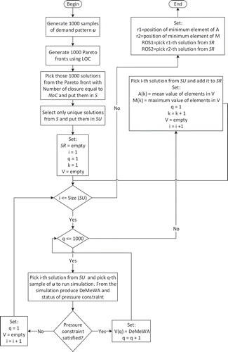
To find robust solutions, the ROPAR algorithm is adopted (Marquez-Calvo and Solomatine 2019). ROPAR is applied to this case in three parts, namely I) demand pattern sampling and generation of Pareto fronts, II) analysis of Pareto fronts and III) selection of the robust solution.

Part I. Demand pattern sampling and generation of Pareto fronts

Because demand node variability is related to the behaviour of each user then it is a stochastic process (e.g. Blokker, Vreeburg, and Van Dijk 2009). In a stochastic representation of this process the values of the uncertain parameters (in our case a set of hourly pattern multipliers), are produced with a Monte Carlo sampling obtaining n different water demand patterns. To generate these uncertain multipliers, the historical mean demand, named m_base,k, is used as a base. The m stands for multiplier. The sub-index k indicates the hour of the day (i.e. 1 to 24) the multiplier is applied to. To perform the sampling, the daily variability of residential water demand is simulated, considering two different probability distributions: Normal and Log-Normal (Tricarico et al. 2007). For both probability distributions, the m_base,k is the base demand (i.e. the value used for the DO) and the standard deviation is assumed 20% of the base demand, both base demand and its standard deviation obtained from historical demand. In particular, if the base demand is less than 1.5, the Normal distribution is considered; otherwise the Log-Normal distribution is adopted. The uncertain demand is named m_uncertain,k, which is modelled as an independent random variable obtained from the distributions mentioned above and represented in Equation (4).

(4) $m_{uncertain,k}\sim \left\{\begin{array}{c}Normal\left(m_{base,k},{0.2}^2\right),if{m}_{base,k}<1.5\\ Log-Normal\left(m_{base,k},{0.2}^2\right),if{m}_{base,k}\ge 1.5\end{array}\right.$(4)

For convenience u is defined as the vector [m_uncertain,1, m_uncertain,2, …, m_uncertain,24]. If the networks are in residential areas, only one vector u is necessary to represent the domestic demand of all nodes in the network, and in this case 24 random variables are considered. If the networks have m different demand patterns, then m number of vectors u would need to be generated, and the number of random variables would be 24*m.

A common assumption from the modelling perspective (e.g. (Abraham, Blokker, and Stoianov 2017; Blokker, Vreeburg, and Van Dijk 2009)) is that the demands from individual households or connections with similar demand type are aggregated and assigned to a node that represents such an area. In this paper we also follow this assumption, and therefore small pipes connecting the households to the distribution network are not modelled.

Latin Hypercube sampling is used as the method for Monte Carlo analysis. In this paper we sample n = 1000 demand pattern vectors u. For each pattern, the optimization problem is solved using LOC, obtaining 1000 Pareto-quasi optimal sets.

For the process just described, the sampling confidence (i.e. SC) can be calculated, which is defined as the percentage of the sample space explored. This SC is dependent on the confidence level of each of the 24 random variables. The formula relating these concepts is:

(5) $SC\left(\mathit{u}\right)=\prod _{k=1}^{24}confidencelevel(m_{uncertain,k})$(5)

Part II. Analysis of Pareto fronts

In this step the family of n Pareto fronts obtained in part I are analysed. The analysis consists of identifying the value of one objective function for which the value of the other objective function yields the lowest possible variance. In our case, we aim to identify the value of ObF2 (i.e. NoC) that yields the lowest variance for ObF1 (i.e. DeMeWA). To this end, first an initial NoC value is selected; second, all (n) corresponding values of DeMeWA are extracted from the Pareto fronts, and stored in set S. Third, an empirical probability distribution is built with the values in S, obtaining an approximation of the probability density function characterizing DeMeWA for that initial NoC. Finally, the procedure is repeated for different values of NoC, selecting at the end the one that gives the minimum DeMeWA variance.

Part III. Selection of the robust solution

This step consists of two main parts. First, check if S contains repeated solutions; if so, then eliminate them in order to obtain a set of unique solutions S_U. Each unique solution might have associated a number r of repeated solutions. This number r is the frequency of the unique solution. This frequency of the unique solution is used in the analysis of results.

Second, find a network configuration that works for every possible demand pattern generated, as it is explained next. Take the first value in S_U and retrieve its associated network configuration. For each generated demand pattern u, run the retrieved network and obtain its DeMeWA value. If one or more demand patterns generate violations of the pressure constraint, it is said that the network is not reliable and must be discarded; otherwise, this (reliable) network is stored in the set S_R. For each network in S_R, the mean and maximum of DeMeWA (over the n demand patterns) are calculated. Repeat the procedure for the rest of the network configurations associated to the values in S_U. At the end, a set of reliable solutions S_R of cardinality R is obtained. Note that R can be less or equal to the number of Pareto fronts originally generated (R ≤ n). In addition, two vectors of size R, containing the averages (i.e. A) and the maxima (i.e. M) of DeMeWA are obtained.

Two criteria of robustness are considered: the network that gives the minimum average of DeMeWA (i.e. ROS1 = min(A)), and the minimum maximum of DeMeWA (i.e. ROS2 = min(M)). Note that the robust network obtained with ROS1 can be different from that obtained with ROS2. If ROS1 is different from ROS2 it is not possible generalize that ROS1 is always better than ROS2 nor vice versa. The selection of one of these two solutions is going to depend on the analysis of the trade-offs of one against the other, a decision that is left to the decision maker.

Furthermore, it is worth mentioning that the minimum maximum DeMeWA is not looking for a solution that complies with a specific threshold. What the method is looking for is a solution with the minimum worst case.

The three parts of the method are presented in Figure 1. In this figure, V is a vector storing the 1000 values of the DeMeWA result of evaluating one single solution with each of the 1000 samples of user demand.

Figure 1. Flow chart of the method.

Assessing the total reliability

We now introduce the concept of total reliability (i.e. TR) of a network. This parameter indicates the minimum performance that we can expect from the network. To calculate TR, the reliability of the solution is required.

The reliability (i.e. R) of a solution is the ratio between the number of samples where the solution complies with the constraint of the network (i.e. minimum pressure for every node) and the total number of samples. It can be represented with the following equation:

(6) $R=\frac{numberofsampleswheresolutioncopes}{totalnumberofsamples}$(6)

So far two concepts related with probability have been mentioned, SC and R. These two concepts are used to define the TR of the network. The multiplication of the R of a solution with the SC of the sample used defines the TR of the network.

(7) $TR=SC\ast R$(7)

Experimental setup

The methodology is applied to four different water distribution systems, introduced in the next section, and for each of them ROS1 and ROS2 are compared. In addition, the networks are solved using deterministic optimization, and the solution (i.e. DOS) is evaluated over the set of n demand patterns as a baseline for comparison.

Computational complexity

There are two algorithmic parts in the proposed method. The first part is the execution of LOC and the second part is the number of times that LOC is repeated to take into account the uncertainty.

First, the complexity of LOC is analysed. As it can be inferred from its description, LOC uses a limited number of function evaluations to find a Pareto front, understanding as one function evaluation one execution of EPANET. The number of function evaluations is therefore, (Equation (8)).

(8) $E=\sum _{i=N}^{P}i$(8)

Where E is the number of function evaluations, P is the number of pipes of the network and N is the number of nodes. The result of this expression is 0.5*[P² + P-N² + N]. Therefore, obtaining a Pareto front using LOC requires polynomial time.

In the second part the LOC algorithm is repeated for the number of the considered samples, which in this paper is 1000 regardless of the network. The number of function evaluations per network is 1000*0.5*[P² + P-N² + N]. Note that the order of this expression is still polynomial.

An advantage of using this method is the possibility to run each of these 1000 executions of LOC in parallel, thus, having the possibility of obtaining the results in the time required by just one execution of LOC if there are 1000 CPUs available.

In this paper, 1000 samples were used. However, in general, the number of samples of u depends on two factors, the number of random variables and the size of the network. A reflection is presented in the section of results about the number of samples.

Description of the water distribution systems used for analysis

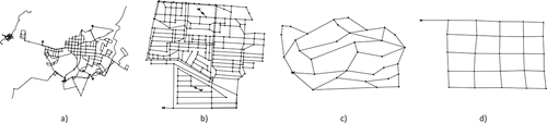
Four distribution systems from the literature, representing residential areas, are used to test the methodology. They are named in this paper as Sys473 (Jolly et al. 2013), Sys365 (Alfonso, Jonoski, and Solomatine 2009), Sys47 (Prasad and Walters 2006) and Sys40 (Alfonso, Jonoski, and Solomatine 2009). The number that follows the ‘Sys’ prefix indicates the number of potential valves to be operated in each network. Their schemes are shown in Figure 2. Topology, geometric data, base demand and pattern values are the same as reported in the original papers, and not repeated herein.

Figure 2. Scheme of the cases of study: a) Sys473, b) Sys365, c) Sys47 and d) Sys40.

In each considered system, all demand nodes have the same base demand and a one-hour time step pattern. The DO is carried out considering the ‘base’ demand pattern, while in the RO, the multipliers are modified within a Monte Carlo method, as described in the methodology. For each pattern, hydraulic and quality simulations are performed with a time step equal to five minutes. The DeMeWA values (i.e. Equation (1)) have been calculated on a 24 h period (TST = 24 h). The values used as pressure thresholds in Equation (3) are P_min = 15 m and P_max = 100 m, and they guarantee a demand-driven functioning.

Results

Deterministic optimization results (using LOC)

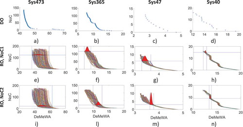
The Pareto fronts obtained with DO for the four networks are shown in the first row of Figure 3. It can be observed that DO allows to have, with an adequate number of closures, a reduction of water age of around 50% of the value corresponding to the ‘do nothing’ option. In evaluating the Pareto front, the ‘do-nothing’ solution, corresponding to NoC = 0, is always included to compare how much DeMeWA improves with respect to the original status. The shape of the Pareto front for network Sys473 indicates that the main reduction in DeMeWA is reached with a limited number of closures, while for the others at least one-third of the valves have to be operated.

Figure 3. Pareto fronts obtained using Deterministic Optimization (DO) and Robust Optimization (RO), for different networks.

Robust optimization results (using ROPAR)

Part I of ROPAR. The second and third rows in Figure 3 also report the 1000 Pareto fronts generated with the RO for each system.

Part II of ROPAR. Although any value of NoC can be selected, two values of NoC have been considered to illustrate the analysis. The first value (NoC1) is the number of valve closures for which solutions are available for all Pareto fronts and the minimum value of DeMeWA is reached. These number of closures are 122, 116, 6 and 15 for the networks Sys473, Sys365, Sys47 and Sys40 respectively (see second row of Figure 3).

The second value (NoC2) is the inflexion point at which an increment in the number of closures does not represent a significant reduction of DeMeWA. These values are 20, 20, 3 and 9 for the networks Sys473, Sys365, Sys47 and Sys40 respectively (see third row of Figure 3).

For the two considered NoC values NoC1 and NoC2, the PDFs of the 1000 DeMeWA values are generated, see the second and third rows in Figure 3. The solutions corresponding to low NoC values have smaller standard deviations than those with higher value, meaning that they have less variability and therefore they offer more robustness. However, solutions with high NoC values provide a high reduction of DeMeWA. This clearly represents a trade-off between having less water age and having less variability. To have more information about this trade-off, it is necessary to carry out the analyses that follow.

Part III of ROPAR. To reduce the computational cost, the analysis over repeated solutions is avoided. Therefore only the group of unique solutions for fixed values of NoC (NoC1 and NoC2) is considered (see Table 1). The number of repeated solutions, which is the complement to 1000 of the unique solutions, decreases with the complexity of the network. The number of repeated solutions is 0% and 16.4% in the Sys473 network for the case NoC1 and NoC2, respectively, while for the smallest Sys40 the repeated solutions are 98.4%, and 99.3% for NoC1 and NoC2, respectively.

Table 1. Metadata of the distribution systems.

	Sys473		Sys365		Sys47		Sys40
	NoC1 = 122	NoC2 = 20	NoC1 = 116	NoC2 = 20	NoC1 = 6	NoC2 = 3	NoC1 = 15	NoC2 = 9
Unique solutions	1000	836	683	39	43	7	16	7
Reliable solutions	176	108	675	39	1	1	1	7
DOS reliability (%)	92.9	94.3	100	100	0	10.7	99.3	100
Sampling confidence(%)	96.11	96.11	96.11	96.11	96.11	96.11	95.09	95.09

Figure 4 furnishes information about the reliability and frequency of the unique solutions. To visually present the information more understandably, for each case, the solutions are first ordered by their reliability and then by their frequency. For example considering the chart Sys365, NoC2 (Figure 4(f)) every one of its 39 unique solutions have 100% reliability and the 39^th solution has a frequency of 358. To simplify the discussion, in the rest of the paper a solution is reliable if its reliability is 100%, otherwise it is unreliable. Table 1 indicates that for the NoC2 case, for networks Sys365 and Sys40, all unique solutions are reliable. For Sys40, considering NoC1 valve closures, only one reliable solution is found. For Sys473 85% of the solutions are not reliable for both NoC values. Finally, only one solution is reliable for Sys47 for both NoC values. These results suggest that the number of reliable solutions is influenced by the NoC value and it cannot be correlated to the size of the network. That is, the number of reliable solutions depends essentially on the functioning of the scheme corresponding to the considered number of closures. The analysis indicates also that the deterministic approach gives solutions that cannot cope with the variability of the demands.

Figure 4. Reliability and frequency of unique solutions.

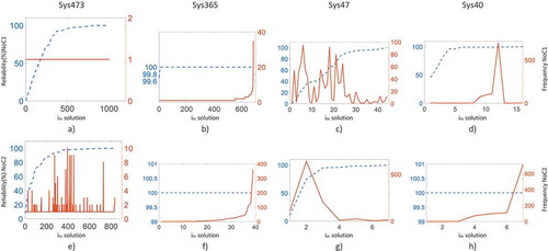
From the reliable solutions, the most robust ones are selected using the criteria ROS1 and ROS2. Actually because the method is looking for solutions with two criteria of minimum variability, ROS1 and ROS2, a Pareto front of robust solutions could be produced. Figure 5 shows, for each considered case, the comparison of the solution found by criterion ROS1 and ROS2 with respect to the rest of the reliable solutions. In three cases represented in Figure 5(c,d,g) only one reliable solution is found. In another three cases (Figure 5(b,f,h)), ROS1 and ROS2 select the same solution. For the cases reported in (Figure 5(a,e)), different solutions are selected as the most robust from the two criteria. In the case Sys473 and NoC1 (Figure 5(a)), a Pareto front with three robust solutions can be seen. These three solutions dominate all the other solutions. The solution in the middle of these three seems to have a good compromise between ROS1 and ROS2, but ultimately it is left to the decision maker to select one of these three robust solutions. In the case Sys473 and NoC2 (Figure 5(e)), a Pareto front with five robust solutions can be seen.

Figure 5. Comparison among ROS1 (R1), ROS2 (R2), DOS (D), and the rest of the reliable solutions for all the cases.

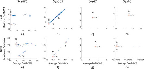
In summary, the results of the RO show that in six of the eight cases the same solution is individuated from both criteria. For the other two cases the ROS1 and ROS2 solutions have a difference of less than 4% with respect to DeMeWA average, while the difference is about 33% with respect to DeMeWA maximum. This result indicates that the ROS2 solution is good in terms of DeMeWA average, while the ROS1 one is not as good as the ROS2 solution considering the DeMeWA maximum. In conclusion, the presented analysis suggests the use of the ROS2 criterion (i.e. the minimum maximum of DeMeWA).

Discussion

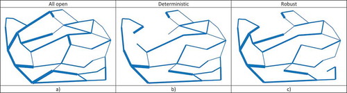
The results of the four networks are analysed next, beginning with the network Sys47. Figure 6 reports the condition with all the valves open and the optimum solutions, deterministic and robust for six pipes closed (i.e. NoC1). In the figure, the thickness of each pipe is proportional to its diameter. The case of the network Sys47 is particularly relevant because the deterministic optimization has 0% reliability (see Table 1). This result remarks the importance of performing a robust optimization, because the implementation of a deterministic solution may have very disastrous consequences on the system functioning. In contrast, the robust solution has 100% reliability. This robust solution stays at a minimum value even when the demand varies. The maximum DeMeWA that this network will have is 3.43 hours and its average DeMeWA will be 3.37 hours (see Figure 5(c)). From these values it is clear that even in the worst case, the DeMeWA will be just 0.06 hours away from the average, or in other words, the solution stays very close to its minimum value regardless of the variation of the demand. For the case of NoC = 3, the deterministic solution has 10.7% of reliability (see Table 1). The robust solution has just a difference of 0.06 hours between the average and maximum DeMeWA, coinciding with the case NoC = 6 about the stability of its solution under variations of the demand.

Figure 6. Network Sys47, all pipes open (a), and optimum solutions closing six pipes (i.e. NoC1), deterministic (b) and robust (c).

The results for the network Sys40 illustrate that a deterministic optimization could find a robust solution for the simplest case of the simplest network (see Figure 5(h)). However there is no way of knowing whether the deterministic solution is indeed robust or not, if not carrying out an analysis considering uncertainty in the demand.

About the network Sys473, there are two important aspects. First point, for both cases analysed (i.e. NoC1 and NoC2), the solutions found by ROS1 and ROS2 are different (see Figure 5(a,e)). However just one of the two solutions has to be adopted. In both cases ROS2 furnishes a better option because these solutions have the minimum value of the maximum DeMeWA and almost the minimum value of the average DeMeWA. Second point, from Figure 4(a,e) it is clear that the number of solutions with 100% reliability is very limited. It suggests that for the bigger networks, a solution with 100% reliability may not exist. In this case, it would be desirable or even necessary to increase the number of samples of demand to increase the chances of finding a solution with 100% reliability.

For the network Sys365, from Figure 4(b,f) can be seen that all the solutions have very high reliability (i.e. more than 99.6%). Even the deterministic solutions have 100% reliability (although they are not the most robust). It would be interesting in a future research to explore whether this is due to the architecture of the network.

The SC was calculated using Equation (5). The SC for networks Sys473, Sys365, Sys47 and Sys40 are 96.11%, 96.11%, 96.11% and 95.09%, respectively. These percentages can be interpreted as the proportion of probable cases that were tested. This means that the complement of these percentages are the sample spaces not explored, which are 3.89%, 3.89%, 3.89%, and 4.91%, respectively.

Once having the sampling confidence SC (i.e. Equation (5)) and the reliability R (i.e. Equation (6)) of the solution, the total reliability TR (i.e. Equation (7)) of the network can be calculated. For example for the robust solution of the case (Sys473, NoC1), the total reliability is 0.9611 × 1.00 which is 96.11%. This means that the network is going to cope with 96.11% of the possible scenarios of demand, while for the other 3.89% ones it is not known because this 3.89% is the proportion of the sample space that was not explored.

Depending on the needs of each network, the number of samples can be increased to augment the SC or the reliability of the configuration or both, to end up with a higher value of the total reliability.

Conclusions

The present study investigates the optimum configuration of valves for keeping the water age in a distribution network to reliable levels to avoid water quality degradation. The multi-objective optimization problem is formulated, aimed at minimizing the water age (ObF1) and the number valve closures (ObF2), and solved using the LOC algorithm. The novelty of this study is the explicit account for uncertainty in demands. The employed methodology combines the optimization problem with a RObust optimization and Probabilistic Analysis of Robustness, ROPAR, to find a robust configuration with respect to water demand uncertainty. In particular, the robust optimization methodology solves n times the optimization problem varying the demand pattern, obtaining n Pareto fronts. For individuating the most robust solution, two different criteria, based on the minimization of the average and maximum ObF1 value, named ROS1 and ROS2, respectively, are proposed. The results of the robust optimization (RO) are compared with the ones of a deterministic optimization (DO), where the DO is realized without considering uncertainty. Four different networks of varying sizes and complexities are used as case studies.

The analysis shows that in many cases the solution(s) found by DO may not satisfy the constraints necessary for an adequate hydraulic functioning of the network if demand values are varied, and implementation of a deterministic solution may lead to the system malfunctioning. It is demonstrated that RO leads to different solutions which are more appropriate to implement in case of uncertainty in demand. Moreover, the RO results indicate that the criteria based on the minimization of the maximum ObF1 are more convenient. The analysis also shows that the number of reliable solutions is influenced by the number of closures and is not correlated to the size of the network.

Recommendations for future research are related to the following three points. First, to take into account new designs in valves that can be operated not only in binary states (i.e. closed or opened) but also in intermediate degrees of those two states. Second, to consider that the network has different kinds of users and/or different consumption through the year impacting with this the demand patterns to take into account. Third, it would be useful to develop the ROPAR approach further, and to test it on more case studies with different characteristics and sources and types of uncertainty.

Disclosure statement

No potential conflict of interest was reported by the authors.

References

- Abraham, E., M. Blokker, and I. Stoianov. 2017. “Decreasing the Discoloration Risk of Drinking Water Distribution Systems through Optimized Topological Changes and Optimal Flow Velocity Control.” Journal of Water Resources Planning and Management 144 (2):04017093.
- Alfonso, L., A. Jonoski, and D. Solomatine. 2009. “Multiobjective optimization of operational responses for contaminant flushing in water distribution networks.” Journal of Water Resources Planning and Management 136 (1): 48–58. doi:10.1061/(ASCE)0733-9496(2010)136:1(48).
- Alfonso, L., L. He, A. Lobbrecht, and R. Price. 2013. “Information theory applied to evaluate the discharge monitoring network of the Magdalena River.” Journal of Hydroinformatics 15 (1): 211–228. doi:10.2166/hydro.2012.066.
- Association, American Water Works. 2002. Effects of Water Age on Distribution System Water Quality, 19. Denver, CO, USA: American Water Works Association.
- Babayan, A. V., D. A. Savic, and G. A. Walters. 2004. “Multiobjective optimization of water distribution system design under uncertain demand and pipe roughness.” Water Resources Planning and Management 130 (6): 467–476.
- Banik, B. K., L. Alfonso, C. Di Cristo, A. Leopardi, and A. Mynett. 2017. “Evaluation of Different Formulations to Optimally Locate Sensors in Sewer Systems.” Journal of Water Resources Planning and Management 143 (7): 04017026. doi:10.1061/(ASCE)WR.1943-5452.0000778.
- Blokker, E. J. M., J. H. G. Vreeburg, and J. C. Van Dijk. 2009. “Simulating residential water demand with a stochastic end-use model.” Journal of Water Resources Planning and Management 136 (1): 19–26. doi:10.1061/(ASCE)WR.1943-5452.0000002.
- Boccelli, D. L., M. E. Tryby, J. G. Uber, L. A. Rossman, M. L. Zierolf, and M. M. Polycarpou. 1998. “Optimal scheduling of booster disinfection in water distribution systems.” Journal of Water Resources Planning and Management 124 (2): 99–111. doi:10.1061/(ASCE)0733-9496(1998)124:2(99).
- Carpentier, P., and G. Cohen. 1993. “Applied mathematics in water supply network management.” Automatica 29 (5): 1215–1250. doi:10.1016/0005-1098(93)90048-X.
- Castro Gama, M. E., Q. Pan, S. Salman, and A. Jonoski. 2015. “Multivariate optimization to decrease total energy consumption in the water supply system of Abbiategrasso (Milan, Italy).” Environmental Engineering & Management Journal (EEMJ) 14 (9).
- Cohen, D., U. Shamir, and G. Sinai. 2000a. “Optimal operation of multi-quality water supply systems-I: Introduction and the QC model.” Engineering Optimization+ A35 32 (5): 549–584. doi:10.1080/03052150008941313.
- Cohen, D., U. Shamir, and G. Sinai. 2000b. “Optimal operation of multi-quality water supply systems-II: The QH model.” Engineering Optimization+ A35 32 (6): 687–719. doi:10.1080/03052150008941318.
- Cohen, D., U. Shamir, and G. Sinai. 2009. “Optimisation of complex water supply systems with water quality, hydraulic and treatment plant aspects.” Civil Engineering and Environmental Systems 26 (4): 295–321. doi:10.1080/10286600802288168.
- Deb, K., and H. Gupta. 2006. “Introducing Robustness in Multi-Objective Optimization.” Evolutionary Computation 14 (4): 463–494. doi:10.1162/evco.2006.14.4.463.
- Di Cristo, C., and A. Leopardi. 2008. “Pollution source identification of accidental contamination in water distribution networks.” Journal of Water Resources Planning and Management 134 (2): 197–202. doi:10.1061/(ASCE)0733-9496(2008)134:2(197).
- Di Cristo, C., A. Leopardi, and G. de Marinis. 2015. “Assessing measurement uncertainty on trihalomethanes prediction through kinetic models in water supply systems.” Journal of Water Supply: Research and Technology-Aqua 64 (5): 516–528. doi:10.2166/aqua.2014.036.
- Erfani, T., and S. V. Utyuzhnikov. 2012. “Control of robust design in multiobjective optimization under uncertainties.” Structural and Multidisciplinary Optimization 45: 247–256. doi:10.1007/s00158-011-0693-0.
- Fu, G., Z. Kapelan, J. R. Kasprzyk, and P. Reed. 2012. “Optimal design of water distribution systems using many-objective visual analytics.” Journal of Water Resources Planning and Management 139 (6): 624–633. doi:10.1061/(ASCE)WR.1943-5452.0000311.
- Gaspar-Cunha, A., and J. A. Covas. 2008. “Robustness in multi-objective optimization using evolutionary algorithms.” Computational Optimization and Applications 39: 75–96. doi:10.1007/s10589-007-9053-9.
- Gunawan, S., and S. Azarm. 2005. “Multi-objective robust optimization using a sensitivity region concept.” Structural and Multidisciplinary Optimization 29: 50–60. doi:10.1007/s00158-004-0450-8.
- Idornigie, E., M. R. Templeton, C. Maksimovic, and S. Sharifan. 2010. “The impact of variable hydraulic operation of water distribution networks on disinfection by-product concentrations.” Urban Water Journal 7 (5): 301–307. doi:10.1080/1573062X.2010.509438.
- Jolly, M. D., A. D. Lothes, L. Sebastian Bryson, and L. Ormsbee. 2013. “Research database of water distribution system models.” Journal of Water Resources Planning and Management 140 (4): 410–416. doi:10.1061/(ASCE)WR.1943-5452.0000352.
- Kang, D., and K. Lansey. 2009. “Real-time optimal valve operation and booster disinfection for water quality in water distribution systems.” Journal of Water Resources Planning and Management 136 (4): 463–473. doi:10.1061/(ASCE)WR.1943-5452.0000056.
- Kapelan, Z., D. A. Savic, G. A. Walters, and A. V. Babayan. 2006. “Risk- and robustness-based solutions to a multi-objective water distribution system rehabilitation problem under uncertainty.” Water Science & Technology 53 (1): 61–75. doi:10.2166/wst.2006.008.
- Kapelan, Z. S., D. A. Savic, and G. A. Walters. 2005. “Multiobjective design of water distribution systems under uncertainty.” Water Resources Research 41 (11): 1–15. doi:10.1029/2004WR003787.
- Machell, J., and J. Boxall. 2014. ““Modeling and field work to investigate the relationship between age and quality of tap water.” Journal of Water Resources Planning and Management 140: 04014020. doi:10.1061/(ASCE)WR.1943-5452.0000383.
- Machell, J., J. Boxall, A. Saul, and D. Bramley. 2009. ““Improved representation of water age in distribution networks to inform water quality.” Journal of Water Resources Planning and Management 135: 382–391. doi:10.1061/(ASCE)0733-9496(2009)135:5(382).
- Mala-Jetmarova, H., N. Sultanova, and D. Savic. 2017. “Lost in optimisation of water distribution systems? A literature review of system operation.” Environmental Modelling & Software 93: 209–254. doi:10.1016/j.envsoft.2017.02.009.
- Marquez-Calvo, Oscar O ., and Dimitri P. Solomatine. 2019. “Approach to Robust Multi-objective Optimization and Probabilistic Analysis: The Ropar Algorithm.” Journal Of Hydroinformatics (In Press). doi: 10.2166/hydro.2019.095.
- Masters, S., J. Parks, A. Atassi, and M. A. Edwards. 2015. “Distribution system water age can create premise plumbing corrosion hotspots.” Environmental monitoring and assessment 187 (9): 559. doi:10.1007/s10661-015-4747-4.
- Morris, R. D., A.-M. Audet, I. F. Angelillo, T. C. Chalmers, and F. Mosteller. 1992. “Chlorination, chlorination by-products, and cancer: A meta-analysis.” American journal of public health 82 (7): 955–963.
- Ostfeld, A., and E. Salomons. 2006. “Conjunctive optimal scheduling of pumping and booster chlorine injections in water distribution systems.” Engineering optimization 38 (3): 337–352. doi:10.1080/03052150500478007.
- Pasha, M., and K. Lansey. 2005. “Analysis of uncertainty on water distribution hydraulics and water quality.” In World Water and Environmental Resources Congress 2005. Anchorage, Alaska, USA. doi: 10.1061/40792(173)10.
- Prasad, T. D., and G. A. Walters. 2006. “Minimizing residence times by rerouting flows to improve water quality in distribution networks.” Engineering optimization 38 (8): 923–939. doi:10.1080/03052150600833036.
- Quintiliani, C., L. Alfonso, C. Di Cristo, A. Leopardi, and G. de Marinis. 2017. “Exploring the use of operational interventions in water distribution systems to reduce the formation of TTHMs.” Procedia Engineering 186: 475–482. doi:10.1016/j.proeng.2017.03.258.
- Quintiliani, C., O. O. Marquez-Calvo, L. Alfonso, C. Di Cristo, A. Leopardi, D. P. Solomatine, and G. de Marinis. 2019. "Multi-objective valve management optimization formulations for water quality enhancement in WDNs". Journal of Water Resources Planning and Management (In press).
- Rossman, L. A. 1999. “The EPANET programmer’s toolkit for analysis of water distribution systems.” In 29th Annual Water Resources Planning and Management Conference. Tempe, Arizona, USA. doi: 10.1061/40430(1999)39.
- Savic, D. 2006. “Robust design and management of water systems: How to cope with risk and uncertainty?” Integrated Urban Water Resources Management edited by Hlavinek P., Kukharchyk T., Marsalek J. and Mahrikova I., 91-100. Dordrecht: Springer. doi: 10.1007/1-4020-4685-5_10
- Shokoohi, M., M. Tabesh, S. Nazif, and M. Dini. 2017. “Water quality based multi-objective optimal design of water distribution systems.” Water Resources Management 31 (1): 93–108. doi:10.1007/s11269-016-1512-6.
- Tricarico, C., G. De Marinis, R. Gargano, and A. Leopardi. 2007. “A Peak residential water demand.” In Proceedings of the Institution of Civil Engineers-Water Management. 160(2):115–21. doi: 10.1680/wama.2007.160.2.115
- Ulanicki, B., and P. R. Kennedy. 1994. “An optimization technique for water network operations and design.” Paper presented at the 33rd IEEE Conference on Decision and Control, Lake Buena Vista, FL, USA. doi: 10.1109/CDC.1994.411590
- Weinberg, H. S., S. W. Krasner, S. D. Richardson, and A. D. Thruston Jr. 2002. “The occurrence of disinfection by-products (DBPs) of health concern in drinking water: Results of a nationwide DBP occurrence study.” In Report EPA/600/R-02/068 (NTIS PB2003-106823), U.S. Environmental Protection Agency, National Exposure Research Laboratory, Athens, GA, USA.