
ABSTRACT
Gully pots are utilized for conveying runoff to drainage systems, as well as for reducing the system’s solids loading by retaining suspended solids. However, the accumulation of solids in gully pots reduces their removal efficiency, leading to an increase in solids transport towards the drainage system. This article aims to identify the main drivers of the solids accumulation in gully pots and, thus the relevant processes for wash-off models. The solids accumulation rates in 407 gully pots were monitored within a period of ~14 months and were analysed by means of a linear mixed model and a regression tree. The parameters vegetation factor, rainfall volume, and filling degree are the main drivers of the accumulation process. These parameters are linked to the solids build-up in a catchment, solids transport, and solids retention in gully pots, which means that none of these 3 processes is dominant.
1. Introduction
1.1. Solids and gully pots
Gully pots (also known as catch basins in North America, Ellis et al. Citation2004) convey runoff from urban built environments to urban drainage systems. Runoff contains suspended solids, which are a potential source of pollution (e.g. Sartor and Boyd Citation1972; Herngren Citation2005; Deletic and Orr Citation2005). These solids can settle in the drainage system (Crabtree Citation1989; Ashley et al. Citation1992; Van Bijnen et al. Citation2018), reduce the efficiency of wastewater treatment plants (e.g. Bolognesi et al. Citation2008), and affect the quality of receiving water bodies (e.g. Sartor and Boyd Citation1972; Novotny et al. Citation1985). Van Bijnen et al. (Citation2018) concluded that the settling of solids in downstream parts of the drainage system significantly increases the frequency of flooding, and subsequently the potential exposure of the public to microbial health threats.
To reduce the solids loading to the drainage system, gully pots contain a sand trap to retain solids. However, if the capacity of the sand trap is exceeded, due to the continuous accumulation of solids, the hydraulic capacity of the gully pot decreases, and the probability of urban flooding due to rainfall increases. Flooding and the subsequent spreading of water over adjacent areas cause potential health risks, traffic disruption, material damage, and economic losses (e.g. Ten Veldhuis and Clemens Citation2011; De Man et al. Citation2014). Therefore, emptying these sand traps, which is usually done once a year in residential areas and two to four times a year at vulnerable places like markets (Ten Veldhuis and Clemens Citation2011), is a vital and cost-effective (Ashley et al. Citation2000) sewer asset management measure to protect a liveable environment in urban areas.
Post et al. (Citation2016) developed a statistical model based upon measurement series of 15 months, which relates the time after gully pot cleaning to the sediment bed level. Since the bed level can be interpreted as the integral of the accumulation of solids over time, temporal variations in the solids loading to gully pots are not included in this model. Sewer operators may use this model to adjust their maintenance cycle to prevent gully pot clogging.
The research of Post et al. (Citation2016) showed that the sediment bed in ~95% of the ~300 gully pots they monitored, reached a stable level after a few months. This is consistent with the results of Langeveld, Liefting, and Schilperoort (Citation2016), who found that by cleaning gully pots every 2 months instead of once a year, the mass removed from gully pots increased by a factor ~3. It is concluded that the removal efficiency of gully pots reduces strongly over time, increasing the solids deposition in sewers and the pollution levels in outflows from storm sewers or CSO structures. To prevent this, the operation and maintenance cycle of gully pots has to be adapted, which requires a better understanding of the process of solids accumulation.
1.2. Aim of the research
The objective of this study is to determine to what extent the accumulation rate is influenced by physical parameters linked to three relevant processes, namely the build-up of solids in a catchment, the wash-off of these solids from this catchment, and the retention of solids in the gully pot. The understanding of the dominant processes might eventually be used in the planning of the operation and maintenance cycle of gully pots.
The study is based on an extensive field measurement campaign on the accumulation rate of solids in gully pots (before blockages occur or stable sediment bed levels are reached).
Both a Linear Mixed Model (LMM) and a Regression Tree (RT) are developed to describe the relations between the parameters and the measured accumulation rate. The sensitivity of these models to the time interval between the measurements is also evaluated in this study.
2. Materials and methods
The solids accumulation in 407 gully pots is monitored over time. The solids accumulation rate is modelled by statistical models to determine what physical parameters significantly influence this process. This chapter describes the monitoring area (section 2.1), the measurement technique (section 2.2), what parameters are considered in the statistical models (section 2.3), and the modelling procedure (section 2.4).
2.1. Monitoring area
Figure S1 shows the locations of the 7 monitored streets in Rotterdam and The Hague, which are two of the largest cities in The Netherlands, and have a maritime climate with cool summers and moderate winters. The annual rainfall was ~840 mm/year at these locations during the monitoring period which lasted from November 2017 until December 2018. During this period ~60% of the days were dry (which was defined as a day with a maximal rain intensity<1 mm/hour).
The monitored streets vary strongly in terms of vegetation, pavement type, and traffic intensity (as shown in more detail in Figure S2), which allows to relate the results to other areas. In total 407 gully pots were monitored; a trade-off between a feasible maximum number for data collection and a minimum number for a reliable statistical model.
Other researchers, for example Pratt and Adams (Citation1984) and Ellis and Harrop (Citation1984), reported detailed measurements in a few gully pots only. With the current approach, conclusions are drawn on a larger scale and the effect of environmental characteristics can be assessed.
2.2. Solids accumulation rate
The sediment bed thickness in the gully pots was measured approximately once in 3 to 4 weeks using the device shown in ). This device is identical to the one used by Post et al. (Citation2016). It consists of a punctured disk with a vertical hollow cylinder and a movable rod inside this cylinder. The disk was used to compress the sediment bed to remove the air captured in the bed.Footnote1 The movable rod was pushed through the bed to the bottom of the gully pot as shown in ). The sediment bed thickness was determined with measuring tape (2 mm intervals) on the rod indicating the distance between the end of the rod and the disk.
Figure 1. (a) Measurement device for the sediment bed depth; (b) Gully pot; (c) Side view of sediment bed depth measurement in gully pot.
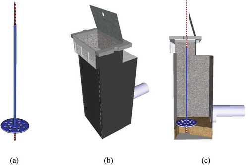
The volume of solids present is calculated by multiplying the bed thickness by the cross section of the gully pot. The solids accumulation rate is defined by the division of the change in solids volume by the number of days between consecutive measurements (in L/day):
In which S is the solids accumulation rate, A the horizontal cross section of the gully pot, di,g the ith measured depth in gully pot g, and t the measurement day.
Post et al. (Citation2016) showed that the sediment bed in most gully pots stabilised after a few months, which implies that S= 0. The current study is meant to determine the factors influencing the solids accumulation rate prior to the occurrence of gully pot blockages or the accumulation rate approaches zero. Therefore, in case of substantial sediment bed depths, all gully pots in a street were cleaned by the municipality on the authors’ request and a new measurement series was started, in this manner three measurement series for most streets were obtained during the monitoring period.
2.3. Parameters related to the accumulation rate
Post et al. (Citation2016) identified several parameters that influence the bed level in a gully pot, namely the connected area, road use, rainfall volume, and sand trap depth. In this study, parameters related to the build-up of solids on the street, the wash-off of these solids, and the retention of solids in the gully pot are added to the parameters mentioned above, to model the accumulation rate. These parameters are described in the next sections. The data used originate from readily available datasets from governmental organisations.
2.3.1. Parameters related to build-up
provides an overview of the parameters included in the model to schematise the build-up of solids on streets.
Table 1. Model parameters.
Table 2. Type of relations between the parameters and the accumulation rate in gully pots. Positive correlations are denoted with a plus sign and negative correlations with a minus sign.
Vegetation influences the solid loading on streets (e.g. Welker, Gelhardt, and Dierschke Citation2019; James and Shivalingaiah Citation1985), which subsequently influences the accumulation rate of solids in gully pots. Instead of monitoring the material loss of vegetation, a proxy is proposed to estimate the organic material potential. Both municipalities gave access to a dataset containing the tree types, locations, and heights. It is assumed that trees are dominant in the material loss by vegetation. Therefore, a vegetation factor is proposed and is defined per street, because leaves (and other organics) can easily spread over the street surface and end up in several gully pot catchments; and the trees were spread over the length of monitored streets.
The loss of material by a tree is assumed to be proportional to the size of the tree. The size is estimated by the cube of the tree height, which is known. This results in the following definition of the vegetation factor (in m2):
In which V is the vegetation factor, L is the length of the street, Hj is the height of tree j, and n is the total number of trees in the street. The vegetation factor is meant to represent the organic material potential. This potential varies over the year in reality (Welker, Gelhardt, and Dierschke Citation2019). Halverson, Gleason, and Heisler (Citation1985) distinguished four different phases for trees regarding the presence and absence of leaves, namely leaf abscission, leafless, leaf growth, and full capacity. These phases are combined in one categorical variable named tree phase. The start and end dates of the tree phases depend highly on climate and weather, and are based upon photos of the streets and trees made during the measurements. Only a few blossoming trees were present, which effect is therefore not separately analysed.
Traffic increases the solids loading on streets, due to vehicles losing material (e.g. Barrett et al. Citation1998; Kerri, Racin, and Howell Citation1985; Deletic, Ashley, and Rest Citation2000; Post et al. Citation2016; Simperler, Keckeis, and Ertl Citation2019). The pavement material and the pavement condition influence the availability and transport of solids over the street surface. This material also affects the infiltration capacity and, subsequently, the discharge into a gully pot.
The solids deposition in commercial areas is generally more than in residential areas (Sartor and Boyd Citation1972). This can be masked by street sweeping, which is often more frequently applied in commercial areas, and reduces the solids loading (Sutherland and Jelen Citation1997). Visual observation during the monitoring period made clear that the street surface close to shops contained more gross solids, which could be transported to gully pots, than residential areas.
2.3.2. Parameters related to wash-off
Build-up and wash-off models (see e.g. Sartor and Boyd Citation1972; Shaheen Citation1975; Pitt Citation1979; Egodawatta, Thomas, and Goonetilleke Citation2007; Muthusamy et al. Citation2018) include usually two or three processes to model the solids transport. Firstly, the accumulation of solids on the street, secondly the wash-off rate by rain, and sometimes the removal of solids by street sweeping. The second process is schematised in this section by the wash-off related parameters presented in .
The rainfall data used originate from the meteorological radar dataset of the Koninklijk Nederlands Meteorologisch Instituut (KNMI). This dataset contains 5-minute interval measurements on a 1 km2 grid. The 5-minute interval is used, because of the relatively small size of a gully pot catchment, which results in a short concentration time.
To represent rainfall intensity the maximum rainfall intensity is taken as a parameter, since it is the most important parameter for the wash-off in a rain event (Shivalingaiah and James Citation1984). The accumulation process is studied on a timescale of a few weeks (observation interval is 3–4 weeks), and is integrated over the time between two measurement days. This approach to a large extent filters out processes on a smaller timescale like the variation in rain intensity. Therefore, the wash-off in that period depends on the integral of the rainfall intensity as well, which is the rainfall volume (this dependency is also observed by Shaw, Stedinger, and Walter Citation2010).
The solids loading on streets is usually assumed to increase during dry periods (Sartor and Boyd Citation1972; Irish et al. Citation1995; Vaze and Chiew Citation2002; Chow, Yusop, and Abustan Citation2015; Morgan et al. Citation2017). Therefore, the initial loading and subsequently the transport of solids to the gully pot in a measurement interval depend on the length of the antecedent dry period.
2.3.3 Parameters related to retention
Butler and Karunaratne (Citation1995) studied the removal efficiency of gully pots in lab experiments and proposed an efficiency relation. Rietveld, Clemens, and Langeveld (Citation2020) showed that this equation is in most cases a valid (engineering) estimation of the initial efficiency.
In which ɳ is the efficiency, w is the settling velocity, Q is the discharge and A is the horizontal cross-sectional area of the gully pot. The equation contains two important concepts, namely the settling velocity and the surface loading. The settling velocity of a particle represents the gravitational force, while the surface loading represents the inertial force on a particle. The latter is defined as the discharge divided by the horizontal cross-sectional area. While the maximum rain intensity is assumed to be the main driver of solids wash-off, the maximum discharge is assumed to be the main driver of the gully pot hydraulics.
The settling velocity is not solely addressed in this study. This would involve a study of the variation in the solids characteristics at the monitored areas and over time. These processes are already represented by parameters related to the build-up (section 2.3.1). Studies as e.g. Bertrand-Krajewski, Briat, and Scrivener (Citation1993); Zafra, Temprano, and Tejero (Citation2008); Droppo et al. (Citation2006); Gelhardt, Huber, and Welker (Citation2017) addressed the solids characteristics.
Post et al. (Citation2016) showed that the sand trap depth is related to the accumulation of solids. Avila, Pitt, and Durrans (Citation2008) and Avila, Pitt, and Clark (Citation2011) observed that if the water depth above the sediment bed in the gully pot is sufficiently deep, the bed did not erode. Rietveld, Clemens, and Langeveld (Citation2020) concluded that the accumulation rate differed significantly from EquationEquation 3(3) when the sediment bed level increased, and eventually reduced to practically zero in conjunction with an equilibrium bed level and bed morphology. Butler and Clark (Citation1995) found that the equilibrium bed depth is close to the level of the outlet pipe. Therefore, the filling degree might be the parameter that influences the removal efficiency, rather than the bed depth itself.
The type of inlet influences the hydraulic conditions in the gully pot and could reduce the inflow of solids. The dataset contains gully pots with side inlets, top inlets, and combination inlets (Figure S3). However, considering combination inlets as a separate group could lead to wrong associations, since they are located in 1 street and their number in the dataset is limited (~4%). Since this kind of inlets is similar to side inlets from a hydraulic perspective, combination inlets are labelled as side inlets in the analysis. They have also been combined with the top inlets in the statistical analyses which did not significantly affect the results.
An overview of the parameters included in the model to schematise the retention of solids in gully pots is provided in .
2.4. Statistical modelling
A descriptive statistical model is required to identify the parameters which influence the accumulation rate of solids in gully pots. A regression tree and a linear mixed model are used to identify these parameters. Using two techniques could assist understanding the data structure and prevent method bias.
2.4.1. Regression tree
A Regression Tree (RT) is commonly used in data mining to explore the structure of datasets. A RT contains a rule at each node, which splits the dataset into two subsets. In this research, the criterion for the best split is defined as the split predictor that minimizes the p-value of chi-square tests of independence between each (pair of) explanatory variable(s) and the response variable. If all tests yield p-values larger than 0.05, splitting is stopped.
The procedure to obtain a single tree for the description of the data is based upon the procedure of De’ath and Fabricius (Citation2000) and consists of 6 steps:
Divide the data into n (in this study n = 5) random subsets of approximately equal size.
Cross-validate by dropping each subset in turn (test data) and build a tree using data from the remaining subsets (training data).
Predict the responses for the omitted subset, calculate the mean squared error for each subset and sum over all subsets.
Repeat steps (2)-(3) for a series of tree sizes.
Take the smallest tree (the pruned tree), such that the error is within one standard deviation of the minimum error of the cross-validation trees.
Repeat m times (in this study m = 50) steps (1)-(5) and select the most frequently occurring tree size from the distribution of selected tree sizes and subsequently a common tree.
2.4.2. Linear mixed model
Linear Mixed Models (LMMs) are suited for repeated measurements in different groups, which are in this case the individual gully pots. The model is described as:
In which Si,m,g is the ith observation of the solids accumulation rate in the mth measurement period in the gth gully pot, Xi,m,g,p the corresponding observation of explanatory variable p, bg is the random effect of gully pot g, and εi,m,g is the observation error. The random effect and observation error are described as:
The residuals of the accumulation rate in an individual gully pot could be related due to, for example, inaccurate values of the independent variables. The random effect compensates for these accumulation rate differences between gully pots. The observation error accounts for errors in all observations.
The model validation (shown in Appendix D) consists of 6 steps:
Take the training set, which was used to build the RT (as described in section 2.4.1) and build a LMM.
Remove observations with a Cook’s Distance larger than the 3 times the mean Cook’s Distance to avoid wrong associations due to influential outliers.Footnote2
Evaluate the homogeneity of the residuals.
Evaluate the independence of observations by analysing the correlation of residuals in time and space.
Remove step by step explanatory variables with p-values larger than 0.05.
Validate the LMM with the test set.
2.4.3. Sensitivity analysis
The accumulation rates found, as defined in EquationEquation 1(1) , are highly scattered due to two reasons. Firstly, the depth differences between two consecutive measurements (at a small measurement interval) are relatively small compared to the measurement uncertainty (~5 mm). Since the accumulation rate is the time derivative of the solid depth, the uncertainty in the accumulation rate is substantial. Secondly, processes with both short and long timescales, both on the street and in the gully pot determine the accumulation rate. These two reasons might influence the parameter identification by the models, which are based upon non-continuous measurements of the accumulation rate. Therefore, a sensitivity analysis is performed with a dataset with a different measurement interval.
The second dataset is composed of the same measurements, but every even measurement is leapfrogged, which effectively increases the measurement interval. This reduces the relative uncertainty in the accumulation rate, but reduces the size of the dataset and smoothens the processes influencing the accumulation rate. The latter can become a drawback, since time-dependent parameters (such as the rainfall volume and the tree phase) lose their meaning if the time interval becomes too large.
The reduced dataset is labelled as dataset 2. An overview of the range of the parameters in the two datasets is provided in Table S2.
3. Results
3.1. Explorative analysis
shows the measured sediment bed depth development in several gully pots. The depth generally increases over time, but sometimes decreases which could occur due to resuspension from the bed, and the process restarts after cleaning. EquationEquation 1(1) is used to calculate the accumulation rate from these measurements, which results in a dataset of 4173 data points with an average accumulation rate of +18 mL/day.
Figure 3. RT for dataset 1. The values at the nodes are the number of observations in the group and the mean accumulation rate of the group.
The Variance Inflation Factor (VIF) is used to assess the collinearity in the explanatory variables. Variables with a VIF larger than 10 are removed to avoid multicollinearity (as recommended by Montgomery, Peck, and Vining Citation2012). Initially, the VIF value associated with the filling degree exceeds 10 (shown in Table S3). The filling degree is closely related to the sand trap depth and the solid layer thickness. The physical process that is expected to be influenced by these parameters is the resuspension induced by the impinging jet of the inflowing water or the reduced settling due to increased local velocities (Rietveld, Clemens, and Langeveld Citation2020). The closer the sediment bed gets to the outlet pipe, the stronger these processes. To avoid overfitting and schematise this physical process, only the filling degree is selected as an explanatory variable, which makes all VIF values lower than 10.
3.2. Parameters related to the solids accumulation rate
The type of relation between the parameters and the accumulation rate of solids in gully pots (for dataset 1) is shown in . Parameters that correlate positively are denoted with a plus sign, whereas negative correlations with a minus sign. The β-values, standard errors, and p-values of the parameters used in the LMM are not provided here, but in Table S4. The RT with 9 terminal nodes is shown in .
Figure 2. Sediment bed depth development over time in 4 gully pots, which restarts after cleaning.
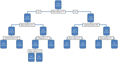
The RT contains less parameters than the LMM. The parameters used in the RT are also used in the LMM, except for the rainfall intensity which is negatively correlated with the accumulation rate in the RT. The LMM uses the discharge instead of the rainfall intensity (which are directly related) and shows a negative correlation with the accumulation rate.
Butler and Karunaratne (Citation1995) tested discharges between 0.5 L/s and 1.5 L/s and found an inversely proportional relation between the discharge and the removal efficiency. The same physical relation was expected in particular since the range of discharges in this study is even larger (between ~0.0029 and 16 L/s).
RT analysis allows investigating local relations within subgroups of the data. This reveals an interesting relation between the rainfall volume and the accumulation rate. The rainfall volume usually contributes positively, as this parameter represents the transport capacity of solids towards gully pots. However, it contributes negatively when it is combined with a high rainfall intensity. The rainfall intensity is related to the discharge to the gully pot, as stated above. An increased discharge results not only in less settling, but also in more resuspension from the sediment bed. This resuspension increases when the high rainfall intensity is combined with a large rainfall volume.
The removal efficiency, as described by EquationEquation 2(2) , contains not only the discharge, but also the cross-sectional area of the gully pot. However, this parameter is neither part of the LMM nor the RT. The range of cross-sectional areas (between ~0.045 and 0.16 m2) might be too small to detect significant differences and the hydraulic conditions could be described sufficiently by the water inflow (discharge or rainfall intensity) which have a wider spread. The parameters traffic intensity, pavement type, commercial area, and street sweeping don’t contribute significantly.
The antecedent dry period is negatively correlated with the accumulation rate in the LMM, which contradicts the results of Vaze and Chiew (Citation2002), who found that the solids loading on streets increases during dry days. However, other researchers (e.g. Ellis and Harrop Citation1984; Charbeneau and Barrett Citation1998; Kerri, Racin, and Howell Citation1985; Shaw, Stedinger, and Walter Citation2010) concluded that the length of the dry period prior to the storm event has only a weak relationship with the solids loading. Chow, Yusop, and Abustan (Citation2015) found that the maximum solids load on a street was reached in five dry days. Considering the fact that the measurement frequency was once in 3 to 4 weeks and that ~60% of the days during the monitoring were dry days, several dry and wet periods could occur in between two measurements. Therefore, the antecedent dry period is less relevant in this study.
The antecedent dry period also has the largest p-value of the parameters used in the LMM. This shows at least that a proper schematisation of the effect of dry periods on the solids loading on streets in a statistical model based on non-continuous measurements of the accumulation rate in gully pots is demanding. Therefore, a sensitivity analysis (which is provided in the next section) is important for this parameter.
The vegetation factor is positively correlated with the accumulation rate in the LMM. Welker, Gelhardt, and Dierschke (Citation2019) found that a relation between the presence of vegetation and the presence of solids on streets. These solids can be directed to gully pots via rain and wind. This process increases during the leaf abscission phase, which is therefore positively correlated with the accumulation rate. This confirms the conclusions of Chen et al. (Citation2017) who found that >50% of the gully pot blockages reported by citizens were registered in autumn.
The other parameters relating to the tree phases are negatively correlated with the accumulation rate when compared with the leaf abscission phase. The phases can also be mutually compared by their β-values. However, they do not differ significantly, considering the standard uncertainties.
The connected area is, similarly to the results of Post et al. (Citation2016), positively correlated with the accumulation rate in the LMM, since it is related to the amount of solids available for transport from the street. The LMM indicates that the geometry of the gully pot is important as well; gully pots with a top inlet show a higher accumulation rate than ones with a side inlet. From visual inspection, it appeared that grids of side inlets block more solids, which reduces the accumulation rate in those gully pots.
Finally, both models signify that the accumulation rate decreases as the sand trap gets filled, which is also observed in a lab study by Rietveld, Clemens, and Langeveld (Citation2020). This can be caused by two processes, namely the reduction of settling due to increased flow velocities and resuspension of solids from the sediment bed followed by transport to the drainage pipes.
3.3. Sensitivity analysis
A sensitivity analysis was performed to assess whether the selection of parameters (and their type of relation) is influenced by the uncertainty in the measurements (as discussed in section 2.4.3). Therefore, a second dataset is composed of accumulation rates over an increased time interval, by leapfrogging every even sediment depth measurement, resulting in a dataset of 3195 data points.
In general, the models (both the LMM and the RT) based upon dataset 2 identify the same type of relations as the models based upon dataset 1 (), confirming these findings. The main difference is the addition of extra parameters.
Figure S7 shows the RT for the dataset with an increased time interval. The tree consists of 17 terminal nodes, while the one based upon the original dataset consists of 9 terminal nodes, this implies that the data patterns also more discernible due to the reduced uncertainty.
Moreover, the performance (although still poor) of the models based upon dataset 2 improves significantly compared with the ones based upon dataset 1 (Table S5). The R2 values indicate that the RTs fit the measurements better than the LMMs. The RT for dataset 2 explains 29% of the variance in the training data and 17% in the test data.
The LMMs based upon dataset 1 and 2 contain the same parameters, except for the pavement type. This parameter has a p-value close to 0.05 and its impact is, therefore, less clear than other parameters. The only remaining difference is the type of relation of the antecedent dry period. This parameter is negatively correlated with the accumulation rate in dataset 1, while it is positively correlated in dataset 2. A positive correlation is expected, since solids loading on streets increases during dry days (Vaze and Chiew Citation2002). The RT based upon dataset 2 contains this positive relation as well.
The impact of street sweeping on the accumulation rate is discussed in literature and is generally found to be more effective for large debris than small particles (e.g. Pitt et al. Citation2005; Walker and Wong Citation1999; Amato et al. Citation2010). Sutherland and Jelen (Citation1997) concluded that outdated street sweeping technologies could not pick up the finer solids and increased solids loadings to gully pots by loosening immobile solids. It was concluded that sweeping technology improved meanwhile and became efficient in reducing solids loadings. However, Walker and Wong (Citation1999) concluded that the benefits of increasing the frequency of street sweeping, beyond what is required to meet street aesthetic criterion, is expected to be small in relation to water quality improvements. In this study, the sweeping frequency is found to correlate positively with the accumulation in dataset 2. Figure S7 shows that sweeping is the second decision parameter. It splits observations from 5 streets, in subgroups representing 2 and 3 streets. Research in more streets is needed to verify that this is not coincidental and actually represents a missing parameter. Another verification method is to change the street sweeping frequency in a street that is monitored over time.
The importance of the connected area and the parameters relating to the tree phases is emphasised by the fact that they are part of both LMMs and for the RT based on dataset 2. The split in the categorical parameter tree phase in the RT is made between at one side the leaf abscission and leaf growth phase and at the other side the leafless and the full capacity phase. The LMMs show that the leaf abscission phase is the main contributor to the accumulation rate.
Although the LMMs show a negative relation between the discharge and the accumulation rate, the RT in Figure S7 shows a positive relation. The significance of this relation is judged to be low, however: the parameter only appears in the lowest ranks of the tree, and, moreover, the split is defined such that only a few observations end up in one of the subgroups.
4. Discussion
The parameters selected by the LLMs and the RTs as being the most important in terms of describing the experimental data provide hints to identify the dominant processes in the solids accumulation rate in a batch of gully pots. However, since the model results show small R2 values, the measured solids accumulation rate in a single gully pot cannot be successfully reproduced by these models.
A common characteristic of reported projects looking into the build-up and wash-off of solids from urban surfaces over the past decades (Sartor and Boyd Citation1972; Pitt Citation1979; Pratt and Adams Citation1984; Ellis and Harrop Citation1984; Pitt et al. Citation2005) is the fact that no generic conclusions have been drawn on the quantifiability of the solids loading from runoff, then site-specific statistical relations between solids loading and, for instance, rainfall parameters, presence of trees etc. It is a well-known fact that non-linear systems having feedback processes may initiate unpredictable dynamic behaviour, also referred to as chaotic behaviour (Genesio and Tesi Citation1991). In literature, some indications for such behaviour for wash-off related processes are found.
Post et al. (Citation2016) monitored the sediment bed development of ~300 gully pots and found that ~5% got clogged due to a growing bed after ~15 months, while the sediment bed of the remaining ~95% reached an equilibrium in a few months. A clear difference between these two groups of gully pots causing this difference could not be determined.
Naves et al. (Citation2020) performed lab experiments on the wash-off from an artificial street surface and modelled this with a physically-based model. They found that despite the accurate definition of the (initial) conditions (such as the solids load on the street and the rainfall), a wide range of model (calibration) parameters was possible.
Vaze and Chiew (Citation2002) measured the solids load in three zones of a 300 m long street over a period of 36 days on an almost dayly basis. The results showed that the correlations in the solids load (collected from surfaces of 0.5 m2) between the three zones over the 36 days period are relatively low, which indicated that the spatial variability of the load is quite high. Liu, Goonetilleke, and Egodawatta (Citation2012) found that the variability of some build-up parameters within the same land use is higher than the variability between land uses.
Since the statistical models in the current study are applied to monitoring data from strongly varying spatial and temporal environments, a small R2 value on the level of an individual gully pot could be expected. Nevertheless, patterns in the accumulation rate of solids in gully pots can and are recognised by monitoring a batch of gully pots. The limited predictability in this study and related problems in other studies may be due to inherent randomness in the processes (e.g. rain-induced uncertainty), or even non-linear feedbacks in these processes causing inherent unpredictability (chaos). Further research may assess whether the latter is the case, and if so what would be the prediction horizon. This would require more frequent and more precise observations of the sediment bed development, which proved to be impossible with the method used in this study, since the observation uncertainty relative to the bed growth is too large.
If the solids accumulation rate is not chaotic or is predictable for a substantial period, such a study could be used to assess whether the reduction in uncertainty in both the bed depth measurements and the explanatory variables could improve the accuracy of the models significantly, as the model parameters are not fully independent, represent short- and long-term processes, and describe processes on the street and in the gully pot, reducing the predictability of statistical models based upon non-continuous measurements.
To reduce the uncertainty in the accumulation rate, a non-invasive measurement technique is required which measures at a high precision (a discussion on sewer inspection techniques can be found in Tscheikner-Gratl et al. Citation2019). Optical techniques are not likely to be effective due to the different material phases and the dirty environment. Lepot et al. (Citation2017) showed that sonar (which is a non-invasive technique) provides relatively small uncertainties in locating the surface of sediment layers in a sewer pipe.
The biggest advantage could be gained if sonar would be installed in the gully pot for continuous measurements to analyse the impact of individual storm events. This is substantially more expensive than the current approach (and requires some engineering for installation), especially since a considerable amount of gully pots (and therefore sonars) is required for reliable analyses.
Another measurement technique to determine the sediment level, could be transferring radio waves (Moghadas, Mirzavand, and Mousav Citation2019) or current from one side to the other of the height of the gully pot. However, these techniques have not been applied in drainage systems yet, to the authors’ knowledge.
The vegetation factor, rainfall volume, rainfall intensity, and filling degree are the most important parameters in the RTs. The LMMs add the connected area, tree phase, discharge, and inlet type to these parameters. The most important uncertainties are found in the rainfall intensity (and consequently the discharge) and the vegetation factor. These uncertainties could be reduced by using other measurement techniques.
The discharge could be measured with discharge meters in the gully pot outlet pipes, which requires a large investment in discharge meters. These measurements can also be used to correct the connected area by comparing the discharge in adjacent gully pots.
The vegetation factor is a proxy for the amount of organic material from trees, but does not include the type of trees, other types of vegetation in the public area, or vegetation in nearby private areas. Including these parameters would make the vegetation factor more representative, but the introduction of more parameters requires also a larger dataset.
Another approach is to define a parameter that directly represents the organic material from trees present on streets. Cameras could be installed and some recognition software has to be developed. This would make the parameters that represent the tree phase redundant. Nevertheless, both approaches require a major effort.
5. Conclusions
The objective of the study was to assess to what extent the accumulation rate is influenced by physical parameters linked to the build-up of solids in a catchment, the wash-off of these solids from this catchment, and the retention of solids in the gully pot. Several parameters are identified with Linear Mixed Models (LMMs) and Regression Trees (RTs). The performance of RTs in this study is better than the LMMs, most likely due to their capability to describe different relationships between explanatory and response variables in different parts of the measurement space, which is necessary to identify the impact of parameters which are related to the accumulation rate in both a positive and negative way, such as the rainfall volume. This parameter usually contributes positively, since it increases the transport capacity, but combined with a high rainfall intensity it contributes negatively, due to increased erosion of the sediment bed.
The parameters vegetation factor, rainfall volume, and filling degree appeared in all models. Therefore, it is concluded that these are the main drivers of the accumulation rate of solids in gully pots. This implies that none of the three processes (build-up of solids in a catchment, the wash-off of these solids from this catchment, and the retention of solids in the gully pot) dominates the accumulation rate.
The sensitivity analysis shows that the parameter identification by the RT is more sensitive than the LMM for the relatively high uncertainties in dataset 1 compared to dataset 2. The sensitivity analysis indicates that the accumulation rate is also dependent on other factors (i.e. connected area, tree phase, rainfall intensity, discharge, and inlet type).
The R2 values of these models are modest, indicating that the solids accumulation rate in a single gully pot cannot be predicted by the models, which raises questions to what extend the models are generalisable to other spatial and temporal environments, and even (combined with literature) whether the solids accumulation would be inherently chaotic. These questions may be addressed in further research, since it affects the required research methodology. Firstly, a thorough analysis should be made of the dynamics of the individual processes influencing the accumulation rate, such as rainfall, build-up, erosion, settling etc. Secondly, it should be analysed how the potential chaotic behaviour of these processes influence the dynamics of the solids accumulation.
If the solids accumulation process is not chaotic, it could be studied whether the reduction in uncertainty in both the bed depth measurements and the explanatory variables could improve the accuracy of the models significantly. Such a study could involve more frequent or even (semi-) continuous monitoring of the sediment bed depth and more precise measurements of the explanatory variables. The parameters ‘vegetation factor ‘and the ‘discharge’ (or rainfall intensity) are the most important parameters in this respect.
Supplemental Material
Download PDF (1.1 MB)Acknowledgements
The authors thank the municipalities of Rotterdam and Den Haag for providing the measurement locations and practical help. They thank Nadia Mobron, André Vallendar, and Cédric Zigault who have been working on this project as part of their study curriculum.
Disclosure statement
No potential conflict of interest was reported by the author(s).
Supplementary material
Supplemental data for this article can be accessed here
Additional information
Funding
Notes
1. The measured depth is dependent on the gas fraction and the compressibility of the bed, by compressing the sediment before the depth measurement, which improves the reproducibility of the measurement.
2. Whenever possible the cause of the outliers was identified using the logbooks or other circumstantial evidence that exceptional situations occurred.
References
- Amato, F., X. Querol, C. Johansson, C. Nagl, and A. Alastuey. 2010. “A Review on the Effectiveness of Street Sweeping, Washing and Dust Suppressants as Urban PM Control Methods.” Science of the Total Environment 408 (16): 3070–3084. doi:10.1016/j.scitotenv.2010.04.025.
- Ashley, R. M., A. Fraser, R. Burrows, and J. Blanksby. 2000. “The Management of Sediment in Combined Sewers.” Urban Water 2 (4): 263–275. doi:10.1016/S1462-0758(01)00010-3.
- Ashley, R. M., D. J. Wotherspoon, M. J. Goodison, and I. Mcgregor. 1992. “The Deposition and Erosion of Sediments in Sewers.” Water Science Technology 26 (5–6): 1283–1293. doi:10.2166/wst.1992.0571.
- Avila, H., R. Pitt, and S. E. Clark. 2011. “Development of Effluent Concentration Models for Sediment Scoured from Catchbasin Sumps.” Journal of Irrigation and Drainage Engineering 137 (3): 114–120. doi:10.1061/(ASCE)IR.1943-4774.0000183.
- Avila, H., R. Pitt, and S. R. Durrans. 2008. “Factors Affecting Scour of Previously Captured Sediment from Stormwater Catchbasin Sumps.” Journal of Water Management Modeling. doi:10.14796/JWMM.R228-13.
- Barrett, M. E., J. L. B. Irish Jr, J. F. Malina Jr, and R. J. Charbeneau. 1998. “Characterization of Highway Runoff in Austin, Texas, Area.” Journal of Environmental Engineering 124 (2): 131–137. doi:org//10.1061/(ASCE)0733-9372(1998)124:2(131).
- Bertrand-Krajewski, J. L., P. Briat, and O. Scrivener. 1993. ““Sewer Sediment Production and Transport Modelling: A Literature Review.” Journal of Hydraulic Research 31 (4): 435–460. doi:10.1080/00221689309498869.
- Bolognesi, A., A. Casadio, A. Ciccarello, M. Maglionico, and S. Arina 2008. “Experimental Study of Roadside Gully Pots Efficiency in Trapping Solids Washed off during Rainfall Events.” In Proceedings of the 11th International Conference on Urban Drainage. Edinburgh, Scotland.
- Butler, D., and P. Clark. 1995. Sediment Management in Urban Drainage Catchments. London: Construction Industry Research & Information Association.
- Butler, D., and S. H. P. G. Karunaratne. 1995. “The Suspended Solids Trap Efficiency of the Roadside Gully Pot.” Water Research 29 (2): 719–729. doi:10.1016/0043-1354(94)00149-2.
- Charbeneau, R. J., and M. E. Barrett. 1998. “Evaluation of Methods for Estimating Stormwater Pollutant Loads.” Water Environment Research 70 (7): 1295–1302. doi:10.2175/106143098X123679.
- Chen, Y., P. Cowling, F. Polack, S. Remde, and P. Mourdjis. 2017. “Dynamic Optimisation of Preventative and Corrective Maintenance Schedules for a Large Scale Urban Drainage System.” European Journal of Operational Research 257 (2): 494–510. doi:10.1016/j.ejor.2016.07.027.
- Chow, M. F., Z. Yusop, and I. Abustan. 2015. “Relationship between Sediment Build-up Characteristics and Antecedent Dry Days on Different Urban Road Surfaces in Malaysia.” Urban Water Journal 12 (3): 240–247. doi:10.1080/1573062X.2013.839718.
- Crabtree, R. W. 1989. “Sediment in Sewers.” Water and Environment Journal 3 (6): 569–578. doi:10.1111/j.1747-6593.1989.tb01437.x.
- De Man, H., H. H. J. L. Van den Berg, E. J. T. M. Leenen, J. F. Schijven, F. M. Schets, J. C. Van der Vliet, F. Van Knapen, and A. M. De Roda Husman. 2014. “Quantitative Assessment of Infection Risk from Exposure to Waterborne Pathogens in Urban Floodwater.” Water Research 48: 90–99. doi:10.1016/j.watres.2013.09.022.
- De’ath, G., and K. E. Fabricius. 2000. “Classification and Regression Trees: A Powerful yet Simple Technique for Ecological Data Analysis.” Ecology 81 (11): 3178–3192. doi:10.1890/0012-9658(2000)081[3178:CARTAP]2.0.CO;2.
- Deletic, A., and D. W. Orr. 2005. ““Pollution Buildup on Road Surfaces.” Journal of Environmental Engineering 131 (1): 49–59. doi:org//10.1061/(ASCE)0733-9372(2005)131:1(49).
- Deletic, A., R. M. Ashley, and D. Rest. 2000. “Modelling Input of Fine Granular Sediment into Drainage Systems via Gully Pots.” Water Research 34 (15): 3836–3844. doi:10.1016/S0043-1354(00)00133-0.
- Droppo, I. G., K. N. C. K. J. Irvine, E. Carrigan, S. Mayo, C. Jaskot, and B. Trapp. 2006. “26 Understanding the Distribution, Structure and Behaviour of Urban Sediments and Associated Metals toward Improving Water Management Strategies.” In Soil Erosion and Sediment Redistribution in River Catchments: Measurement, Modelling and Management. Wallingford, UK: CABI.
- Egodawatta, P., E. Thomas, and A. Goonetilleke. 2007. “Mathematical Interpretation of Pollutant Wash-off from Urban Road Surfaces Using Simulated Rainfall.” Water Research 41 (13): 3025–3031. doi:10.1016/j.watres.2007.03.037.
- Ellis, J. B., B. Chocat, J. Fujita, J. Marsalek, and W. Rauch. 2004. Urban Drainage. London: IWA Publishing.
- Ellis, J. B., and D. O. Harrop. 1984. “Variations in Solids Loadings to Roadside Gully Pots.” Science of the Total Environment 33 (1–4): 203–211. doi:10.1016/0048-9697(84)90394-2.
- Gelhardt, L., M. Huber, and A. Welker. 2017. “Development of a Laboratory Method for the Comparison of Settling Processes of Road-Deposited Sediments with Artificial Test Material.” Water, Air, and Soil Pollution 228 (12): 467. doi:10.1007/s11270-017-3650-8.
- Genesio, R., and A. Tesi. 1991. “Chaos Prediction in Nonlinear Feedback Systems.” IEE Proceeding D-control Theory and Apllications 138 (4): 313–320. doi:10.1049/ip-d.1991.0042.
- Halverson, H. G., S. B. Gleason, and G. M. Heisler. 1985. “Leaf Duration and the Sequence of Leaf Development and Abscission in Northeastern Urban Hardwood Trees.” Urban Ecology 9 (3–4): 323–335. doi:10.1016/0304-4009(86)90007-0.
- Herngren, L. F. 2005. Build-up and Wash-off Process Kinetics of PAHs and Heavy Metals on Paved Surfaces Using Simulated Rainfall. Brisbane: Queensland University of Technology.
- Het Samenwerkingsorgaan Holland Rijnland. 2015. Actualisatie En Harmonisatie Van Het Verkeersmodel Holland Rijnland [Update and Harmosation of the Holland Rijnland Traffic Model]. Leiden: Holland Rijnland.
- Irish, L. B., Jr, W. G. Lesso, M. E. Barrett, J. F. Malina Jr, R. J. Charbeneau, and G. H. Ward. 1995. An Evaluation of the Factors Affecting the Quality of Highway Runoff in the Austin, Texas Area. Austin: Center for Research in Water Resources, The University of Texas at Austin.
- James, W., and B. Shivalingaiah. 1985. “Storm Water Pollution Modelling: Buildup of Dust and Dirt on Surfaces Subject to Runoff.” Canadian Journal of Civil Engineering 12 (4): 906–915. doi:org//10.1139/l85-103.
- Jenson, S. K., and J. O. Domingue. 1988. “Extracting Topographic Structure from Digital Elevation Data for Geographic Information System Analysis.” Photogrammetric Engineering and Remote Sensing 54 (11): 1593–1600.
- Kerri, K. D., J. A. Racin, and R. B. Howell. 1985. “Forecasting Pollutant Loads from Highway Runoff.” Transportation Research Record 1017: 39–46.
- Langeveld, J. G., E. Liefting, and R. Schilperoort. 2016. Regenwaterproject Almere [Storm Water Project Almere]. Amersfoort: Stichting RIONED en STOWA.
- Lepot, M., T. Pouzol, X. A. Borruel, D. Suner, and J.-L. Bertrand-Krajewski. 2017. “Measurement of Sewer Sediments with Acoustic Technology: From Laboratory to Field Experiments.” Urban Water Journal 14 (4): 369–377. doi:10.1080/1573062X.2016.1148181.
- Liu, A., A. Goonetilleke, and P. Egodawatta. 2012. “Inherent Errors in Pollutant Build-up Estimation in considering Urban Land Use as a Lumped Parameter.” Journal of Environmental Quality 41 (5): 1690–1694. doi:10.2134/jeq2011.0419.
- Moghadas, H., R. Mirzavand, and P. Mousavi. 2019. “Early Detection of Flood in Urban Catch Basins Using Radio Frequency Slot Line Array.” Measurement 134: 515–518. doi:10.1016/j.measurement.2018.10.102
- Montgomery, D. C., E. A. Peck, and G. G. Vining. 2012. Introduction to Linear Regression Analysis. New York: John Wiley & Sons.
- Morgan, D., P. Johnston, K. Osei, and L. Gill. 2017. “Sediment Build-up on Roads and Footpaths of a Residential Area.” Urban Water Journal 14 (4): 378–385. doi:10.1080/1573062X.2016.1148182.
- Muthusamy, M., S. Tait, A. Schellart, M. N. A. Beg, R. F. Carvalho, and J. L. de Lima. 2018. “Improving Understanding of the Underlying Physical Process of Sediment Wash-off from Urban Road Surfaces.” Journal of Hydrology 557: 426–433. doi:10.1016/j.jhydrol.2017.11.047.
- Naves, J., J. Rieckermann, L. Cea, J. Puertas, and J. Anta. 2020. “Global and Local Sensitivity Analysis to Improve the Understanding of Physically-based Urban Wash-off Models from High-resolution Laboratory Experiments.” Science of the Total Environment 709. doi:10.1016/j.scitotenv.2019.136152.
- Novotny, V., H. M. Sung, R. Bannerman, and K. Baum. 1985. “Estimating Nonpoint Pollution from Small Urban Watersheds.” Journal of Water Pollution Control Federation 57 (4): 339–348.
- Pitt, R. 1979. Demonstration of NonPoint Pollution Abatement through Improved Street Cleaning Practices. Washington DC: U.S. EPA.
- Pitt, R., D. Williamson, J. Voorhees, and S. Clark. 2005. “Review of Historical Street Dust and Dirt Accumulation and Washoff Data.” Journal of Water Management Modeling. doi:10.14796/JWMM.R223-12.
- Post, J. A. B., I. W. M. Pothof, J. Dirksen, E. J. Baars, J. G. Langeveld, and F. H. L. R. Clemens. 2016. “Monitoring and Statistical Modelling of Sedimentation in Gully Pots.” Water Research 88: 245–256. doi:10.1016/j.watres.2015.10.021.
- Pratt, C. J., and J. R. W. Adams. 1984. “Sediment Supply and Transmission via Roadside Gully Pots.” Science of the Total Environment 33 (1–4): 213–224. doi:10.1016/0048-9697(84)90395-4.
- Rietveld, M. W. J., F. H. L. R. Clemens, and J. G. Langeveld. 2020. “Solids Dynamics in Gully Pots.” Urban Water Journal.
- Sartor, J. D., and G. B. Boyd. 1972. Water Pollution Aspects of Street Surface Contaminants. Washington DC: U.S.EPA.
- Shaheen, D. G. 1975. Contributions of Urban Roadway Usage to Water Pollution. Washington DC: U.S.EPA.
- Shaw, S. B., J. R. Stedinger, and M. T. Walter. 2010. “Evaluating Urban Pollutant Buildup/wash-off Models Using a Madison, Wisconsin Catchment.” Journal of Environmental Engineering 136 (2): 194–203. doi:10.1061/(ASCE)EE.1943-7870.0000142.
- Shivalingaiah, B., and W. James 1984. “Algorithms for Buildup, Washoff, and Routing Pollutants in Urban Runoff.” In Proceedings of the Third International Conference on Urban Storm Drainage. Göteborg, Sweden.
- Simperler, L., K. Keckeis, and T. Ertl 2019. “Using a Solids Mass Balance Model for Impact Estimation of Stormwater Management Measures on Sewer Operation.” In Proceedings of the Ninth International Conference on Sewer Processes & Networks. Aalborg, Denmark.
- Sutherland, R. C., and S. L. Jelen. 1997. “Contrary to Conventional Wisdom, Street Sweeping Can Be an Effective BMP.” In Advances in Modeling the Management of Stormwater Impacts. Guelph, Canada: CHI.
- Ten Veldhuis, J. A. E., and F. H. L. R. Clemens. 2011. “The Efficiency of Asset Management Strategies to Reduce Urban Flood Risk.” Water Science & Technology 64 (6): 1317–1324. doi:10.2166/wst.2011.715.
- Tscheikner-Gratl, F., N. Caradot, F. Cherqui, J. P. Leitão, M. Ahmadi, J. G. Langeveld, Y. Le Gat, et al. 2019. “Sewer Asset Management – State of the Art and Research Needs.” Urban Water Journal 16 (9): 662–675. doi:10.1080/1573062X.2020.1713382.
- Van Bijnen, M., H. Korving, J. G. Langeveld, and F. H. L. R. Clemens. 2018. “Quantitative Impact Assessment of Sewer Condition on Health Risk.” Water 10 (3): 245–257. doi:10.3390/w10030245.
- Van der Zon, N. 2013. Kwaliteitsdocument AHN2 [Quality Document AHN2]. Amersfoort: Rijkswaterstaat & Waterschappen.
- Vaze, J., and S. Chiew. 2002. “Experimental Study of Pollutant Accumulation on an Urban Road Surface.” Urban Water 4 (4): 379–389. doi:10.1016/S1462-0758(02)00027-4.
- Walker, T. A., and T. H. F. Wong. 1999. Effectiveness of Street Sweeping for Stormwater Pollution Control. Melbourne: Cooperative Research Centre for Catchment Hydrology.
- Welker, A., L. Gelhardt, and M. Dierschke 2019. “Vegetation and Temporal Variability of Particle Size Distribution (PSD) and Organic Matter of Urban Road Deposited Sediments in Frankfurt Am Main.” In Proceedings of Novatech 2019. Lyon, France.
- Zafra, C. A., J. Temprano, and I. Tejero. 2008. “Particle Size Distribution of Accumulated Sediments on an Urban Road in Rainy Weather.” Environmental Technology 29 (5): 571–582. doi:10.1080/09593330801983532.