A model-based estimate of the groundwater budget and associated uncertainties in Bengaluru, India

ABSTRACT

Understanding the water metabolism of developing country cities is challenging because of insufficient knowledge of how social, infrastructural and hydrological dimensions are coupled. Using Bengaluru City in India, we demonstrate how fine-resolution data can inform model-based estimates of urban groundwater budgets. Groundwater levels were measured at 154 locations in 2016 and used to estimate model parameters and uncertainty. Total water use was estimated at 1470 million litres per day (MLD). Groundwater pumping meets the majority of this use (827 MLD), followed by utility water supply (643 MLD). Total recharge was estimated at 973 MLD. Natural recharge is a much smaller portion (183 MLD) compared to anthropogenic recharge from leaking water supply and wastewater systems (791 MLD). The city experienced a net negative groundwater balance (40 MLD). Natural recharge and total water use estimates showed lower uncertainty. Spatial variation in these fluxes is described and related to secondary information.

KEYWORDS:

• Groundwater
• urban
• anthropogenic
• modelling
• Bengaluru
• metabolism

Introduction

Cities are tightly coupled socio-ecological systems (Schandl and Capon 2012) sustained by metabolic flows of various resources (Wolman 1965; Kennedy, Cuddihy, and Engel-Yan 2007). Water is the largest metabolic flow and urbanization affects the water cycle in both quantity and quality (Vázquez-Suñé, Sánchez-Vila, and Carrera 2005; Decker et al. 2000). Several aspects of urban hydrology distinguish it from that of natural systems. Large amounts of water are imported, distributed and collected again in sewers and septic tanks. Leaking water supply lines, sewer mains and septic tanks comprise anthropogenic elements of groundwater recharge, that add to natural recharge from precipitation. Anthropogenic recharge was found to constitute 20% to 50% of total recharge in some cases (Lerner 2002). On the negative side of the groundwater budget, pumping is the anthropogenic element which can dominate the urban groundwater balance.

Examples from some major cities illustrate the anthropogenic effects on water balances. In Seoul, Korea, groundwater pumping and leaking water mains were dominant components of the city’s groundwater budget (Kim, Lee, and Sung 2001). While the effect on groundwater level was not substantial because leakages made up for extraction, water quality was impaired because of recharge from leaking sewers and septic tanks. The dynamic nature of socio-hydrological coupling means that policies surrounding land and water management can have long-lasting and surprising consequences. In Tokyo, in response to groundwater over-extraction in the 1950s and 1960s, groundwater pumping was replaced with imported surface water supply. Groundwater levels recovered over ensuing decades; however, during this time, a massive underground rail infrastructure was put in place. Groundwater levels are now endangering this underground infrastructure (Hayashi et al. 2009). Similar examples can be found in several other cities around the world including Milan, Italy (Gattinoni and Scesi 2017) and in the U.K. (Hurst and Wilkinson 1986; Brassington and Rushton 1987; Brassington 1990).

Lerner (2002) and Vázquez-Suñé, Sánchez-Vila, and Carrera (2005), in reviewing the particular challenges of understanding urban groundwater budgets, included the following: (i) the90 complexity of sources and pathways of recharge; (ii) the need for large amounts of data, from various sources and (iii) prevalence of large uncertainties and data gaps. Additionally, estimating groundwater budgets is especially difficult in cities of the developing world given the many water sources and modes of supply that people rely on and the wide variation in supply across different parts of these cities (Foster, Lawrence, and Morris 1998; Jaglin 2014). India’s urban water supply scenario is illustrative of this. On the demand side, since no city receives 24 × 7 water supply, consumers obtain water from multiple sources, including utility piped supply, tankers, private groundwater wells, bottled water and untreated water bodies (Srinivasan, Gorelick, and Goulder 2010; Misra and Goldar 2008). As a result, ‘no city municipality knows what the real water demand is in the spaces they govern’ (Narain and Pandey 2012).

Although almost all of the above mentioned alternate sources rely on groundwater, the existing groundwater monitoring network is too coarse to understand the groundwater status of urban centres. Groundwater resources assessments in the country are typically conducted at river basin or state-wide scale, relying on a combination of GIS, remote sensing, and a national groundwater monitoring framework that samples at a coarse density. For instance, in Karnataka state, the monitoring well density is 1 per 100 km² and measurements are taken 4 times in a year during January, May, August and November (Central Groundwater Board 2016). Urban landscapes usually cover areas in the range of tens to few hundreds of km² and are highly heterogeneous. Therefore, these require a much denser monitoring network than what currently exists. Both the demand and supply sides of the (ground)water budget are ill-informed in India.

Consequently, the socio-hydrology of Indian cities remains poorly understood, especially from a quantitative and spatially disaggregated standpoint (Mehta et al. 2013). This poses a serious challenge given India’s rapid urbanization (Planning Commission 2013), lack of adequate water supply, wastewater treatment and sanitation (Narain and Pandey 2012), and the sheer fact of it being the largest user of freshwater and groundwater in the world (Gilbert 2012). As of 2015, there were only two quantitative socio-hydrological assessments: hydroeconomic modelling of Chennai and its water supply system (Srinivasan, Gorelick, and Goulder 2010) and the groundwater study of the small town of Mulbagal (Sekhar et al. 2013).

In order to address these gaps, we began monitoring groundwater levels in 154 wells across Bengaluru city at monthly frequency from December 2015, with the overall objectives of understanding the groundwater budget and spatio-temporal behaviour with the help of data and models. A first set of results was produced in 2017 (Sekhar et al. 2017), describing the spatio-temporal behaviour of groundwater levels measured in 2016. A simple, vertical, Water Table Fluctuation (WTF) method was used to estimate groundwater storage change, natural (rainfall) recharge and net groundwater outflow. In this paper, we use a more refined and elaborate model to disaggregate the natural and anthropogenic components of net outflow, while also incorporating other infrastructural and socio-economic data. The Generalized Likelihood Uncertainty Estimation (GLUE) approach (Beven and Binley 1992) was used to compute uncertainties in various components of the groundwater balance. Our objective was to develop and spatially disaggregate the urban groundwater budget for Bengaluru, with a specific interest in estimating draft (pumping) and recharge.

Materials and methods

Study area

Climate and physiography

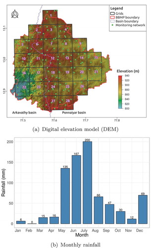
The Greater Bangalore Metropolitan Corporation called Bruhat Bengaluru Mahanagara Palike (BBMP) has an area of approximately 741 km² and lies between 12°48ʹ-13°9ʹN latitude and 77°27ʹ-77°47ʹ longitude. The city core is above mean sea level, on a divide with a roughly North-South axis, with the Arkavathi river drainage westward, and the Ponnaiyar drainage to the East (Figure 1). The climate is classified as ’topical savannah (Aw)’ in the Köppen–Geiger classification system (Beck et al. 2018), with a long-term mean annual rainfall of 820 mm (Sekhar et al. 2017). Monthly rainfall during the study period (January 2016–December 2016) is shown in Figure 1. 764 mm rainfall occurred in 2016, of which 75% was received from May–August. The Arkavati river basin has NNE-SSW and ENE-WSW lineaments, while the Ponnaiyar drainage is along the NW-SE and WSW-ENE fractures. The city is underlain by Precambrian granite and gneiss, weathered to a maximum depth of 60 m, covered by red loamy and gravelly soils. The aquifer system in the larger Bengaluru urban district is a combination of this shallow weathered zone and the underlying hard rock system (CGWB 2011; Sekhar and Kumar 2009). Hard-rock aquifers of this kind are characterized by low hydraulic conductivity (10–65 m²/d) and specific yield (0.005–0.01) and high lateral heterogeneity. Bore-well yields are typically very low, from 0.8 to 5 litre/s. A typical weathering profile is presented in Maréchal, Dewandel, and Subrahmanyam (2004). The saprolite or regolith is a clay-rich material derived from prolonged in situ decomposition of bedrock and is few tens of meters thick. The saprolite can reach a quite high porosity, depending on lithology of parent rock, and generally has low conductivity.

Figure 1. DEM and monthly rainfall during the study period (January – December, 2016)

(a) Digital elevation model (DEM); (b) Monthly rainfall.

Recharge to the system will be through the shallow weathered zone, and from there some water will drain into the deeper fractured rock aquifer. Given this difference in character, they may appear to be independent aquifers, but in the longer term and on a broad scale they will be interconnected. The saprolite, when saturated, provides the capacitive role while the fissured layer provides the transmissivity role of the global composite aquifer. Several studies that are at a non-local, larger scale, have used simplifying assumptions regarding transmissivity and specific yield that can be interpreted as effective parameters of this global composite aquifer (Sekhar et al. 2017, 2013; Sekhar and Kumar 2009). More details on the hydrogeological conceptual model are provided in supplementary material S2.

Population growth and status of water infrastructure

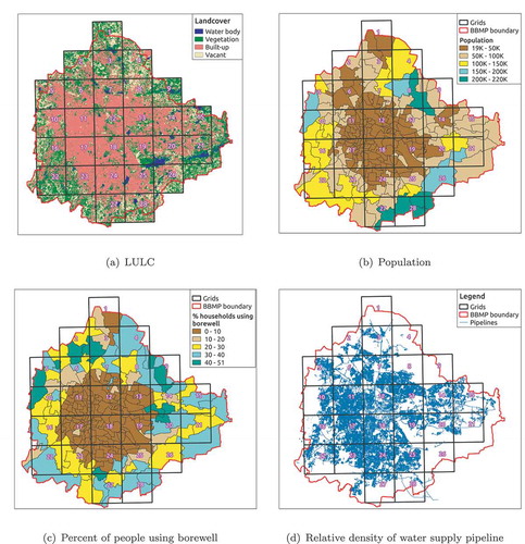
Bengaluru, with its origins in the 12^th century, has undergone a rapid transformation in recent decades that is continuing today. Figure 2 illustrates some of the key characteristics of the city. Bengaluru is the capital of Karnataka state and is one of the fastest growing urban agglomeration for 2001–2010 (Census 2011). It grew from 1.65 million people in 1971 to 8.5 million people in 2011, during which time its built-up area increased from 20% to approximately 70% of its corresponding municipal boundaries (Mehta et al. 2013). Population growth between 2001 and 2011 has been especially rapid with some city wards growing 150%-300%. The public water supply from the utility – called the Bengaluru Water Supply and Sewerage Board (BWSSB) – is largely dependent on imported water from the Cauvery river which is approximately 100 km away, against a total head of about 500 m.

Figure 2. Spatial distribution of relevant variables in Bengaluru. (a) Land Use-Land Cover (LULC) is based on Balakrishnan (2016), (b) population, (c) percentage of households using borewells and (d) relative density of water supply pipeline

(a) LULC; (b) Population; (c) Percent of people using borewell; (d) Relative density of water supply pipeline.

While BWSSB supply has also grown in several phases, it has not been able to keep up (Mehta et al. 2014). With the fastest population growth occurring in outer areas, a negative correlation between population growth and per capita water supplied has been observed, testifying to the challenges in keeping up with the city’s rapid growth (Mehta et al. 2013). Moreover, less than half the water that reaches the city is metered and billed for at the consumption end. In 2015, while actual water reaching city borders was 1354 million litres per day (MLD) on average, only 643 MLD (47.49%) was metered and billed. Bulk of the remaining water is lost to physical leakages. BWSSB estimates this leakage loss in September 2013 to be 37.7% of the total water reaching the city. Piped water supply availability remains highly variable across the city. Data on population and public water supply from 2011 to 2013 shows that a large population receives less than the World Health Organization (WHO) minimum standard (WHO 1993) of 70 litres per capita per day (lpcd) from the public water supply system. Consumers rely on a variety of other sources, like bottled water, tankers, private bore-wells, and open water sources.

On the wastewater side, BWSSB had 778 MLD of total installed capacity for wastewater treatment. Sewage treatment plants with a cumulative capacity of 520 MLD are at various stages of project approvals and construction and a further 175 MLD are at a proposal stage (BWSSB 2017b). Although at least 1400 MLD of sewage is generated in the city, on average only about 520 MLD of this is treated (BWSSB 2017a). This means only 67% of the installed wastewater treatment capacity of 778 MLD is utilized on a regular basis. The reason for this is the lack of sewerage network in parts of the city, and the age of the existing sewerage network. More than 75% of the main sewer lines are over 30 years old and in many places these sewer lines are damaged or blocked, resulting in 50% of the sewage generated flowing into storm water drains (BWSSB 2012). Leaking sewer lines could therefore contribute a significant portion of the anthropogenic groundwater recharge in the city. Since the sewerage network coverage exhibits a spatial pattern similar to that of the piped water supply network, some of the central areas and most of the peripheral areas of the city have to make their own arrangements for sewage treatment and disposal. While larger apartment buildings and commercial establishments are required to set up their own sewage treatment plants (KSPCB 2013). Individual households and smaller residential and commercial buildings may rely on septic tanks, which represent an additional source of anthropogenic groundwater recharge.

Groundwater

Most of the non-utility options for water depend on groundwater. That said, there are no precise estimates of the total number of private borewells in the city. The BWSSB requires properties owning borewells to register their borewells at a nominal cost if they receive BWSSB water supply. In areas without BWSSB supply, little is known about the number of borewells. The only census on of borewells was conducted in 2004 for only one ward, where 873 borewells were counted in a 2.9 km² area (Raju, Manasi, and Latha 2008). In January 2010, approximately 100,000 wells were reported to be registered. By March 2013, 175,000 borewells were registered (Subramanyam 2011). In February 2019, 370,000 wells appeared to be registered (Alva 2019). The total number of borewells, including unregistered wells, could be two to three times more.

At a coarse scale, for the larger Bengaluru urban district, the CGWB has estimated that the groundwater draft is higher than net groundwater availability in 2009 (Table 2 in CGWB 2011). Using sparse piezometric time series data several researchers have also pointed out that while the city as a whole is in groundwater overdraft, there are some areas in which groundwater levels are rising (the older, core areas with low population growth, and piped, old water supply and sewer infrastructure); whereas in others (newer rapidly growing outer areas with less water supply and greater pumping), the overdraft is more severe (Hegde and Subhash Chandra 2012; CGWB 2011; Mehta et al. 2014). From a water quality standpoint, almost 30% of the 2137 wells that were sampled across the city had nitrate levels in excess of the permissible limit in 2011 (45 mg/l) (DMG 2011). The Department of Mines and Geology which conducted the study noted that anthropogenic sources like sewage and industrial effluents were the dominant cause of groundwater pollution in Bengaluru.

The overall status of groundwater overdraft in Bengaluru has been reiterated, for the city as a whole, using lumped models (Hegde and Subhash Chandra 2012; Mehta et al. 2014). Data from our earlier paper (Sekhar et al. 2017) indicates that while groundwater depletion occurs during drought years, extreme rainfall events have high potential to recharge groundwater.

Groundwater measurements: current study

In order to understand groundwater levels and dynamics at finer scale than afforded by existing monitoring, a grid-sampling framework was implemented, with the city divided into 28, 5 km x 5 km grids. Details are provided in Sekhar et al. (2017); a summary is presented here. In November 2015, the research team visited each grid, and with the help of local residents and shopkeepers, identified between five and seven existing, unused wells as potential candidates for monthly measurement of piezometric levels. Well locations were noted using GPS and pictures were taken of each well. A total of 154 wells were finally selected based on access and use considerations. Wells chosen had to be accessible at any time, and they had to be unused in order to measure static levels. Most of the selected wells are abandoned municipal bore-wells, which tend to be close to roads and are not pumped. Figure 1 shows the sampling grid and sample locations.

From January 2016, piezometric levels of each monitoring well were recorded using Skinny Dipper static levels instrument by Heron Instruments Inc. The number of measurements on a single day varied from eight to fifteen, the main constraint being heavy traffic and the related (un)willingness of taxi drivers to drive the field assistants to multiple locations in a day. Field notes were transferred to electronic form each day. In any given month, all monitoring wells were covered within ten days.

Groundwater model

Modelling approaches of different complexity have been used, depending upon the availability of experimental data, size of the study area and study goals. In smaller watersheds with intensive field hydro-geological experiments, double porosity models have been employed (e.g. Sekhar, Kumar, and Sridharan 1994; Maréchal, Dewandel, and Subrahmanyam 2004). In other studies, as explained in the Study Area section, a composite unconfined aquifer has been assumed, that is homogeneous and isotropic (e.g. Sekhar and Kumar 2009; Sekhar et al. 2013, 2017). In Bengaluru, the latter approach is used since detailed information about the aquifer is not available. The governing equation of groundwater flow in two dimensions for unconfined, homogeneous and isotropic conditions can be written as (Todd and Mays 2005),

(1) $\frac{\mathrm{\partial }}{\mathrm{\partial }x}\left(h\frac{\mathrm{\partial }h}{\mathrm{\partial }x}\right)+\frac{\mathrm{\partial }}{\mathrm{\partial }y}\left(h\frac{\mathrm{\partial }h}{\mathrm{\partial }y}\right)=\frac{S_y}{K}\frac{\mathrm{\partial }h}{\mathrm{\partial }t}+Q,$(1)

where h is the hydraulic head [L], S_y is the specific yield [-], K is the hydraulic conductivity [L/T], Q is the source/sink term [-], x and y are the coordinates [L], and t is time [T].

If the drawdown in the aquifer is very small compared to the saturated thickness, h can be replaced with an average thickness, b assumed to be constant over the aquifer, and replacing the term Kb by the transmissivity (T), Equation (1)(1) $\frac{\mathrm{\partial }}{\mathrm{\partial }x}\left(h\frac{\mathrm{\partial }h}{\mathrm{\partial }x}\right)+\frac{\mathrm{\partial }}{\mathrm{\partial }y}\left(h\frac{\mathrm{\partial }h}{\mathrm{\partial }y}\right)=\frac{S_y}{K}\frac{\mathrm{\partial }h}{\mathrm{\partial }t}+Q,$(1) can be re-written as,

(2) $\frac{{\mathrm{\partial }}^{2}h}{\mathrm{\partial }{x}^2}+\frac{{\mathrm{\partial }}^{2}h}{\mathrm{\partial }{y}^2}=\frac{S_y}{T}\frac{\mathrm{\partial }h}{\mathrm{\partial }t}+Q/b.$(2)

The 2-dimensional transient groundwater flow equation (Equation (2)(2) $\frac{{\mathrm{\partial }}^{2}h}{\mathrm{\partial }{x}^2}+\frac{{\mathrm{\partial }}^{2}h}{\mathrm{\partial }{y}^2}=\frac{S_y}{T}\frac{\mathrm{\partial }h}{\mathrm{\partial }t}+Q/b.$(2) ) is solved using split operator approach. First, Equation (2)(2) $\frac{{\mathrm{\partial }}^{2}h}{\mathrm{\partial }{x}^2}+\frac{{\mathrm{\partial }}^{2}h}{\mathrm{\partial }{y}^2}=\frac{S_y}{T}\frac{\mathrm{\partial }h}{\mathrm{\partial }t}+Q/b.$(2) is solved vertically for the source/sink term (Q/b), then it is solved horizontally for the lateral flow. A detailed description of the numerical solution is available in Subash et al. (2017). The vertical flux (q) is computed as,

(3) $q^{i,t}=q_r^{i,t}-q_d^i-q_b^{i,t},$(3)

where q_r is the recharge from all sources [L], q_d is groundwater draft (i.e. pumping) [L] and q_b is baseflow [L]. Superscript i represents a spatial location (grid) and t represents time. The q_r is computed as,

(4) $q_r^{i,t}=q_{r-r}^{i,t}+q_{r-l}^i$(4)

where q_r−r is the recharge due to rainfall, q_r−l is the recharge due to leakage in water supply and wastewater drainage and are computed as,

(5) $q_{r-r}^{i,t}={\beta }_r^i\ast R^t,$(5)

(6) $q_{r-l}^i={\beta }_l^i\ast W{U}^i,$(6)

where R is rainfall, β is recharge factor for respective component denoted by subscript, WU is the total water used from all sources. Note that only recharge from rainfall varies temporally, due to the lack of temporal data about the other variables. WU is computed as the sum of water billed by BWSBB (WS) and q_d,

(7) $W{U}^i=W{S}^i+q_d^i$(7)

The q_d is computed as the difference between total water use and the water supplied by BWSBB,

(8) $q_d^i={\propto }^i\ast P^i-W{S}^i$(8)

where P is the population and α is the per capita water use across all sectors. Boundary conditions are flow-based where flow is computed as in Park and Parker (2008),

(9) $q_b^{i,t}=max\left[(1-{\lambda }^i)(h^{i,t}-h_{min}^i),0\right],$(9)

where λ is the parameter for baseflow computation and h_min is the groundwater level at which baseflow ceases. Baseflow is assumed to be water lost from the system (modelling grid) to stream or deeper aquifer.

Input data

Data were collected from various agencies. Population (P), metered BWSSB supply (WS) and monthly rainfall from 2016 (R) formed the major input data. Effective aquifer S_y and transmissivity (T) were set constant at 0.005 and 1500 m²/month, respectively. The value of S_y was used in the earlier study by the authors (Sekhar et al. 2017), who also provide a justification from the literature. A sensitivity analysis was performed to understand the role of changes in T on the fluxes. It was observed that since the values of T are quite low, the lateral (Darcy) flux was insignificant compared to the vertical fluxes and hence a constant value of T was used in the analysis.

Estimation of model parameters

We used the GLUE approach for parameter estimation with uncertainties (Beven and Binley 1992). GLUE uses Monte Carlo simulations to identify a set of behavioural (optimal) parameters which can be used to simulate a corresponding ensemble of the variable of interest. GLUE has been successfully applied to estimate parameters and their associated uncertainties in hydrological models (Kumar et al. 2010; Ruiz et al. 2010; Hassan, Bekhit, and Chapman 2008). A detailed description of GLUE can be found in (Sreelash et al. 2017).

In the current study, Root Mean Squared Error (RMSE) is taken as the likelihood estimate which is computed as,

(10) $RMSE=\sqrt{\frac{1}{n}\sum _i\sum _t{\left(h_{sim}^{i,t}-h_{obs}^{i,t}\right)}^2},$(10)

where n is the number of observations across grid and time.

The observed groundwater level in January 2016 was used as the initial condition for the model. Then, the model was run for one year at monthly time step for the year 2016. Initially, a wide and plausible range of all parameter values was adopted, as shown in Table 1. A total of 100,000 model simulations were performed with these ranges of parameters.

Table 1. Parameters used for GLUE calibration

Parameter	Definition	Prior range	Posterior range (behavioural ensemble mean)
α	Per capita water use	100–200 lpcd	110–170 lpcd
βr	Rainfall recharge coefficient	0.0–0.3	0.07–0.21
βl	Recharge coefficient for leakage	0.3–0.7	0.43–0.67
hmin	The groundwater level at which baseflow ceases	0 to 100 m below ground surface	750–885 m
λ	Parameter for baseflow computation	0.8–1	0.9–0.95

Table 2. Mean and uncertainty in city aggregated fluxes

Flux	Description	Mean	Std.	CV	Range (25–75 percentile)
WU	Total water use	1470	48.0	0.033	1431–1499
qd	Groundwater draft	827	48.0	0.058	789–857
qr−l	Recharge from leaks	791	34.8	0.044	771–812
qr−r	Rainfall recharge	183	2.2	0.012	181–184
qb	Baseflow	186	4.2	0.023	183–189
	Groundwater balance	−40	49	−1.22	−69 – −13

The set of parameters comprising the behavioural ensemble was iteratively arrived at using the Containing Ratio (CR). The CR represents the percentage of observed data bracketed by selected prediction limits (Xiong and O’Connor 2008). We selected a CR that covered the 10 to 90 percentile spread. Theoretically a value of 1 for CR represents the best prediction of the uncertainty. In the first iteration, we assumed that the behavioural ensemble consists of only 10 best (ranked based on the objective function) set and CR was computed. The size of the parameter set was increased until the CR approached the theoretical value of 1. It was observed that out of the 100,000 simulations, a behavioural ensemble of 100 sufficiently exhibited similar uncertainty in the simulated groundwater levels.

Results and discussion

Groundwater level data, and interpolated water table maps for each month, are publicly available at http://bangalore.urbanmetabolism.asia/2017/10/17/groundwater-levels-from-2015-to-2017/and http://bangalore.urbanmetabolism.asia/2017/10/23/groundwater-table-maps/. Our earlier paper based on this data discusses the groundwater level behavior in detail (Sekhar et al. 2017). We focus here on the model-estimates of fluxes and uncertainties.

Model fit and parameter estimates

A good fit was observed between the simulated and the grid averaged measured groundwater level data with RMSE of 1.25 m and correlation coefficient of 0.91 (See Figure S1 in supplementary materials).

Estimated parameters and fluxes are presented below, and compared against secondary data and our earlier estimates from the WTF method (Sekhar et al. 2017).

Figure 3 shows the spatial distribution of the mean of behavioral parameters for α and β_r. The per capita water use (α) varied from 110 to 170 LPCD (see Table 1). These estimates are compared against an independent estimate from a residential water use survey conducted in 2013 (Malghan et al. 2018; Goswami 2017). The survey’s statistically weighted estimate of residential per capita water use was 111 lpcd; ranging from 77 to 156 lpcd across five regions of the city. Our estimate of total (i.e. both residential and non-residential) per capita water use should be – and is – higher than residential-only water use estimated independently, and appears reasonable both at city-wide and spatially disaggregated scales.

Figure 3. Spatial distribution of ensemble means for (a) per capita water use, (b) rainfall recharge coefficient, (c) total water use, (d) recharge from rainfall (q_r−r), (e) groundwater draft (q_d) and (f) net groundwater balance

(a) α(LPCD); (b) β_r; (c) WU; (MLD); (d) q_r−_r (MLD); (e) q_d (LPCD); (f) qnet (MLD).

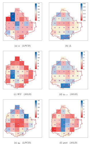
The rainfall recharge factor (β_r) showed significant spatial variability with values ranging from 0.07 to 0.21 with a mean of 0.13 (Table 1). These estimates are very close to our earlier estimate (β_r = 0.135) using the simpler WTF method (Sekhar et al. 2017). Higher values of β_r were observed in grids with less built-up area, which is also consistent with Sekhar et al. (2017).

β_l showed a range of 0.43 to 0.67 with a mean value of 0.53. This factor combines leakage from both water and wastewater systems. For comparison, BWSSB water accounts from September 2013 estimate leakage losses from water supply alone at 37.7%.

λ varied from 0.9 to 0.95 with a mean value of 0.94. A value of 1 for λ means that the entire groundwater column (above h_min) will become base-flow in unit time step and a value of 0 represents zero baseflow for any groundwater level. h_min showed a range of 750 to 885 m with a mean value of 841 m. A significant correlation was observed between h_min and elevation of the grid with a Pearson correlation coefficient of 0.78.

Estimated fluxes

City aggregate

Figure 4 presents the mean city-wide estimated water fluxes in scaled context. Table 2 presents the uncertainty in the city-wide aggregated fluxes. Total water use was estimated as 1470 (1431–1499) MLD. The range describes the 25–75 percentile estimates computed using the behavioural ensemble, as described in the Methodology section. Spatial distribution of this total water use is shown in Figure 3. Groundwater pumping meets the majority of this use, at 827 (789–857) MLD, followed by utility water supply, at 643 MLD. Total recharge from all sources was estimated to be 973 (953–993) MLD, with natural recharge accounting for a much smaller portion, 183 (181–184) MLD, compared to anthropogenic recharge from leaking water and wastewater systems of 791 (771–812) MLD. After accounting for base-flow, the city as a whole experienced a net negative groundwater balance at −40 MLD (−69 – −13). Significantly, the total anthropogenic recharge for the city as a whole is quite close in magnitude to total groundwater extraction.

Figure 4. Schematic of the urban water budget. Mean city-wide fluxes are displayed to scale

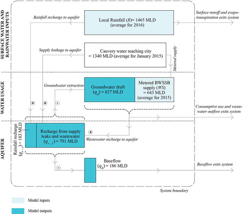
At the city-wide scale, all the fluxes have relatively low uncertainties except net groundwater balance, using Coefficient of Variation (CV) as a measure of uncertainty (Table 2). Groundwater draft has Coefficient of Variation (CV) of 5.8%. Rainfall recharge had lower uncertainty than groundwater draft. Possible under – or over estimation in the uncertainty of the fluxes is described in Section 3.3. Net groundwater balance has a standard deviation very similar to that of total water use and groundwater draft; however, its CV is high because its mean value is low.

The estimated total water use (1470 MLD) is consistent with the independent survey estimate of residential-only demand, which at 2013 population estimates was 977 MLD (Malghan et al. 2018), and scaled to 2016 would be 1033 MLD. A corollary estimate of non-residential demand can thus be made (although only at a city-wide scale) from the difference, at 437 MLD.

Natural recharge estimates are very close to our earlier WTF method-based estimate of 186 MLD (Sekhar et al. 2017). The finding of anthropogenic recharge being much higher than natural recharge from rain is consistent with earlier lumped model estimates (e.g. Mehta et al. 2013, 2014), and reflects the urban water balances of many cities around the world as described in the introduction. A net negative groundwater storage change of 2016 is consistent with our earlier estimate based on the WTF method, which found a larger deficit at 51.6 MLD (Sekhar et al. 2017).

Spatial variation of model estimates

The spatial variation in rainfall recharge q_r−r is presented in Figure 3. Natural, rainfall recharge fluxes follow the pattern of rainfall recharge coefficients (β_r), as expected. A visual comparison with the land-use map (see Figure 2) confirms that ordinal ordering of the grids in terms of rainfall recharge follows the land use patterns. Grid-27 and Grid-28 at southern edge of the city that abuts a reserved forest are also predicted by our model to produce the highest level of rainfall recharge. The central parts of the city, which are most densely built, show the lowest levels of recharge. We see a factor of two variation in recharge rates between built parts of the city and places that are dominated by vegetation.

Figure 3c shows the spatial variation in the estimated WU. A relatively higher WU is observed in the most densely populated area situated close to Rajajinagar and Chamarajpet and relatively lower WU is observed in the periphery of the city. The observed variation is consistent with spatial distribution of population centres (see Figure 2(b)), and spatial variation in surface water availability (see Figure 2(d)). Pumping rates per capita (Figure 3(e) as LPCD) are higher in peripheral areas where the utility piped network is sparse (Figure 2(d)).

Table 3 lists various components of groundwater balance for each grid. q_r−l is observed to be higher where population density is higher and water supply is provided by BWSSB (see Figure 2). Figure 3(f) shows the spatial distribution of the net groundwater balance at the end of the year 2016. Grids lying in the center of the city showed a positive groundwater balance and those lying in the periphery showed a negative groundwater balance. This result is also consistent with our earlier estimates of net groundwater balance based on the WTF method Sekhar et al. (2017).

Table 3. Grid-wise mean water budget in MLD

Grid ID	Grid Name	WU	$q_{r-r}$	$q_{r-l}$	$q_r$	$q_b$	$q_d$	$q_{net}$
1	Ganganahalli	9.9	6	4.3	10.3	2.5	9.2	−1.4
2	Vidyaranyapura	24.5	8.7	11.5	20.1	9.1	16.2	−5.2
3	Yelahanka New Town	28.9	4.1	17	21.1	4	15.2	1.9
4	Agrahara	15.3	7.7	7.1	14.8	2	12.8	0
5	Peenya	42.1	7.6	25.2	32.8	3.5	33.9	−4.5
6	Jalahalli	61.8	6.6	35.3	41.9	6.5	35.4	0.1
7	Hebbal	65.8	7.6	34.9	42.5	0.6	44.4	−2.5
8	Hennur	48.7	7.6	28.4	36	0	40.6	−4.6
9	Channasandra	17.1	7.2	8.6	15.7	4.1	17	−5.4
10	Herohalli	71.9	7.6	45.2	52.9	0.9	53.5	−1.6
11	Rajajinagar	127.9	4	58.3	62.4	6.6	57.9	−2.1
12	Bangalore Palace	84.1	4	39.9	43.9	9.8	27.5	6.6
13	Cooke Town	74.4	3.5	35.8	39.3	5.8	29.2	4.4
14	Krishnarajapuram	56.6	4.9	33.2	38.1	9.4	30	−1.3
15	Kodigehalli	25	6.1	12.9	19	5.2	17.8	−4
16	Bangalore University	43.3	6.1	29	35.1	17.2	18.9	−1
17	Chamarajpet	136.4	6.1	82.9	89	18.7	73.7	−3.4
18	Shantinagar	79.3	6	40	46	13.6	25.9	6.6
19	Domlur	51.4	4.5	24.7	29.2	5.7	20.6	2.9
20	HAL Airport	37	6	16.5	22.5	6.1	19.1	−2.7
21	Whiteeld	20.6	6.1	10.2	16.3	4.4	15.8	−3.9
22	Kengeri	22.8	5	10.3	15.4	8	16.1	−8.6
23	Chikkasandra	71.9	6.5	36.8	43.4	11.2	38.8	−6.6
24	JP Nagar	89.9	6.6	54.2	60.9	11	43.9	6
25	HSR Layout	75.3	7.6	40.4	48.1	0	49.8	−1.7
26	Doddakannelli	21	7.6	10.4	17.9	8.7	16.1	−6.8
27	Kothnur	39.2	10.6	21.1	31.8	6	25.5	0.2
28	Begur	27.6	10.5	16.3	26.9	5.3	22.4	−0.8
	Totals	1470	183	791	973	186	827	−40

Limitations

This study’s limitations stem mainly from the lack of sufficient granular understanding of many aspects of Bengaluru’s coupled social-hydrological system. We used simplifying assumptions which are described below.

Water supply data

We have assumed that water used over and above BWSSB ‘metered and billed’ supply in a 25 km² grid is met through groundwater pumping from within the grid. However, some additional BWSSB water supply exists, that is not captured in the ’metered and billed’ data. Some of this is ‘Non-Revenue Water’ (NRW), while the second could be called ’Used But Not Metered’ (UBNM) water. NRW is water that is ‘metered but not billed‘. NRW is very small – 0.11% of water pumped from the Cauvery river in 2013, and 0.2% of billed water. This difference is too small to impact our results substantially.

The UBNM component consists of water used through unauthorized connections, unmetered public taps and non-functional meters. BWSSB estimated this UBNM component to be 12.38% of the total water supplied within the city in 2013. No spatially disaggregated estimates are available and after September 2013, BWSSB water accounts do not report UBNM. Therefore, we do not include UBNM in our model for 2016.

Although the supply deficit in a particular grid is met through groundwater pumping, this pumping need not be from within the same grid. Water tankers, which depend on groundwater extraction, may be moving water across the grids. There is no systematic information available to address this issue. Similarly, bottled water used within a grid is assumed to be largely from groundwater, which is likely a safe assumption; however, not all bottled water is sourced from the city. The impact of this assumption is likely to be minimal since the residential water use survey from 2013 (Malghan et al. 2018) estimates that the volume of bottled water use in the city is minor compared to other sources.

Effects of lakes

Our modelling framework does not explicitly account for the effects of lakes. Our objective was to sample the city at a sufficient resolution to estimate the groundwater budget at the 25 km² scale, and not to understand the impact of lakes specifically. However, grid level estimates of groundwater fluxes should theoretically reflect the influence of lakes – at least at the resolution of 25 km^{2 –} to the extent that the groundwater measurement network is able to capture these effects. Variogram analysis presented in our earlier paper (Sekhar et al. 2017) suggests that an investigation concerning influence of lakes would need an even denser network of observation wells than we implemented.

Rainfall and recharge

Monthly rainfall data used as model input was based on an average of several stations distributed across the city (described in Sekhar et al. (2017)). We used an average because of the lack of data quality flags in the dataset received, and the temporal inconsistency in data availability among different observation stations. Any errors in this assumption could be artificially compensated for by the rainfall recharge parameterization. However, the qualitative agreement of the spatial rainfall recharge factor with the built-up area lends a measure of confidence that the effect of spatially varying rainfall may not be substantial at the grid and city scale on a monthly time step, especially given that rainfall recharge is estimated to be a small component of total groundwater recharge.

Another limitation of our study is that we have lumped together recharge from leaking wastewater and water supply pipelines. This decision was made to prevent over-parameterization of the model. If a large database of fine scale groundwater level measurements is generated over time, the wastewater and water leakages could be estimated separately using the model and GLUE framework applied in this study.

Conclusions and recommendations

Quantification of the groundwater budget is necessary for effective groundwater management. As in most developing country cities, this is a challenge in urban India given serious data gaps on supply and demand, and inadequate groundwater monitoring. We have demonstrated how groundwater level monitoring at a fine resolution can be used with models to provide useful estimates of the urban (ground) water budget. Given the data gaps, any such estimate of the budget should be accompanied by an assessment of its uncertainty. In this paper, we have developed and applied a novel framework which achieves this objective.

We implemented a dense sampling framework adequate for analysis at a 25 km² grid. For devising neighbourhood scale groundwater management, in a city as heterogeneous as Bengaluru, an even denser sampling frame would be needed. Simultaneously, several types of social and infrastructural data would be needed at the same scale.

An important finding of this study is the large proportion of recharge from leaking water and wastewater systems, reminiscent of findings from several other large cities as noted in the Introduction. Discrimination between water and wastewater leakages will require more detailed investigation, involving additional secondary datasets and primary investigations regarding chemical species that are known to be associated with those sources (Vázquez-Suñé, Sánchez-Vila, and Carrera 2005).

Models are useful for testing future development scenarios, e.g. involving demand growth, treated wastewater reuse, rainwater harvesting and new water supply sources. We are currently working on developing and applying such scenarios.

Recommendations

1. It is unlikely that in the near future, large knowledge gaps in the social hydrology of Indian cities can be filled by government agencies alone. A citizen-science – crowdsourcing experiment placed within a participatory groundwater management context should be explored. A recent example on groundwater quality monitoring from Lebanon provides useful insights, albeit at the scale of a village (Baalbaki et al. 2019).

2. Model verification will need water quality and chemistry investigation. We recommend that government agencies conduct regular sampling. Local universities should be encouraged to include such sampling and analysis in their curriculum and student theses.

3. Simultaneously, more effort must go into mapping the aquifer and aquifer properties. A 2013 report from the CGWB mentioned only 12 exploratory wells, and 9 observation wells, some of which were used to derive hydrogeological parameters (Central Groundwater Board 2013). Challenges include the dense urban environment, and the inability to control when static levels might occur, since pumping times are determined at household/building level. To start with, aquifer tests could be attempted in public parks, other public lands, university campuses and industrial estates.

4. Overall, an institutional framework must be created that can manage these different efforts. Such an institutional framework must include mechanisms for data curation and analysis, converting that to sound policy, and for enforcing regulations stemming from that policy.

Acknowledgements

Research support from the Cities Alliance Catalytic Fund and the Stockholm Environment Institute’s City Health and Well-Being Initiative is greatly appreciated. K. Balakrishnan was supported by the PEAK Urban program, funded by UKRI’s Global Challenge Research Fund. We are grateful to field assistants Sanjeeva Murthy and P. Giriraj, who measured the groundwater levels. Malghan was supported by the Ministry of Housing and Urban Affairs, Government of India, through an IIMB-CoE grant.

Disclosure statement

No potential conflict of interest was reported by the author(s).

Supplementary material

Supplemental data for this article can be accessed here.

Additional information

Funding

This work was supported by the City Alliance Catalytic Fund [CA/CATF/356/01]; Stockholm Environment Institute City Health and WellBeing Initiative [CHeW]; UKRI Global Challenge Research Fund [PEAK Urban Program/ES/P011055/1]; and Ministry of Housing and Urban Affairs, Government of India Grant ID: IIMB-CoE.

References

- Alva, N. 2019. “Every Day, at Least 6 Seek Nod to Dig Borewells in Bengaluru.” The Times of India, 14 February.
- Baalbaki, R., S. H. Ahmad, W. Kays, S. N. Talhouk, N. A. Saliba, and A.-H. Mahmoud. 2019. “Citizen Science in Lebanon—a Case Study for Groundwater Quality Monitoring.” Royal Society Open Science 6 (2): 181871. doi:10.1098/rsos.181871.
- Balakrishnan, K. 2016. “Heterogeneity within Indian Cities: Methods for Empirical Analysis.” PhD diss., University of California, Berkeley.
- Beck, H. E., N. E. Zimmermann, T. R. McVicar, N. Vergopolan, A. Berg, and E. F. Wood. 2018. “Present and Future Köppen-Geiger Climate Classification Maps at 1-km Resolution.” Scientific Data 5 (1): 180214. doi:10.1038/sdata.2018.214.
- Beven, K., and A. Binley. 1992. “The Future of Distributed Models: Model Calibration and Uncertainty Prediction.” Hydrological Processes 6 (3): 279–298. doi:10.1002/hyp.3360060305.
- Brassington, F. C. 1990. “Rising Groundwater Levels in the United Kingdom.” Proceedings of Institution of Civil Engineers. Part 1 88 (6): 1037–1057. doi:10.1680/iicep.1990.11616.
- Brassington, F. C., and K. R. Rushton. 1987. “A Rising Water Table in Central Liverpool.” Quarterly Journal of Engineering Geology and Hydrogeology 20 (2): 151–158. doi:10.1144/GSL.QJEG.1987.020.02.05.
- BWSSB. 2012. “Annual Performance Report 2011–12.” [ Online]. Accessed 26 April 2018. https://bwssb.gov.in/content/about-bwssb-2
- BWSSB. 2017a. “About BWSSB: Overview of the Sewerage System.” [ Online]. Accessed 26 April 2018]. https://bwssb.gov.in/content/about-bwssb-2
- BWSSB. 2017b. “Plans, Roles, Duties and Responsibilities of Chief Engineer (Waste Water Management).” [ Online]. Accessed 26 April 2018. https://bwssb.gov.in/sites/default/files/ss/CE\%20(WWM)\%20English.docx
- Central Groundwater Board. 2013. Ground Water Information Booklet: Bangalore Urban District, Karnataka. Faridabad: Ministry of water Resources, Government of India.
- Central Groundwater Board. 2016. Ground Water Year Book of Karnataka State 2015–2016. Faridabad: Ministry of Water Resources, Government of India.
- CGWB. 2011. “Ground Water Scenario in Major Cities of India.” Technical Report. Central Ground Water Board of India.
- Decker, E. H., S. Elliott, F. A. Smith, D. R. Blake, and F. Sherwood Rowland. 2000. “Energy and Material Flow through the Urban Ecosystem.” Annual Review of Energy and the Environment 25 (1): 685–740. doi:10.1146/annurev.energy.25.1.685.
- DMG. 2011. “Groundwater Hydrology and Groundwater Quality in and around Bangalore City.” Technical Report. Bangalore: Department of Mines and Geology.
- Foster, S., A. Lawrence, and B. Morris. 1998. Groundwater in Urban Development: Assessing Management Needs and Formulating Policy Strategies. Washington, D.C.: World Bank.
- Gattinoni, P., and L. Scesi. 2017. “The Groundwater Rise in the Urban Area of Milan (Italy) and Its Interactions with Underground Structures and Infrastructures.” Tunnelling and Underground Space Technology 62: 103–114. doi:10.1016/j.tust.2016.12.001.
- Government of India. 2011. “Provisional Population Totals, Census of India, 2011.” Chapter 3:27-60. Office of the Registrar General, Ministry of Home Affairs. New Delhi.
- Gilbert, N. 2012. “Water under Pressure: A UN Analysis Sets Out Global Water Management Concerns Ahead of Earth Summit.” Nature 483 (7389): 256–258. doi:10.1038/483256a.
- Goswami, R. 2017. “Hydrosocial Metabolism of Bangalore City: A Comprehensive Study of Urban Water Consumption.” PhD diss., Indian Institute of Management Bangalore.
- Hassan, A. E., H. M. Bekhit, and J. B. Chapman. 2008. “Uncertainty Assessment of a Stochastic Groundwater Flow Model Using GLUE Analysis.” Journal of Hydrology 362 (1): 89–109. doi:10.1016/j.jhydrol.2008.08.017.
- Hayashi, T., T. Tokunaga, M. Aichi, J. Shimada, and M. Taniguchi. 2009. “Effects of Human Activities and Urbanization on Groundwater Environments: An Example from the Aquifer System of Tokyo and the Surrounding Area.” Science of the Total Environment 407 (9): 3165–3172. doi:10.1016/j.scitotenv.2008.07.012.
- Hegde, G. V., and K. C. Subhash Chandra. 2012. “Resource Availability for Water Supply to Bangalore City, Karnataka.” Current Science 102 (8): 1102–1104.
- Hurst, C. W., and W. B. Wilkinson. 1986. “Rising Groundwater Levels in Cities.” Geological Society, London, Engineering Geology Special Publications 3 (1): 75–80. doi:10.1144/GSL.ENG.1986.003.01.07.
- Jaglin, S. 2014. “Rethinking Urban Heterogeneity.” In The Routledge Handbook on Cities of the Global South, edited by Susan Parnell and Sophie Oldfield, 434–446. Abingdon: Routledge.
- Kennedy, C., J. Cuddihy, and J. Engel-Yan. 2007. “The Changing Metabolism of Cities.” Journal of Industrial Ecology 11 (2): 43–59. doi:10.1162/jie.2007.1107.
- Kim, Y.-Y., K.-K. Lee, and I. Sung. 2001. “Urbanization and the Groundwater Budget, Metropolitan Seoul Area, Korea.” Hydrogeology Journal 9 (4): 401–412. doi:10.1007/s100400100139.
- KSPCB. 2013. A Report of Monitoring Committee on Performance of Wastewater Treatment Plants in the Apartments and Other Establishments in BBMP Limits of Bangalore. Bangalore: Karnataka State Pollution Control Board.
- Kumar, S., M. Sekhar, D. V. Reddy, and M. Kumar. 2010. “Estimation of Soil Hydraulic Properties and Their Uncertainty: Comparison between Laboratory and Field Experiment.” Hydrological Processes 24 (23): 3426–3435. doi:10.1002/hyp.7775.
- Lerner, D. N. 2002. “Identifying and Quantifying Urban Recharge: A Review.” Hydrogeology Journal 10 (1): 143–152. doi:10.1007/s10040-001-0177-1.
- Malghan, D., S. Lele, V. K. Mehta, G. Taneja, D. Sharma, A. Nehra, and R. Goswami. 2018. Source-disaggregated Domestic Water Consumption Patterns in Bengaluru, India. Bengaluru: Ashoka Trust for Ecology and Environment (ATREE).
- Maréchal, J.-C., B. Dewandel, and K. Subrahmanyam. 2004. “Use of Hydraulic Tests at Different Scales to Characterize Fracture Network Properties in the Weatheredfractured Layer of a Hard Rock Aquifer.” Water Resources Research 40 (11). doi:10.1029/2004WR003137.
- Mehta, E. K.-B., R. Goswami, S. Muddu, and D. Malghan. 2013. “Social Ecology of Domestic Water Use in Bangalore.” Economic and Political Weekly 48 (15): 20–30.
- Mehta, R. G., E. Kemp-Benedict, S. Muddu, and D. Malghan. 2014. “Metabolic Urbanism and Environmental Justice: The Water Conundrum in Bangalore, India.” Environmental Justice 7 (5): 130–137. doi:10.1089/env.2014.0021.
- Misra, S., and B. Goldar. 2008. “Likely Impact of Reforming Water Supply and Sewerage Services in Delhi.” Economic and Political Weekly 43 (41): 57–66.
- Narain, S., and P. Pandey. 2012. Excreta Matters: How Urban India Is Soaking up Water, Polluting Rivers and Drowning in Its Own Waste. New Delhi: Centre for Science and Environment.
- Park, E., and J. C. Parker. 2008. “A Simple Model for Water Table Fluctuations in Response to Precipitation.” Journal of Hydrology 356 (3): 344–349. doi:10.1016/j.jhydrol.2008.04.022.
- Planning Commission. 2013. Twelfth Five Year Plan (2012–2017). New Delhi: Govt of India.
- Raju, K. V., S. Manasi, and N. Latha. 2008. “Emerging Groundwater Crisis in Urban Areas – A Case Study of Ward No.39, Bangalore City.” Technical Report.
- Ruiz, L., M. R. R. Varma, M. S. Mohan Kumar, M. Sekhar, J.-C. Maréchal, M. Descloitres, J. Riotte, S. Kumar, C. Kumar, and J.-J. Braun. 2010. “Water Balance Modelling in a Tropical Watershed under Deciduous Forest (Mule Hole, India): Regolith Matric Storage Buffers the Groundwater Recharge Process.” Journal of Hydrology 380 (3): 460–472. doi:10.1016/j.jhydrol.2009.11.020.
- Schandl, H., and A. Capon. 2012. “Cities as Social-ecological Systems: Linking Metabolism, Wellbeing and Human Health.”Current Opinion in Environmental Sustainability 4 (4): 375–377. doi:10.1016/j.cosust.2012.09.001.
- Sekhar, M., M. Shindekar, S. K. Tomer, and P. Goswami. 2013. “Modeling the Vulnerability of an Urban Groundwater System Due to the Combined Impacts of Climate Change and Management Scenarios.” Earth Interactions 17 (10): 1–25. doi:10.1175/2012EI000499.1.
- Sekhar, M., and M. S. M. Kumar. 2009. “Geo-hydrological Studies along the Metro Rail Alignment in Bangalore.” Technical Report. Technical report, Department of Civil Engineering, Indian Institute of Science, Bangalore, India.
- Sekhar, M., M. S. M. Kumar, and K. Sridharan. 1994. “A Leaky Aquifer Model for Hard Rock Aquifers.” Applied Hydrogeology 2 (3): 32–39. doi:10.1007/s100400050039.
- Sekhar, M., S. K. Tomer, S. Thiyaku, P. Giriraj, S. Murthy, and V. K. Mehta. 2017. “Groundwater Level Dynamics in Bengaluru City, India.” Sustainability 10 (1): 26. doi:10.3390/su10010026.
- Sreelash, K., S. Buis, M. Sekhar, L. Ruiz, S. K. Tomer, and M. Guerif. 2017. “Estimation of Available Water Capacity Components of Two-layered Soils Using Crop Model Inversion: Effect of Crop Type and Water Regime.” Journal of Hydrology 546: 166–178. doi:10.1016/j.jhydrol.2016.12.049.
- Srinivasan, V., S. M. Gorelick, and L. Goulder. 2010. “A Hydrologic-economic Modeling Approach for Analysis of Urban Water Supply Dynamics in Chennai, India.” Water Resources Research 46 (7). doi:10.1029/2009WR008693.
- Subash, Y., M. Sekhar, S. K. Tomer, and A. K. Sharma. 2017. “A Framework for Assessment of Climate Change Impacts on the Groundwater System.” Chap. in Sustainable Water Resources Management, edited by T. Zhang, C. S. P. Ojha, S. Rao, and A. Bardossy, 14. Virginia: ASCE.
- Subramanyam, S. 2011. “BWSSB Trying to Register All the Borewells in Bangalore.” Citizen Matters, 3 November.
- Todd, D. K., and L. W. Mays. 2005. Groundwater Hydrology Edition. Vol. 1625. New Jersey: Wiley.
- Vázquez-Suñé, E., X. Sánchez-Vila, and J. Carrera. 2005. “Introductory Review of Specific Factors Influencing Urban Groundwater, an Emerging Branch of Hydrogeology, with Reference to Barcelona, Spain.” Hydrogeology Journal 13 (3): 522–533. doi:10.1007/s10040-004-0360-2.
- WHO. 1993. Guidelines for Drinking Water Quality. 2nd ed. Geneva: Switzerland.
- Wolman, A. 1965. “The Metabolism of Cities.” Scientific American 213 (3): 178–193. doi:10.1038/scientificamerican0965-178.
- Xiong, L., and K. M. O’Connor. 2008. “An Empirical Method to Improve the Prediction Limits of the GLUE Methodology in Rainfall–runoff Modeling.” Journal of Hydrology 349 (12): 115–124. doi:10.1016/j.jhydrol.2007.10.029.