Uncertainty inherent to a conceptual model StormTac Web simulating urban runoff quantity, quality and control

ABSTRACT

Assessing uncertainties of urban drainage models is important for their applications. While most attention in the literature was paid to large comprehensive models, little has been published about Low-Complexity Conceptual Models (LCCMs). This paper explores the uncertainties inherent to a conceptual, data-based proprietary model StormTac Web, simulating annual urban runoff quantity and quality, and serving here as an example of a LCCM. The analyses were demonstrated for a small urban catchment, Sätra in Stockholm, Sweden, using the Law of Propagation of Uncertainties and Morris screening methods. The results indicate that the uncertainty of the modelled annual runoff quality (about 30%) is greater than that of annual runoff volumes (about 24%), and the latter uncertainties can significantly contribute to the uncertainty in runoff quality. In computations of pollutant loads, the most sensitive inputs were land-use specific parameters, including the annual volumetric runoff coefficients and default pollutant concentrations for various land uses.

KEYWORDS:

• StormTac Web model
• uncertainty
• sensitivity
• urban runoff
• pollutant load

1. Introduction

The development of comprehensive urban runoff models has been recognized as one of the greatest achievements during the first 50 years of innovation in urban stormwater management (Marsalek 2013). As the urban drainage field has evolved from drainage pipe sizing to sustainable management of drainage systems and protection of receiving waters, the leading contemporary computer models have evolved as well to support the planning and design of modern drainage systems (Fletcher, Andrieu, and Hamel 2013).

While most attention in the modelling literature was paid to large complex models and rightly so, it needs to be recognized that there is a broad spectrum of models ranging from simple to complex ones, which are currently used in the municipal drainage practice to fulfill various computational needs. For example, a quick scan of available stormwater models in the Minnesota Pollution Control Agency Stormwater Management Manual (Minnesota Pollution Control Agency (MPCA) 2019) revealed that there were about 50 models dealing with some aspects of urban drainage, and about one-quarter of those could be classified as Low-Complexity Conceptual Models (LCCMs) (also called tools, or calculators), with low demands on input data and other resources. Thus, there is a significant presence of LCCMs in drainage practice, particularly when dealing with planning tasks and the comparison and selection of design options, which would be further developed by comprehensive modelling. Consequently, it is of interest to examine, even semi-quantitatively, the issues of uncertainty inherent to urban runoff modelling with LCCMs.

Approaches to examining the modelling uncertainties differ depending on modelling objectives, which may range from close approximations of field measurements, as commonly applied in research papers, to meeting broader objectives of urban drainage projects (Water Environment Federation (WEF) et al., 2012). In the latter case, the modelling objectives reflecting the needs of modellers and decision makers were summarized by WEF et al. (2012), and a slightly extended version of this summary follows: (a) Regulatory compliance (i.e. acceptance of the modelling procedure and results by the regulatory agency); (b) The model complexity required – as it applies to the hydrologic procedures, i.e. event or continuous modelling, hydrologic abstractions, snowmelt analysis; water quality simulations – parameters, concentrations and loadings; (c) Land use (the type of development); (d) Area to be modelled (the size, spatial detail required); (e) The purpose of modelling – planning, design/analysis, or operation; (e) Temporal scales – while flow simulations may require high temporal resolution (e.g. peak flows), water quality modelling may be done with lower resolutions for events, seasons, or years; (f) Modelling expertise available in the group conducting modelling; and (g) project duration and timing (longer lead times may be needed when collection of calibration data is required).

In the assessment of uncertainty sources in applications of urban drainage models, Deletic et al. (2012) identified nine sources arranged in three groups: (A) model input uncertainties ((i) input data and (ii) model parameters); (B) calibration uncertainties ((iii) calibration data uncertainties, (iv) selection of appropriate calibration input and output linked to the choice of calibrated variables, (v) calibration algorithms, (vi) objective functions used in the calibration process); and (C) model structure uncertainties ((vii) conceptualization errors (scale issues, or omission of key processes), (viii) equations poorly describing the processes, and (ix) numerical methods and boundary conditions).

The preceding general framework of model uncertainties can be applied to LCCMs as well, recognizing three points: (I) A greatly varying nature and structure of LCCMs is likely to influence the significance of the above nine uncertainty sources with respect to individual LCCMs; (II) Direct comparisons of LCCMs against the physically based models may not be feasible in the cases, where the LCCM produces an integrated output (e.g. annual loads of pollutants), which would require a great effort to reproduce with a calibrated complex model; and (III) a general observation by WEF et al. (2012) that greater amounts of uncertainty are inherent to the more complex models requiring calibration.

The aim of the paper that follows is to present a framework for addressing uncertainties in low-complexity conceptual urban runoff models and demonstrate the underlying methodology on one example of such tools, the data-based StormTac Web model, which is currently used in municipal practice in simulations of urban runoff quantity, quality and their control. Specific objectives are to: (1) identify sensitive parameters/inputs of the StormTac Web model, as an example of a LCCM, for a selected test case; (2) quantify uncertainties in model outputs, including annual runoff, pollutant loads and average pollutant concentrations; and, (3) use such information to evaluate and discuss uncertainties inherent to the model inputs and applications.

2. Methods

2.1. Model description

The proprietary model StormTac Web has been developed by StormTac Corporation and used by consulting and construction companies, municipalities, and universities for modelling urban stormwater pollutant loads and their assessment with respect to permitted loads discharged to receiving waters. It is a parsimonious conceptual model, of which complexity was adapted to the scope of input data typically available in different stages of urban drainage projects, ranging from the planning to construction of stormwater management facilities. Thus, only one operative model is needed to address the catchment system analysis, including calculations of stormwater and baseflow and pollutant exports, general impacts on the chemistry of receiving waters, acceptable loads or required load reductions in relation to applicable effluent guidelines, and the design of transport, flow detention and pollutant treatment facilities.

A schematic diagram of StormTac Web is shown in Figure 1 and further described below. The model comprises five interlinked modules, designated on the StormTac website (http://www.stormtac.com, visited on 20 February 2020) as: (1) runoff and baseflow, (2) pollutant transport, (3) stormwater treatment (4) receiving water, and (5) flow detention and transport. The analysis presented here deals only with the performance of the first two modules (Runoff and baseflow and Pollutant transport, see Figure 1), and ‘transport’ is understood here as the assumed movement of runoff and pollutants from the catchment to the outfall, or control facilities.

Figure 1. The model structure of StormTac Web

In simple applications, the model requires limited input data – the catchment area (ha) and land use, and the annual precipitation (mm/yr). Where water quality controls are contemplated, the area and volume of the receiving water body is required to calculate allowed loads to the receiving water body and the required load reductions. Better site-specific runoff volumes and pollutant loads can be obtained by substituting locally measured input data into the model, e.g. pollutant concentrations and precipitation records.

The average annual runoff flow rate, from a catchment consisting of N sub-catchments with individually specific land uses, is calculated by

(1) $Qr=10\cdot p{\sum }_{i=1}^N\left(\phi Vi\cdot Ai\right)/(365\cdot 24\cdot 3.6)$(1)

where $Qr$ refers to average annual runoff flow rate (l/s), $p$ is annual precipitation depth (rain + snowfall) (mm/yr), corrected for specific land use, $\phi Vi$ is the volumetric runoff coefficient for specific land use i (dimensionless), and $A_i$ is the sub-catchment area (ha).

Using site-specific data, the model calculates the average annual baseflow rate $Qb$ (l/s) at the catchment outlet, attributed to the infiltration and inflow into storm sewers, as a sum of average annual baseflow rates from the individual land-use sub-catchments. For each land-use sub-catchment, such a flow rate is calculated by

(2) $Qb=10\cdot p\cdot \mathrm{K}\mathrm{x}{\sum }_{i=1}^N\left(Kinf,i\cdot Ab,i\right)/(365\cdot 24\cdot 3.6)$(2)

where Q_b is the annual baseflow (l/s), K_x is the fraction of K_inf that contributes to the baseflow (-), K_{inf, i} is the fraction of p that infiltrates into soils (-) for land use i, and A_b,i is baseflow (groundwater) source area (ha) from land use i. In particular, K_inf,i is estimated by

(3) $Kinf,i=\frac{p-\left(p\cdot \phi Vi\right)-Ei}{p}$(3)

where E_i refers to annual potential evapotranspiration (mm/yr) from land use i and can be estimated as a function of land-use specific runoff coefficient (Larm 2000).

The average stormwater runoff pollutant j load L_rj (kg/yr) exported from the catchment is calculated as a sum of runoff pollutant loads from individual land-use sub-catchments, calculated by

(4) $Lrj=1000\cdot {\sum }_{i=1}^N\left(Qri\cdot Cri,j\right)/(365\cdot 24\cdot 3.6)$(4)

where L_rj is the annual load of pollutant j conveyed by stormwater runoff (kg/yr), and Cri,j is default concentration of pollutant j in stormwater runoff from a sub-catchment with land use i (µg/l) (j is the selected pollutant).

Similarly, the annual baseflow pollutant j load, L_b,j is calculated from the baseflow and the land-use specific baseflow concentrations, calculated by

(5) $Lb,j=1000\cdot {\sum }_{i=1}^N\left(Qbi\cdot Cbi,j\right)\cdot /(365\cdot 24\cdot 3.6)$(5)

where L_b,j is the annual baseflow load of pollutant j (kg/yr), and C_bi,j is the default concentration of pollutant j in baseflow from land use i (µg/l).

For specifying volumetric runoff coefficients and pollutant concentrations, the users have two options: (a) select typical values (called here ‘default’ values) from the model documentation, or (b) provide and use their own site-specific data. The concentration data in the StormTac Web database are compiled as annual event-mean concentrations (EMCs) obtained from long periods (at least several months, but preferably 1 year or more) of flow proportional sampling and analysis of stormwater quality.

The total pollutant concentration (C) in storm sewer flow at the catchment outlet is calculated as a flow-weighted average of stormwater and baseflow concentrations, estimated by

(6) $C=\frac{Cr\cdot Qr+Cb\cdot Qb}{Qr+Qb}$(6)

where C is total annual pollutant concentration in storm sewer effluent, representing a mixture of stormwater and baseflow, from the catchment (µg/l).

Calculations of pollutant loads and concentrations in StormTac Web are based on land-use specific concentrations (Larm 2000), with significant differences in concentrations in different land-use categories, as also reported by Pitt, Maestre, and Morquecho (2004). It should be noted that in StormTac Web, more than 70 water quality parameters can be considered, with default concentration data provided for more than 100 land uses. The groups of water quality parameters include nutrients, heavy metals, suspended solids and various organic compounds, specified for such types of land use as residential areas of various densities (e.g. townhouses, apartment blocks), thoroughfares (roads), commercial areas, industrial areas, parks, meadows, forest and agricultural lands, etc., with options allowing the model users to further define and customize such selections.

2.2. Sensitivity and uncertainty analyses

As noted by Kavetski, Kuczera, and Franks (2006), computer models of environmental systems represent crude approximations of actual complex conditions, and their performance can be increased by a number of actions including calibration, determination and segregation of sources of uncertainty, model sensitivity analysis, and reducing input data error bias. One of the objectives of this paper is to examine the applicability of such actions to StormTac Web, for which the modelled processes can be divided into two broad categories: the catchment hydrology and runoff quality.

The first category, urban hydrological processes, has been studied fairly extensively (e.g. as reviewed by Deletic et al. (2012)) and a relatively good understanding of such processes has been developed, particularly in the catchments, of which hydrology is dominated by impervious parts of the catchment. StormTac Web input data for runoff computations are relatively simple (Table 1 and Equations (1)(1) $Qr=10\cdot p{\sum }_{i=1}^N\left(\phi Vi\cdot Ai\right)/(365\cdot 24\cdot 3.6)$(1) –(3(3) $Kinf,i=\frac{p-\left(p\cdot \phi Vi\right)-Ei}{p}$(3) )): the annual precipitation (mm/yr), catchment (sub-catchment) area (ha), and potential evapotranspiration (mm/yr). The main sources of uncertainty in runoff and baseflow calculations include annual volumetric runoff coefficients (specified for the whole year, including the winter period with snowfall), and estimation of baseflows (where they occur), involving estimations of infiltration and its fraction contributing to baseflow, and the infiltration source areas.

Table 1. Input data and process parameters in StormTac Web for calculations of water flow and pollutant loads

Category (item No.)	Input Data	Process parameters
Hydrology/runoff
1	P: locally corrected precipitation depth (rain+snow) (mm/yr)	φV: Land-use specific volumetric runoff coefficient (-) for calculation of annual runoff flow and pollutant loads
2	A: (sub)catchment area per land use (ha)	Ab: baseflow (groundwater) contributing area (ha)
3		Kinf: Infiltration coefficient (-) per land use (annual fraction of the precipitation that is infiltrated) for calculation of annual baseflow and baseflow pollutant loads
4		Kx: Fraction of the infiltration coefficient used in calculations of infiltration contributions to the baseflow
Pollutant concentrations in runoff (used in load calculations)
5		C: Stormwater concentration per chemical and land use (µg/l)
6		Cb: Baseflow concentration per chemical and land use (µg/l)

More challenging is the second category, dealing with runoff and baseflow quality. As motivated by the quantification methods of the StormTac Web model (Section 2.1), a set of key model inputs and parameters were selected for uncertainty and sensitivity analyses (summarized in Table 1 and also explained in Section 2.1). They are divided into two classes, input data and process parameters. The values of input data are essentially adopted from authoritative sources, sometimes with minor adjustments (e.g. of the annual precipitation for a specific location). The annual volumetric runoff coefficient ($\phi V$) is an example of a process parameter, as it represents a summary of the catchment hydrological processes on an annual basis. Finally, in conceptual modelling, the user conducts a fair amount of information synthesis by choosing the ‘right’ values of these process parameters, and that is where ‘uncertainty’ enters the overall analysis.

A sensitivity analysis of the StormTac Web model was carried out first and was followed by uncertainty analysis. Such analyses were demonstrated on a small urban test catchment described in Section 2.3. The sensitivity analyses focused on runoff computations and pollutant loads, and addressed all the model parameters associated with these processes (Table 1). We used the Morris Screening method, also called one-step-at-a-time method (OAT) (Welch et al. 1992), which has been widely used in similar studies for evaluating sensitivities of urban drainage models (e.g. Vanrolleghem et al. 2015; Li et al. 2018) . In this approach, in each run only one input parameter is given a new value, with the others held fixed. In our work, the sensitivities of each parameter to the model outputs were carried out by changing the parameter initial value by + 100%, ± 80%, ± 60%, ± 40%, and ± 20%. We did not exam the changes by −100% due to the fact that the values of some parameters are very unlikely to be zero in real cases, for example, catchment areas (A and A_b in Table 1), land-use specific volumetric runoff coefficient (φV) and infiltration coefficient (K_inf).

For uncertainty analysis, the method of the Law of Propagation of Uncertainties (LPU) (Taylor and Kuyatt 1994) was adopted for analyzing the effects of uncertainties in individual input data on model results. Compared to the commonly used Monte Carlo simulations (Deletic et al. 2012), the LPU method is less demanding on computations and easy to use by modelling practitioners. In this aspect, the application of the LPU can be beneficial for LCCMs with respect to such modelling objectives as, e.g, planning, design/analysis and problem screening. A description of the method used for calculation of relative uncertainties follows and is exemplified for calculation of baseflows and stormwater flows.

2.3. Relative uncertainty for products of variables

The baseflow (Q_b) and runoff flow (Q_r) are calculated as products of several independent variables. The resulting percent (%) relative uncertainties ($\delta$) in baseflow ($\delta$ _Qb) and runoff flow ($\delta$ _Qr) were derived from Taylor series expansion by Hedbrant and Sörme (2001) and used in StormTac Web for calculation of the variance of multiplied variables:

(7) ${\delta }_{Qb}=\sqrt{\left({{\delta }_P}^2+{{\delta }_{Kinf}}^2+{{\delta }_{Ab}}^2\right)}$(7)

(8) ${\delta }_{Qr}=\sqrt{\left({{\delta }_P}^2+{{\delta }_{\phi V}}^2+{{\delta }_A}^2\right)}$(8)

2.4. Relative uncertainty for the sum of variables

The total flow (Q_tot) is calculated in StormTac Web as the sum of two variables and its uncertainty is described by Equation (9)(9) ${\delta }_{Qtot}=\sqrt{({(Q_b\cdot {\delta }_{Qb})}^2+\left(Q_r\cdot {\delta }_{Qr}{)}^2\right)}/\left(Q_b+Q_r\right)$(9) , derived by Hedbrant and Sörme (2001) on the basis of Casella and Berger (1990):

(9) ${\delta }_{Qtot}=\sqrt{({(Q_b\cdot {\delta }_{Qb})}^2+\left(Q_r\cdot {\delta }_{Qr}{)}^2\right)}/\left(Q_b+Q_r\right)$(9)

The literature search has not yielded any estimates of uncertainties in annual volumetric runoff coefficients (φ_V in Table 1), and hence further analysis had to rely on assuming such values. Among various urban catchments, there will be still differences in their φ_V values, with the least uncertainties corresponding to the catchments, of which runoff is controlled by directly connected impervious areas (DCIA). In such areas, the only applicable hydrologic abstraction is quasi-constant surface detention storage and the remaining rainwater runs off (Marsalek et al. 2008). In that case, one could estimate the uncertainty in φ_V as about 14% (assuming identical relative uncertainties in DCIA area and the annual precipitation of 10%). However, in suburban catchments with higher proportions of runoff contributing green areas and snowmelt runoff in winter months the φ_V uncertainties will be higher. Given the above concerns, the uncertainty of φ_V in specific land-use areas was set at 20% in this study.

Infiltration coefficients (K_inf) are in StormTac Web calculated as a function of volumetric runoff coefficients, so they were set to contain the same uncertainties as runoff (20%). The variation in baseflow is smaller than that of stormwater, but it could not be calculated because of lack of data. Some limited data in the StormTac Web database show a variation between 14% and 43% (the normal value of K_x is 0.7, varying from 0.4 to 0.8). Thus, the baseflow coefficients (K_x) were assigned an uncertainty of ±20%. For the concentration data, the relative uncertainty (%) for pollutant event mean concentrations in stormwater and baseflow was estimated at 20% (typically ranging 10–30%) (Bertrand–Krajewski et al., 2002; Francey 2010). While recognizing that pollutant concentration uncertainties may vary among land uses and chemicals, for simplicity, a single value (20%) was assumed to apply in all those cases.

2.5. A case study demonstrating the StormTac Web application and modelling uncertainties

An urban catchment of 26.5 ha in Sätra (further referred to as the Sätra test catchment), located in south-western Stockholm, Sweden, was chosen for a case study of StormTac Web uncertainties (Figure 2). This catchment was selected primarily for two reasons: (i) it represents a mix of land uses and surface covers typical for similar Swedish urban developments, and (ii) the site provided one of the best sources of data on urban runoff flows and quality in Sweden. For investigating stormwater quality, the total concentrations of four water quality parameters were selected: Phosphorus (P), Copper (Cu), Zinc (Zn) and Total Suspended Solids (TSS). These parameters are considered of general environmental importance in various countries and subject to compliance with water quality criteria as a basis for designing stormwater treatment facilities (Larm and Alm 2014).

Figure 2. Map of the studied test catchment Sätra. Orthophoto: Image Landsat Copernicus, Google Earth Pro (obtained for the study period of 1999–2000). The white dotted line indicates the boundary of the catchment area

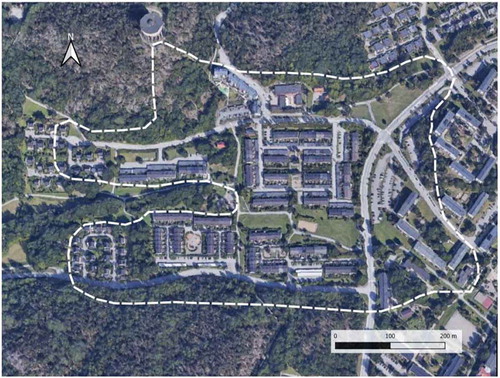
For runoff simulations with StormTac Web, users need to define the runoff contributing area (A) and the groundwater collection area (the baseflow area; A_b) for the study catchment (further explained in Section 2.2). The runoff and groundwater watershed boundaries were assumed to coincide. The detailed information regarding land use areas for the study catchment is presented in Table 2. The share of imperviousness of the catchment (the impermeable surface area/total catchment area) is about 0.39.

Table 2. Land use types and their areas in the Sätra test catchment

	Land uses, i	Runoff and groundwater contributing areas A or Ab (ha)
1	Road area*	0.7
2	Parking	1.0
3	Residential area	2.1
4	Terraced house area	6.5
5	Multi-family area	1.3
6	Park grounds	4.2
7	Forest	10.7
	Total area	26.5

* The road has an average daily traffic (ADT) of 2,700 vehicles/day (used as an input to the StormTac Web model to calculate pollutant concentrations from empirical relationships). The road area contributes only a small amount of groundwater from infiltrated precipitation through the road material and cracks, expressed by a low K_inf-value. ‘Terraced house area’ is the area with terraced buildings, including all land uses within a normal terraced area, such as local streets, ditches, roofs, driveways, small parkings and lawns. ‘Multi-family area’ is the area of multifamily buildings, including all land uses within a normal apartment block area, such as local streets, ditches, roofs, driveways, small parkings and lawns (Larm 2000).

In this study, we adopted the model input data from an earlier study of the Sätra catchment conducted for the period of June 1999 to May 2000 during the initial model development work by Larm (2000). A summary of the adopted values of model inputs together with identified uncertainties is presented in Supplementary Information. The details regarding model simulation for Sätra were presented in Larm (2000), and in this study we focused on using the original data inputs for uncertaity calculation.

In the case of Sätra, the annual precipitation was measured locally as 464 mm during the study period. However, for the Stockholm area (including Sätra), SMHI (Swedish Meteorological and Hydrological Institute) estimated the annual precipitation as 10% higher, at 510 mm, after accounting for errors due to evaporation, wind effects and gauge collector wetting (SMHI 2003). This corrected precipitation was adopted in our study. Furthermore, we estimated the relative uncertainty in annual precipitation as 10%; such an assumption is also supported by Strangeways (2004; estimated as 5–10%). For calculation of the catchment area, we adopted an uncertainty of 10% after Francey (2010). The same assumption was applied to the groundwater area. A common and often justified assumption when studying shallow groundwater systems is that surface and groundwater watershed boundaries coincide (SKB 2003).

3. Results and discussion

3.1. Sensitivity analysis

The sensitivity of water flows, pollutant loads and total concentrations to changes of the selected inputs/parameters (Table 1) were done using the OAT method (Section 2.2). In all the cases of the studied substances, the sensitivities showed similar behaviour. Taking Cu as an example, the results for annual average water flow, total Cu load and total Cu concentration are presented in Figure 3. For brevity, the results for the other chemicals were not shown.

Figure 3. Sensitivity analyses of annual water flow (a), total Cu loads (b) and total Cu concentration (c) to changes of the selected model inputs/parameters. The selected model inputs/parameters were explained in Table 1. The reference values (0%) of the varied parameters: p = 510 mm/yr; Kx = 0.7; ϕ_v ranges from 0.05–0.85 for different land uses; A and Ab range from 0.7–6.5 ha; C ranges from 6.5–40 µg/l, C_b ranges from 4.0–13 µg/l and K_inf = 0.09 (also shown in Table S1 in supplementary information)

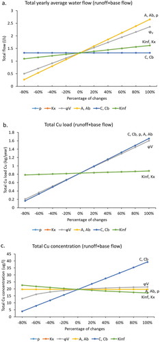
The results in Figure 3(a) suggested that (sub)watershed area per land use (A in Table 1), baseflow (groundwater) area (A_b) and precipitation intensity (p) were the three most sensitive inputs in calculating total annual water flows (runoff + baseflow), closely followed by the second most sensitive parameter, land-use specific volumetric runoff coefficients (φ_V). Two other hydrological parameters, the infiltration coefficient (K_inf) and the fraction of the infiltration contributing to the baseflow (described by K_x), were found to be less sensitive compared to land-use specific volumetric runoff coefficients. This indicated that good quality control for the data inputs of land-use area and precipitation are needed, followed by the parameter of land-use specific volumetric runoff coefficient when using the StormTac Web model.

Regarding the results for the total pollutant loads, as shown by Cu in Figure 3(b), the annual load was rather sensitive to the inputs of default concentrations, land-use areas, precipitation and specific volumetric runoff coefficients. This can be explained by the calculation methods in the StormTac Web model, where the estimation of pollutant loads strongly depends on the inputs of the default concentrations and simulated water flows. Similar to the finding for the total annual drainage water flow, lower sensitivities were also noticed for the parameters of infiltration coefficient (K_inf) and the fraction of the infiltration that reaches the baseflow (K_x).

In contrast to the total Cu loads, the total Cu concentration was found to be most sensitive only to the changes in the default concentrations, while land-use area and precipitation seemed to be less sensitive (Figure 3(c)). This is probably due to the fact that the calculation of the total concentration is based on the pollutant load per unit area and unit water flow. Hence, land-use area and precipitation hardly influence the sensitivity results. In addition, it was noteworthy that the total concentration showed high sensitivity to the changes of volumetric runoff coefficients from −80% to −20%. Taking the value of volumetric runoff coefficient for the road area (0.85) as an example, this variation produces the coefficient values varying from 0.17 to 0.68. In this regard, such negative changes may not be physically realistic for all the parameters. Nevertheless, in general it indicated that care must be taken to choose values of volumetric runoff coefficients in lower ranges for calculating the total concentration.

The total Cu concentration was less sensitive to changes in the two infiltration parameters, (K_inf and K_x (Figure 3(c)). Given that these two parameters determined the baseflow volume and that baseflow Cu concentrations are low, a decreasing trend of the total concentration was shown with the increasing percentage of changes in the two parameters. As the total concentration by definition is calculated by dividing the total loads by the water flow volume, the results also implied the effects of second-order interactions among model parameters with respect to understanding the parameter sensitivity (Knighton et al. 2016).

3.2. Uncertainty analysis of modelling results

Using the method of error propagation (Section 2.2), the results of the uncertainty analysis for annual water flows, pollutant loads and total concentration for Sätra during the studied period are shown in Table 3. The studied annual flows included the baseflow, the runoff flow and the total flow. The investigated pollutants were P, Cu, Zn and TSS. Their annual loads and total concentrations were calculated by the StormTac Web model. Both their absolute and relative uncertainties are presented in the result report produced by the model.

Table 3. Modelling results and estimated uncertainties of the annual water flow, total concentration of pollutant loads and concentrations for Sätra catchment during the study period

Output	Notation	Unit	Calculated results	Calcualted relative uncertainty %*
Baseflow	Qb	l/s	0.29	24
Runoff flow	Qr	l/s	1.0	24
Total flow	Qtot	l/s	1.3	20
Load, baseflow, phosphorus	Lb,P	kg/yr	0.37	32
Load, runoff, phosphorus	Ld,P	kg/yr	6.0	32
Total load, phosphorus	Ltot,P	kg/yr	6.4	30
Total concentration, phosphorus	Ctot,P	µg/l	150	36
Load, baseflow, copper	Lb, Cu	kg/yr	0.050	32
Load, runoff, copper	Ld, Cu	kg/yr	0.77	32
Total load, copper	Ltot, Cu	kg/yr	0.82	30
Total concentration, copper	Ctot, Cu	µg/l	20	36
Load, baseflow, zinc	Lb, Zn	kg/yr	0.18	32
Load, runoff, zinc	Ld, Zn	kg/yr	2.4	32
Total load, zinc	Ltot, Zn	kg/yr	2.6	29
Total concentration, zinc	Ctot, Zn	µg/l	63	35
Load, baseflow, total suspended solids	Lb, TSS	kg/yr	81	32
Load, runoff, total suspended solids	Ld, TSS	kg/yr	2 000	32
Total load, total suspended solids	Ltot, TSS	kg/yr	2 100	30
Total concentration, total suspended solids	Ctot, TSS	µg/l	50 000	36

* The relative uncertainty of model results was calculated by Equations (7)(7) ${\delta }_{Qb}=\sqrt{\left({{\delta }_P}^2+{{\delta }_{Kinf}}^2+{{\delta }_{Ab}}^2\right)}$(7) –(9(9) ${\delta }_{Qtot}=\sqrt{({(Q_b\cdot {\delta }_{Qb})}^2+\left(Q_r\cdot {\delta }_{Qr}{)}^2\right)}/\left(Q_b+Q_r\right)$(9) ), using input uncertainties described in Section 2.2. The total relative uncertainty (%) for a parameter that is a sum, e.g. total flow, is calculated according to a function for summing uncertainties, see Equation (9)(9) ${\delta }_{Qtot}=\sqrt{({(Q_b\cdot {\delta }_{Qb})}^2+\left(Q_r\cdot {\delta }_{Qr}{)}^2\right)}/\left(Q_b+Q_r\right)$(9) . This yields a lower total uncertainty than the respective relative uncertainty for e.g. the baseflow and the runoff flow, respectively. To calculate a relative uncertainty for a parameter, e.g. runoff flow, which is calculated as a product of different parameters, e.g. annual precipitation, volumetric runoff coefficient and the catchment area, another function is used (Equation (8)(8) ${\delta }_{Qr}=\sqrt{\left({{\delta }_P}^2+{{\delta }_{\phi V}}^2+{{\delta }_A}^2\right)}$(8) ) which instead gives higher relative uncertainty than each of the individual parameters (Hedbrant and Sörme 2001).

The relative uncertainties of pollutant loads and concentrations were determined by using Equations (7)(7) ${\delta }_{Qb}=\sqrt{\left({{\delta }_P}^2+{{\delta }_{Kinf}}^2+{{\delta }_{Ab}}^2\right)}$(7) –(9(9) ${\delta }_{Qtot}=\sqrt{({(Q_b\cdot {\delta }_{Qb})}^2+\left(Q_r\cdot {\delta }_{Qr}{)}^2\right)}/\left(Q_b+Q_r\right)$(9) ) together with the assumed input uncertainties, described in Section 2.2. Overall, the uncertainties of the quantified pollutant loads and concentrations simulated by the StormTac Web model were found to be higher than those of calculated water flows. For example, the relative uncertainties of water flows, including the baseflow and the runoff flow were estimated to be 24%, whereas the relative uncertainties of the pollutant concentrations and loads were quantified to be greater than 30%.

The calculated uncertainty of the modelled water flows seemed comparable with the values identified in previous relevant literature on flow measurements. For instance, flow uncertainties of 2–20% in using velocity-area methods have been reported in literature depending heavily on the equipment and the flow conditions (Harmel et al. 2002) and to >30% by Ahyerre et al. (1998). In addition, the indication of a higher uncertainty in water quality than water quantity is in line with previous similar studies on urban drainage models. Vezzaro et al. (2015) tested an integrated dynamic model against micro pollutant concentration measurements and found that the catchment quality submodel showed greater uncertainty than the quantity submodel. In a previous study on comparing different methods for urban water quality modelling by Vanrolleghem et al. (2015), it was emphasized that water quality-related factors in general exerted more important interactions than factors related to water quantity. Indeed, as illustrated in our work on the StormTac Web, the quantification on pollutant loads involves the uncertainties in pollutant concentrations together with the uncertainties in water flows, which further increases the uncertainty in water quality compared with water quantity.

Further, the results implied that the uncertainty analysis of water quantity may contribute as a major part of uncertainty in pollutant loads in the StormTac Web model. In the model, pollutant loads were estimated by multiplying water flow with default concentration. The uncertainty of pollutant loads was calculated as 31%, while the uncertainty of the water flow was already up to 24% according to our study. This agrees with conclusions from many previous studies. For example, Vezzaro and Mikkelsen (2012) highlighted the importance of considering hydrological parameters as a source of uncertainty when estimating the Cu loads for an urban catchment through combining Global Sensitivity Analysis (GSA) with the Generalized Likelihood Uncertainty Estimation (GLUE) technique. In our case using the StormTac Web model, the water flow was calculated based on precipitation and volumetric runoff coefficient. As the former input is usually reliable and has a lower uncertainty; thus, the runoff coefficient seemed to be one the main source of introducing uncertainty to hydrological simulations.

Specifically, for water quality, the results provided by the StormTac Web model also suggested a slightly lower uncertainty for the pollutant loads (around 30%) than that of the total concentration (around 35%) for all the studied substances. This is due to the fact that the calculation of pollutant concentration takes into account the uncertainties in water flows, which introduces extra uncertainty in estimating the total concentration (see Equation (6)(6) $C=\frac{Cr\cdot Qr+Cb\cdot Qb}{Qr+Qb}$(6) ).

In addition, the uncertainties in total concentrations for all the studied pollutants in Sätra were calculated to be 35–36% (Table 3). Comparing our results with the available literature, studies in Europe have recommended an experimental uncertainty of 30% for calculating long-term TSS loads (Bertrand–Krajewski et al., 2002). The level of uncertainty for Cu reported here seems slightly smaller than those determined in an earlier study of a Swedish catchment with an integrated dynamic urban drainage model SEWSYS (Lindblom, Ahlman, and Mikkelsen 2011). In their results, the uncertainty of site mean concentrations was estimated to be 40% for Cu. The same authors, in another case study, showed that the uncertainty in the modelled Cu load was around 50% and emphasized that such a large uncertainty should be acknowledged when referring to pollutant loads modelled by dynamic models, even when site-specific concentrations are used in model calibrations (Lindblom, Ahlman, and Mikkelsen 2007). Dynamic models produce much more detailed data than LCCM models. However, the LCCM models might have an advantage in providing comparable uncertainties by proper control of data inputs, if the focus is on annual values. As demonstrated by the StormTac Web model, this requires better data control of the default pollutant concentrations together with the volumetric runoff coefficient.

3.3. Uncertainties inherent to model inputs and applications

As presented in the uncertainty and sensitivity analyses, annual precipitation (p) was suggested as one of the sensitive inputs when calculating the total drainage water flows and total pollutant loads by the StormTac Web model, while the default concentrations (C and C_b) were the most sensitive inputs when estimating the total pollutant loads and total concentrations. The relative uncertainty (%) for annual precipitation (mm/yr) in this study was estimated at 10%, which is within the range suggested e.g. by Strangeways (2004), 0–10%.

Sources of uncertainties in pollutant concentrations depend on uncertainties in flow measurements and sample analyses. The second source varies depending on the pollutant analyzed. The reported ranges of uncertainties in measured pollutant concentrations varied between 10 and 30%, with TSS (or SS) reported closer to the lower limit (Ahyerre et al. 1998; Bertrand–Krajewski et al., 2002; Harmel et al. 2006) and pollutants primarily transported with solids and requiring more intricate analyses (e.g. trace metals, PAHs) reported closer to the upper limit (Karlsson and Viklander 2008; Francey 2010; Karlsson et al. 2010). In this study, the relative uncertainty of pollutant concentrations (C and C_b) in stormwater was estimated as 20%, which was the midpoint of the overall interval, and for simplicity, such an estimate was assumed to be valid for all land uses and substances. This assumption was also extended to baseflow concentrations, even though they generally vary less than those in stormwater, but there is a lack of data on baseflow concentrations per various land uses, compared stormwater concentrations (StormTac Database 2020).

The simplicity of LCCMs operation provides one specific advantage – they can be used by urban catchment managers with minimum training. Taking the StormTac Web model as an example of such models, this study and practical experience show that with good quality control of model input data, and within the realm of their applicability, the LCCM models may offer comparable levels of uncertainty, in terms of simulating annual runoff flows and pollutant concentrations and loads (Table 3), as complex dynamic models. In this context, Dotto, Deletic, and Fletcher (2009) reported that urban drainage models can be simplified without losing modelling accuracy. In their work, they investigated the MUSIC model (widely used in Australian stormwater practice) and found that only 2 out of 13 calibration parameters of the rainfall/runoff model matter; the model results were insensitive to the remaining 11 parameters.

As shown in this study, catchment area, precipitation, runoff coefficients and default concentrations are the three most important inputs in the application of the StormTac Web model. The LCCMs may avoid introduction of additional uncertainties caused by over-parametrization and excessive temporal detail, compared with high complexity urban drainage models. However, in some applications, e.g. when addressing acute toxicity of stormwater, detailed dynamic water quality data may be needed. Regarding the complex urban drainage models, most information on sensitive parameters and uncertainties was published for simulating runoff flows and quality with the SWMM model. Such studies reported that systematic and random errors in rainfall inputs, model parameters in runoff quality processes (e.g. solids build-up and wash-off), runoff generation parameters (e.g. the directly connected impervious area), and pollutant routing in storm sewers (e.g. the initial depth of in-sewer deposits), have all been identified as sensitive parameters that can all strongly contribute to modelling uncertainties (e.g. Kanso, Chebbo, and Tassin 2005; Kleidorfer et al. 2009; Dotto et al. 2011a, 2011b; Wijesiri et al. 2016; Gorgoglione et al. 2019). Previous studies also implied that it is difficult to identify sensitive SWMM parameters, as they can be case specific and dependent, and there is no set of globally sensitive parameters (Knighton et al. 2016).

Recognizing that annual precipitation data are available from national hydrometeorological agencies and annual volumetric runoff coefficients can be verified by applications of other simple methods (e.g. the SCS Runoff Curve Number Method), the most challenging in applications of StormTac Web is the determination of the land-use specific default concentrations of different pollutants. Consequently, these concentrations are also one of the main sources of uncertainties. Indeed, previous studies indicated that there were significant differences in stormwater constituent concentrations for different land-use categories (Pitt, Maestre, and Morquecho 2004). StormTac Web relies on the dataset of land-use specific concentrations obtained from monitoring campaigns and existing literature. The data management and control should take into account local variations (e.g. climate) for further model development and application. For example, it is well recognised that pollutant concentrations can change under different local climate (e.g.Vezzaro and Mikkelsen 2012). Another work on stormwater quality using the HSPF model indicated that the most sensitive parameters were all linked to soil and land-use characteristics (Fonseca et al. 2014).

The present study represents the first step toward understanding the uncertainties inherent to LCCMs, using the StormTac Web as an example. It should be kept in mind that when carrying out uncertainty analysis, the same percentage of changes in the default pollutant concentrations were assumed for all the land-use types and substances, and the same approach was applied to the annual volumetric runoff coefficients. To obtain more reliable results, future work needs to take into account potential variations of uncertainties with respect to different pollutants and land uses.

4. Conclusions

The assessment of sensitivity and uncertainties of a Low-Complexity Conceptual Model (LCCM) simulating urban runoff quantity and quality, StormTac Web, was carried out for a small urban test catchment, Sätra, in Stockholm, Sweden. The model estimates annual volumes of runoff and baseflow, and annual concentrations and loads of a set of pollutants, using mostly commonly available input data. Among such inputs, three types are particularly important: annual precipitation, annual volumetric stormwater runoff coefficient, and typical land-use specific concentrations of pollutants in stormwater. The sensitivity analysis was done by applying the Morris screening method and the uncertainty analysis was carried out using the Law of Propagation of Uncertainties (LPU).

The study results indicated uncertainties in annual runoff flows (in litres/s) about 24%, and in annual pollutant concentrations and loads about 30%, for total phosphorus, copper, zinc and suspended solids. In simulations with the StormTac Web model, area per land use, precipitation, and land-use specific volumetric runoff coefficients (φ_V) were sensitive inputs for calculating the total runoff flows, and for simulating total pollutant loads, besides the runoff volumes, the land-use specific (default) pollutant concentrations were most important. Among the inputs exerting limited influence on modelling results, one can name the hydrological parameters (K_x and K_inf) controlling the baseflow volume.

Comparison of the StormTac Web model results against the literature data indicates the likelihood of uncertainties levels comparable to those reported for complex drainage models dealing with dynamic hydrological and water quality processes within an urban catchment, subject to two constraints: (a) temporally and spatially averaged results are acceptable (i.e. annual exports at the catchment outfall), and (b) the quality of runoff from the modelled catchment is well characterized by the data in the StormTac Web database, or those supplied by the model user.

Disclosure statement

No potential conflict of interest was reported by the author(s).

Supplementary material

Supplemental data for this article can be accessed https://doi.org/10.1080/1573062X.2021.1878240

Additional information

Funding

This work was supported by DRIZZLE Centre for Stormwater Management, funded by Swedish Governmental Agency for Innovation Systems (Vinnova), Grant no. 2016 - 05176.

References

- Ahyerre, M., G. Chebbo, B. Tassin, and E. Gaume. 1998. “Storm Water Quality Modelling, an Ambitious Objective?” Water Science and Technology 37: 205. doi:10.2166/wst.1998.0050.
- Bertrand–Krajewski, J.-L., S. Barraud, and J.-P. Bardin. 2002. “Uncertainties, Performance Indicators and Decision Aid Applied to Stormwater Facilities.” Urban Water 4: 163–179. doi:10.1016/S1462-0758(02)00016-X.
- Casella, B., and R. Berger. 1990. Statistical Inference. Pacific Grove, CA: Wadsworth and Brooks/Cole.
- Deletic, A., C. B. S. Dotto, D. T. McCarthy, M. Kleidorfer, G. Freni, G. Mannina, M. Uhl, M. Henrichs, T. Fletcher, and W. Rauch. 2012. “Assessing Uncertainties in Urban Drainage Models.” Physics and Chemistry of the Earth, Parts A/B/C 42: 3–10. doi:10.1016/j.pce.2011.04.007.
- Dotto, C. B. S., A. Deletic, and T. D. Fletcher. 2009. “Analysis of Parameter Uncertainty of a Flow and Quality Stormwater Model.” Water Science and Technology 60: 717–725. doi:10.2166/wst.2009.434.
- Dotto, C. B. S., A. Deletic, D. McCarthy, and T. Fletcher. 2011a. “Calibration and Sensitivity Analysis of Urban Drainage Models: MUSIC Rainfall/runoff Module and a Simple Stormwater Quality Model.” Australasian Journal of Water Resources 15: 85–94. doi:10.1080/13241583.2011.11465392.
- Dotto, C. B. S., M. Kleidorfer, A. Deletic, W. Rauch, D. T. McCarthy, and T. D. Fletcher. 2011b. “Performance and Sensitivity Analysis of Stormwater Models Using a Bayesian Approach and Long-term High Resolution Data.” Environmental Modelling & Software 26: 1225–1239. doi:10.1016/j.envsoft.2011.03.013.
- Fletcher, T. D., H. Andrieu, and P. Hamel. 2013. “Understanding, Management and Modelling of Urban Hydrology and Its Consequences for Receiving Waters: A State of the Art.” Advances in Water Resources 51: 261–279. doi:10.1016/j.advwatres.2012.09.001.
- Fonseca, A., D. P. Ames, P. Yang, C. Botelho, R. Boaventura, and V. Vilar. 2014. “Watershed Model Parameter Estimation and Uncertainty in Data-limited Environments.” Environmental Modelling & Software 51: 84–93. doi:10.1016/j.envsoft.2013.09.023.
- Francey, M. 2010. “Characterising Urban Pollutant Loads.” PhD thesis, Department of Civil Engineering, Monash University, Australia, February.
- Gorgoglione, A., F. A. Bombardelli, B. J. L. Pitton, L. R. Oki, D. L. Haver, and T. M. Young. 2019. “Uncertainty in the Parameterization of Sediment Build-up and Wash-off Processes in the Simulation of Sediment Transport in Urban Areas.” Environmental Modelling & Software 111: 170–181. doi:10.1016/j.envsoft.2018.09.022.
- Harmel, R., R. Cooper, R. Slade, R. Haney, and J. Arnold. 2006. “Cumulative Uncertainty in Measured Streamflow and Water Quality Data for Small Watersheds.” Transactions of the ASABE 49: 689–701. doi:10.13031/2013.20488.
- Harmel, R. D., K. W. King, J. E. Wolfe, and H. A. Torbert. 2002. “Minimum Flow Considerations for Automated Storm Sampling on Small Watersheds.” Texas Journal of Science 54: 177–188.
- Hedbrant, J., and L. Sörme. 2001. “Data Vagueness and Uncertainties in Urban Heavy-metal Data Collection. Water, Air and Soil Pollution.” Focus 1: 43–53.
- Kanso, A., G. Chebbo, and B. Tassin. 2005. “Stormwater Quality Modelling in Combined Sewers: Calibration and Uncertainty Analysis.” Water Science and Technology 52: 63–71. doi:10.2166/wst.2005.0062.
- Karlsson, K., and M. Viklander. 2008. “Polycyclic Aromatic Hydrocarbons (PAH) in Water and Sediment from Gully Pots.” Water, Air, and Soil Pollution 188: 271–282. doi:10.1007/s11270-007-9543-5.
- Karlsson, K., M. Viklander, L. Scholes, and M. Revitt. 2010. “Heavy Metal Concentrations and Toxicity in Water and Sediment from Stormwater Ponds and Sedimentation Tanks.” Journal of Hazardous Materials 178: 612–618. doi:10.1016/j.jhazmat.2010.01.129.
- Kavetski, D., G. Kuczera, and S. W. Franks. 2006. “Calibration of Conceptual Hydrological Models Revisited: 2. Improving Optimisation and Analysis.” Journal of Hydrology 320 (1–2): 187–201. doi:10.1016/j.jhydrol.2005.07.013.
- Kleidorfer, M., A. Deletic, T. Fletcher, and W. Rauch. 2009. “Impact of Input Data Uncertainties on Urban Stormwater Model Parameters.” Water Science and Technology 60: 1545–1554. doi:10.2166/wst.2009.493.
- Knighton, J., E. Lennon, L. Bastidas, and E. White. 2016. “Stormwater Detention System Parameter Sensitivity and Uncertainty Analysis Using SWMM.” Journal of Hydrologic Engineering 21: 05016014. doi:10.1061/(ASCE)HE.1943-5584.0001382.
- Larm, T. 2000. “Watershed-based Design of Stormwater Treatment Facilities: Model Development and Applications.” Doctoral thesis, Division of Water Resources Engineering, Department of Civil and Environmental Engineering, Royal Institute of Technology, Stockholm, Sweden.
- Larm, T., and H. Alm. 2014. “Revised Design Criteria for Stormwater Facilities to Meet Pollution Reduction and Flow Control Requirements, Also considering Predicted Climate Effects.” Water Practice & Technology 9 (1): 9–19. doi:10.2166/wpt.2014.002.
- Li, J., R. Zhao, Y. Li, and L. Chen. 2018. “Modeling the Effects of Parameter Optimization on Three Bioretention Tanks Using the HYDRUS-1D Model.” Journal of Environmental Management 217: 38–46. doi:10.1016/j.jenvman.2018.03.078.
- Lindblom, E., S. Ahlman, and P. S. Mikkelsen. 2007. “How Uncertain Is Model-based Prediction of Copper Loads in Stormwater Runoff?” Water Science and Technology 56: 65–72. doi:10.2166/wst.2007.748.
- Lindblom, E., S. Ahlman, and P. S. Mikkelsen. 2011. “Uncertainty-based Calibration and Prediction with a Stormwater Surface Accumulation-washoff Model Based on Coverage of Sampled Zn, Cu, Pb and Cd Field Data.” Water Research 45: 3823–3835. doi:10.1016/j.watres.2011.04.033.
- Marsalek, J. 2013. Fifty Years of Innovation in Urban Stormwater Management: Past Achievements and Current Challenges. NOVATECH. Lyon, France: GRAIE.
- Marsalek, J., B. J. Cisneros, M. Karamouz, P.-A. Malmqvist, J. A. Goldenfum, and B. Chocat. 2008. Urban Water Cycle Processes and Interactions. Boca Raton, FL: CRC Press.
- Minnesota Pollution Control Agency (MPCA). 2019. “Available Stormwater Models and Selecting a Model.” November 27. https://stormwater.pca.state.mn.us
- Pitt, R. E., A. Maestre, and R. Morquecho. 2004. The National Stormwater Quality Database (NSQD, Version 1.1). Tuscaloosa: Department of Civil and Environmental Engineering, University of Alabama. February 16.
- SKB. 2003. “The Groundwater’s Regional Flow Pattern and Composition - Significance for Location of the Deep Repository.” SKB Report R-03-01. Swedish Nuclear Fuel and Waste Management. (In Swedish). https://www.skb.se/publikation/20114/R-03-01.pdf
- SMHI. 2003. “Correction of Precipitation according to Simple Climatic Methodology.” Hans Alexandersson. Swedish Meteorological and Hydrological Institute (SMHI), No 111, 2003, Norrköping , Sweden.
- StormTac Database. 2020. “StormTac Database, V. 2020-02-14.” http://www.stormtac.com/
- Strangeways, I. 2004. “Improving Precipitation Measurement.” International Journal of Climatology: A Journal of the Royal Meteorological Society 24: 1443–1460. doi:10.1002/joc.1075.
- Taylor, B. N., and C. E. Kuyatt. 1994. Guidelines for Evaluating and Expressing the Uncertainty of NIST Measurement Results. Gaithersburg, MD: National Institute of Standards and Technology. NIST Technical Note 1297.
- Vanrolleghem, P. A., G. Mannina, A. Cosenza, and M. B. Neumann. 2015. “Global Sensitivity Analysis for Urban Water Quality Modelling: Terminology, Convergence and Comparison of Different Methods.” Journal of Hydrology 522: 339–352. doi:10.1016/j.jhydrol.2014.12.056.
- Vezzaro, L., and P. S. Mikkelsen. 2012. “Application of Global Sensitivity Analysis and Uncertainty Quantification in Dynamic Modelling of Micropollutants in Stormwater Runoff.” Environmental Modelling & Software 27: 40–51. doi:10.1016/j.envsoft.2011.09.012.
- Vezzaro, L., A. K. Sharma, A. Ledin, and P. S. Mikkelsen. 2015. “Evaluation of Stormwater Micropollutant Source Control and End-of-pipe Control Strategies Using an Uncertainty-calibrated Integrated Dynamic Simulation Model.” Journal of Environmental Management 151: 56–64. doi:10.1016/j.jenvman.2014.12.013.
- Water Environment Federation (WEF), American Society of Civil Engineers (ASCE) & Environmental and Water Resources Institute (EWRI). Design of urban stormwater controls. 2012. WEF Manual of Practice No.23, ASCE No. 87. New York, NY: McGraw-Hill Education.
- Welch, W. J., R. J. Buck, J. Sacks, H. P. Wynn, T. J. Mitchell, and M. D. Morris. 1992. “Screening, Predicting, and Computer Experiments.” Technometrics 34: 15–25. doi:10.2307/1269548.
- Wijesiri, B., P. Egodawatta, J. McGree, and A. Goonetilleke. 2016. “Assessing Uncertainty in Stormwater Quality Modelling.” Water Research 103: 10–20. doi:10.1016/j.watres.2016.07.011.