An initial parameter estimation approach for urban catchment modelling

ABSTRACT

Catchment modelling is an effective approach to simulating the rainfall-runoff process. Estimating parameters is challenging in urban catchments with heterogeneous land use land cover (LULC). This paper describes a novel and reproducible approach to initialise the parameters for modelling catchment hydrology. The Alexandra canal catchment, Australia, was selected as the study catchment. A pixel-based LULC map was generated from the catchment’s orbital image using the Deep Learning (DL) techniques. Integrate the LULC map with subcatchment delineation and hydraulic layout, group LULC attributes to compute the area and imperviousness fraction at pixel scale. The distance from each pixel to the subcatchment outlet was vectorised to estimate flow length. The cumulative likelihood and Kolmogorov–Smirnov (KS) were adopted to describe the parameter distributions, evaluate the goodness-of-fit and LULC effect. Results reflect a limited effect of LULC on flow length, and the approach can initialise the parameters for conceptual catchment modelling systems.

KEYWORDS:

• Catchment modelling
• land use land cover (LULC)
• parameterisation
• Deep Learning

Introduction

Today, more than half of the world’s population live in an urban area, and this will increase to 68% in the middle of the twenty-first century, estimated by the United Nations (Department of Economic and Social Affairs, UN 2018). Urban catchment hydrology and hydraulic issues are clearly getting importance and attracted the focus of various stakeholders during the last decades (Schirmer, Leschik, and Musolff 2013; Salvadore, Bronders, and Batelaan 2015; Fletcher, Andrieu, and Hamel 2013). Urbanisation is considered the significant impact on the hydrological process and the major cause of the increased flood damage as the expansion of impervious areas and growing population and economy (Jha et al. 2011; Feng, Zhang, and Bourke 2021; DeFries and Eshleman 2004). Understanding physical principles of water movement regime and interactions between hydrological components in urban environments are difficult and complex, requiring people to constantly update knowledge and invest human resources and capital to satisfy the demands of urban development. As a practical approach, catchment modelling systems can simulate the critical hydrological components that affect the catchment rainfall-runoff process and quantify them for flood risk analysis (Peel and McMahon 2020). The robustness and prediction performance of a catchment rainfall-runoff model depends on the reliability and feasibility of the parameters used to represent the hydrological components of a catchment (Choi and Ball 2002; Ball et al. 2019).

The primary reason for implementing catchment models is the limitation of catchment hydrological measurement techniques (Beven 2012). In recent years, studies to understand the catchment’s spatial patterns distribution and the water interaction within catchment hydrological components are driven by the increased demand for flood risk management, improved resolution of spatial dataset and computation power. However understanding urban catchment hydrology tends to be more challenging in the phase of catchment conceptualisation and parameters initialisation due to the heterogeneous land use land cover (LULC) and intricate hydraulic system (Salvadore, Bronders, and Batelaan 2015; Chen, Hill, and Urbano 2009; Amini et al. 2011). Estimating parameters to simulate catchment runoff generation and routing is an indispensable component of catchment models, where the initial parameters such as area, impervious fraction and flow length play a critical role in configuring and initialising a catchment model. Obtaining reliable data and conducting sufficient data analysis are compulsory tasks for catchment parameterisation. Nevertheless, such datasets like drainage networks and LULC maps are usually inaccessible, and the associated hydrological mechanisms remain elusive. Thus, tricky to initialise the parameters to drive catchment model under the contradiction between data availability, quality and models’ sophistication. To a certain extent, a reliable initial parameter estimation approach can compensate for the model’s instability and inaccuracy caused by data defects, where the LULC features and their connection mechanism to the catchment outlet are important computational elements used by various catchment modelling systems to simulate runoff quantiles and routing (Tokarczyk et al. 2015; Yang and Li 2015; Thomson et al. 2015).

Based on the difference between parameter estimation and optimisation approaches, it is possible to categorise the parameter estimation methods as

• Forward propagation method. Measure, digitise and compute catchment characteristics using hydroinformatics tools or interpreting external datasets (e.g. GIS and remote sensing data) and parameterise the results for catchment modelling systems.

• Backward propagation method. The parameters are inferred through optimisation algorithms to best fit the observed hydrological data. A lower accuracy of the initial parameters is tolerated but need high-quality catchment monitoring data.

Driven by developments in hydroinformatics systems and the availability of remote sensing data, forward propagated initial parameter estimation for distributed catchment modelling systems is experiencing a lively discussion within the modelling community. The approaches that integrate remote sensing data and Geographic Information System (GIS) are being widely adopted by the catchment modelling community to identify catchment spatial characteristics and estimate parameters. For example, Choi and Ball (2002) utilised a GIS database and calibration techniques to predict the spatial parameters for the Stormwater Management Model (SWMM), a catchment modelling system developed by the United States of America Environment Protection Agency (EPA). Gericke and Du Plessis (2012) developed an unconventional GIS spatial modelling tool to estimate the spatial distribution of catchment parameters. Other applications of ensemble hydroinformatics system-based parameter estimation approaches under different catchment scenarios can be found in El Bastawesy, Mohammed, and Nasr (2009), Tien Bui et al. (2019), Alexakis et al. (2014) and El Alfy (2016). It is worth noting that recognising and digitising spatial datasets for urban catchments with complex and massive spatial characteristics is becoming laborious and challenging due to the LULC heterogeneity and variability caused by urbanisation.

Several backward propagated parameters estimation methods have been developed using the samples optimisation and distribution algorithms. The parameters are adjusted in each iteration of the algorithm until single or multiple stopping criteria are satisfied. For example, Thyer, Kuczera, and Bates (1999) and Vrugt et al. (2003) adopted the Shuffled Complex Evolution algorithm to optimise hydrologic parameters of the conceptual catchment model, while the Bayesian method-based parameter uncertainty analysis is presented by Muleta et al. (2013), Hutton et al. (2014) and Xiaoli et al. (2010). Cooper, Nguyen, and Nicell (1997) found that the performance of the calibration method depends on the selected objective function after the evaluation of three global optimisation methods. Another approach to tackle this issue is the Machine Learning approach method. A Random Forest algorithm was proposed by Sireesha Naidu, Pratik, and Rehana (2020) to determine the effect of climate change-related parameters on hydrological response. While Yang et al. (2019), Tjia, Gupta, and Alam (2020) and Shervan et al. (2021) used machine learning (ML) based methods to discover the parameter relationship between model and data. The backward propagated method is essentially a data-driven approach, and its shortcomings are also prominent. First, extensive data for calibration and optimisation is not ubiquitous. Second, the estimated parameters often lack physical meaning, which limits the applicability of the model. Finally, there is a lack of referencing standardised confidence ranges for some inferred parameters such as catchment width and flow length, which weakens the reliability of estimated parameters.

Whatever the single or multiple parameter estimation methods are adopted, it is crucial to ensure that any estimated parameter is guided by consideration of the conditions or changes in the catchment’s hydrologic and hydraulic characteristics and then mapped in the catchment’s perceptual model and parameter values. Computer Vision (CV) technology, a subbranch of artificial intelligence that trains computers to recognise, understand, and interpret visual datasets like videos and images (O’Mahony et al. 2019; Forsyth and Ponce 2002; Voulodimos et al. 2018), has greatly enhanced the capacity data processing and uncertainty analysis. In this paper, a reproducible initial parameter estimation approach is proposed by utilising a Deep Learning (DL) based CV tool and Cumulative Distribution Function (CDF). A significant innovation is to estimate the flow length of the subcatchment based on the catchment semantic classification results of CV at the pixel scale and evaluate the influence of spatial characteristics on its distribution. This referencing parameter system of this paper is SWMM. According to Choi and Ball (2002), SWMM parameters can be categorised as measured and inferred parameters. The remainder of this paper is organised as follows. The section study catchment describes catchment conditions and adopted datasets following the section ‘Introduction’. The methodology shows the workflow of LULC classification and initial parameters estimation. Section ‘Result and discussion’ demonstrates the statistic analysis of estimated parameters with the discussion of the information behind the parameters. The key findings and research limitations are concluded at the end of this paper.

Study catchment

Catchment description

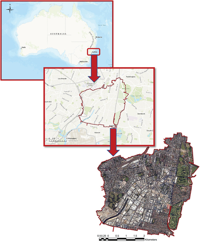
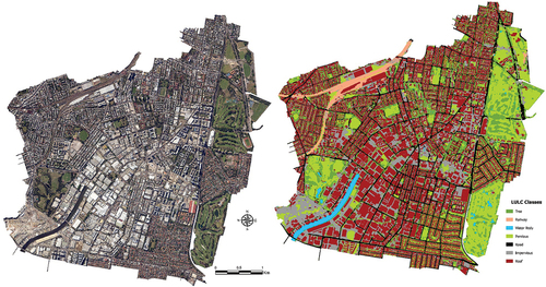
The Alexandra Canal catchment is located south of the Sydney CBD area, Australia, with the total area of 11.50 kilometres square. The catchment is highly urbanised, inclusive of multiple land uses such as residential (approx. 40%), industrial (approx. 25%), road (approx. 10%), parkland (approx. 22%) and water body (approx. 3%). There are heterogeneous land cover types for both impervious and pervious features, including single dwelling, terrace, dense apartment, industrial plants with large impervious areas, and sizeable pervious areas of parkland and golf course. The drainage system of the catchment consists of subsurface pipes, pits, covered channels, open channels, culverts and flood mitigation structures. Shown in Figure 1 is the remote sensing image of the Alexandra Canal catchment with the location respect to continental Australia and within the greater Sydney region.

Figure 1. Location and remote sensing image of Alexandria Canal catchment.

The primary impression of the catchment remote sensing image to people is the high heterogeneous spatial texture and spectral information, such as the various roof colour and shapes, perennial plants, water bodies, railways, walking trails, roads, large pavement areas and buildings’ shadows. Additionally, some catchment areas had experienced changes in land uses, from industrial to commercial or residential, resulting in the discontinuity and failure of existing catchment models and parameters. For example, the control parameter imperviousness fraction of subcatchment is used to compute surface runoff, which is highly dependent on the geometry surveying and mapping of catchment LULC. Therefore, both maintaining the robustness of the existing model and building a new model require the estimation of the relevant parameters due to the change of land uses.

Catchment data

The catchment data used in this research has been obtained from multiple sources for training CV model and estimating parameters, including:

• Remote sensing data

• Subcatchments map

• Stormwater drainage system map

The catchment’s remote sensing data was obtained from the New South Wales Government, Department of Spatial Service, which is a standard RGB (three bands: Red, Green and Blue) image with the resolution of 0.29 meters per pixel width (NSW Spatial Service, 2021). The LULC class schema is defined to represent the catchment’s spatial features, including impervious land, pervious land, railway, road, roof, tree and waterbody. Approximately 25% of the catchment area was selected for training and validation purposes. This area was labelled on the remote sensing image with the defined LULC class schema for preparing the training and validation sets. The ratio of the training and validation sets is 8:2. The remaining 75% catchment area was used as the test set.

The subcatchments delineation (Figure 2) and stormwater drainage maps used in this study are supported by the local government, City of Sydney Council. It is worth noting that, unlike the terrain-based subcatchments delineation, the council uses the control area of drainage networks as the boundaries to subdivide the subcatchments. The drainage-controlled subdivision means the area with ample pits and pipes for collecting and conveying stormwater to the catchment outlet before the water enter the trunk drainage system. The stormwater drainage map covers the information of hydraulic assets belonging to the City of Sydney Council and Sydney Water. A certain degree of simplification of the stormwater drainage map was conducted in this study since the proposed parameter estimation approach in this study is based on the semi-distributed catchment modelling system SWMM. The catchment data and essential data pre-processing are summarised in Table 1.

Figure 2. Subcatchment delineation and outlet.

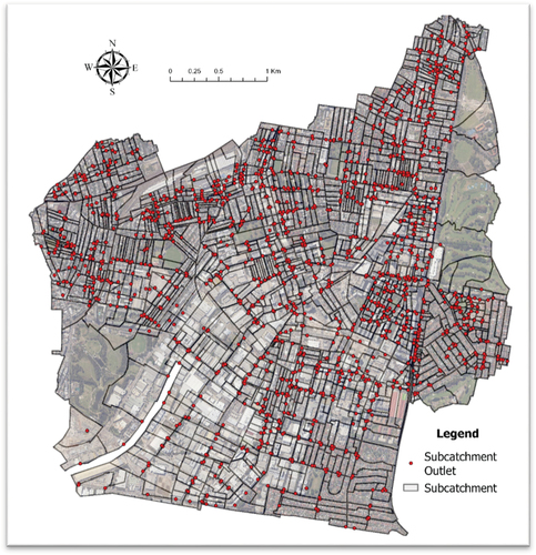
Table 1. Catchment data.

Name	Type	Source	Pre-processing
Remote Sensing Image	RGB Image	NSW Spatial Service	Labelling, Clipping small images (256x256) for the training set
Subcatchments Map	GIS Shapefile	City of Sydney Council	Combine some subcatchments that belong to the same drainage subsystem or depression. There are 1534 subcatchment after merging.
Stormwater Drainage Map	GIS Shapefile	City of Sydney Council	The stormwater pits of one subcatchment with the lowest invert level will be chosen as the subcatchment outlet. Only one outlet was assigned to each subcatchment.

Methodology

Outline of methodology

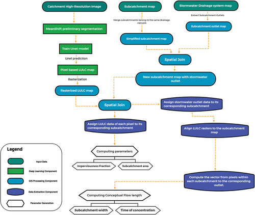
The proposed methods of this paper consist of two parts: the catchment LULC classification and parameters evaluation. The clustering algorithm Meanshift (Cheng 1995) and pixel classifier U-Net (Ronneberger, Fischer, and Brox 2015) were adopted to conduct the LULC classification and segmentation of the catchment remote sensing image. After that, the quantity analysis was applied to evaluate the distribution and tendency of the parameter values generated from the catchment LULC map. A detailed procedure of methodology is demonstrated in Figure 3.

Figure 3. Methodology framework.

LULC Classification and segmentation

The DL techniques and associated CV applications have gained great progress in the recent decade. DL-based CV application with interdisciplinary knowledge by letting the computers acquire information, process data, make predictions and gain advanced understanding from visual images or videos (Szeliski 2010). CV has been widely used to solve classification and segmentation problems of remote sensing related topics and achieved excellent results. Examples of CV be used in remote sensing fields can be found in building footprints extraction (Zhao, Shihong, and Emery 2017), road extraction (Yang and Li 2015) and impervious features segmentation (Huang, Zhao, and Song 2018).

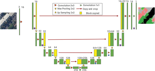
A novel integrated approach utilising a CV tool (U-Net) and clustering algorithm (MeanShift) was adopted to present a semantic segmentation map for Alexandra canal catchment. MeanShift (Comaniciu and Meer 2002), a clustering algorithm, was involved in reducing the spectral and texture heterogenous of the catchment LULC by producing a preliminary object-based segmentation result. U-Net is a classical DL algorithm for semantic segmentation with fully convolutional connections and initiated symmetrical U-shaped structure (encoding and decoding) developed by Ronneberger, Fischer, and Brox (2015), which was first applied to biomedical image segmentation and also achieved excellent performance in the semantic segmentation tasks of remote sensing images (Abdollahi, Pradhan, and Alamri 2022; Cui, Chen, and Yan 2020; Nanjun, Fang, and Plaza 2020). Compared to conventional CV models such as pure U-Net and DeeplabV3 (Chen et al. 2017), the integrated approach has achieved the best accuracy and consistency in predicting LULC of the study catchment (Gong, Ball, and Surawski 2022).

In the beginning, the catchment remote sensing image and GIS data were projected to the WGS1984/UTM zone 56 (the Universal Transverse Mercator projection system) coordinate system. World Geodetic System, or WGS for short, is a widely used geodetic standard in geodesy, navigation and cartography (Eurocontrol, and IfEN 1998). The purpose of georeferencing and unifying GIS data from different sources is to eliminate the error caused by unit system discrepancy. Then, a GIS layer with pre-defined seven representative surface classes (Tree, Pervious, Impervious, Railway, Roof, Road, Water Body) was integrated with the segmented image of MeanShift to generate the training sample. The training sample contains 5460 small image tiles with the size of 256 × 256 for each tile. Following the data training, the output of the MeanShift algorithm was used as the input of the pixel classifier U-Net to produce a pixel base LULC classification and segmentation map. A schematic diagram of U-Net is demonstrated in Figure 4. Finally, the trained U-Net model was applied to catchment raw remote sensing images to make LULC predictions. As prerequisites, the predicted LULC map was rasterised for computing measurable parameters, and the results were conveyed to determine the inferable parameters. Where measurable parameters mean the features are physically measurable such as LULC areas in this study, and the inferable parameters are determined from the measurable attributions, usually have no physical meaning (Choi and Ball 2002).

Figure 4. Structure of U-Net.

Parameters estimation

This paper aims to develop a reproducible approach to estimating initial parameters for catchment modelling systems. With respect to the distributed representative schema of catchment spatial characteristics, three parameters are selected to verify the estimation approach: area, imperviousness fraction, and flow length. Area is the fundamental physical parameter to compute catchment flood quantiles, while imperviousness fraction and flow length are important conceptual parameters to determine the runoff generation and routing. Due to the limitation of monitoring data and measurement techniques, it is necessary to conceptualise some catchment characteristics in the distributed model to simulate the real catchment conditions. Different from the subcatchment focused conceptualisation methods, this paper uses the pixel-based estimation approach to obtain the initial values of the selected two conceptual parameters. Each pixel was assigned and represented by a coordinate, which has been projected to the WGS1984 system at the data preparation stage.

Subcatchment area

A spatial join tool of ArcGIS was adopted to merge the subcatchments delineation layer into the classified LULC raster dataset (pixel snapped) so that it allows to extract raster’s LULC information for each subcatchment. The extracted pixel information are class (C), area (A), and coordinates. Then, the total area and single class area of each subcatchment are expressed as:

(1) $A_i=\sum _1^j{A}_p$(1)

(2) ${ }_{c\left(i\right)}=\sum _0^{j\left(c\right)}{A}_p$(2)

Where $A_i$, $A_p$ and $A_{c\left(i\right)}$ are the total area of subcatchments ‘i’, pixel area and area of LULC class c in subcatchments ‘i’, respectively. ‘j’ is the total number of pixels in subcatchments ‘i’, and ‘j(c)’ is total number pixels belong to class c. The seven pre-defined LULC classes are described in Section 2.1.

Imperviousness fraction

Runoff volume and rates of urban catchments are susceptible to impervious features. A common agreement of computing the total imperviousness fraction in the modelling community is measured total impervious area (TIA) divided by total area, where the TIA is the sum of land uses with impervious feature (Rossman and Huber 2015). In practice, the accuracy of catchment imperviousness fraction relies on the delineation precision of catchment spatial features from remote sensing images, which is time-consuming and tedious. This study conducted a CV-based automatic classification and segmentation of the catchment spatial features instead of humans with higher efficiency and relative precision than manual delineation. According to the catchment spatial features, the LULC classes: roof, impervious land, road and railway are counted to the impervious area, while pervious land and tree belong to the pervious feature. Waterbody does not participate in the calculation, as no contribution of the water body to surface runoff in the study catchment. The equation of TIA and impervious fraction are presented below:

(3) $TI{A}_i=A_{imp\left(i\right)}=A_{roof\left(i\right)}+A_{impland\left(i\right)}+A_{road\left(i\right)}+A_{railway\left(i\right)}$(3)

(4) $F_{imp\left(i\right)}=A_{imp\left(i\right)}/A_i$(4)

Where $A_{imp\left(i\right)}$ and $F_{imp\left(i\right)}$ are the total impervious area and imperviousness fraction of subcatchment i.

Flow length

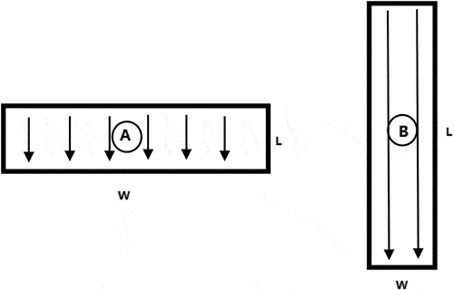
Flow length is a critical parameter to simulate runoff routing in conceptual catchment modelling systems. For example, modellers using SWMM are required to estimate the flow length for computing subcatchment width, which is a conceptual width used to evaluate overland flow rate by assuming a subcatchment shape as rectangular. Two different idealised subcatchments (A and B) shapes with the same area are shown in Figure 5. The side perpendicular to the flow direction is subcatchment width. The side along the flow direction is flow length. The subcatchment B will spend more time to achieve equilibrium on its hydrography than subcatchment A under the same rainfall patterns due to the narrow subcatchment width. A recommended flow length estimation approach by the SWMM manual (Rossman and Huber 2015) is to use the average maximum length (AML) of surface runoff. Maximum length represents the distance from eight selected sample points on the subcatchment boundary to the subcatchment outlet, and the average of the eight distances is considered as the subcatchment flow length.

Figure 5. Schematic of idealised catchment shape to show the relationship between catchment width and flow lengths. W is subcatchment width, L is flow length.

Determine flow length is essential for catchment model and has positive implications for estimating parameters in the absence of extensive data support due to the complexity of runoff routing under actual catchment conditions (Zhou, Minghui, and Chen 2014). In the urban environment, the rainfall-runoff process is affected by multiple factors related to LULC, such as the interactions between pervious and impervious areas, depression and non-depression surfaces, surface runoff and subsurface pipes. Therefore, the flow length estimation methods without considering LULC impact may result in unreliable parameter sets and models in an urban catchment.

As an extension of the SWMM recommended approach, this paper proposed an approach that considers catchment LULC at pixel scale and estimates flow length for subcatchments without the support of an extensive dataset. As mentioned above, the attribution of classified pixel dataset and subcatchment outlet data have been merged to the subcatchment delineation map by aligning their projection coordinate system. In the subsequent steps, the classified two-dimensional LULC pixel network was converted to a dot matrix, where the pixel’s location is defined by the coordinate at the pixel centre. The data are expected from the dot matrix and will be used for computing parameters are:

• Coordinates of dots within the subcatchment.

• Coordinate of subcatchment outlet.

• LULC class information of all dots by referencing to their corresponding pixel.

A new terminology, namely Conceptual Flow Length (CFL), is first proposed in this paper to describe the flow length at the subcatchment scale. Each pixel within the subcatchment is treated as a hydrological unit, and the vector of each pixel reaching the dominating subcatchment outlet is assumed to be the pixel’s CFL. The centroid of pixel CFL within the subcatchment is selected as the representative CFL of the subcatchment by concerning the subcatchment geometry and conceptualised runoff generation process. The subcatchment outlet coordinate is taken as the origin, and each pixel is taken as the mass point to compute the vector. The expression of subcatchment CFL is presented as:

(5) $Vecto{r}_{i\left(j\right)}=\sqrt{\left[{\left(X_{i\left(j\right)}-X_{i\left(o\right)}\right)}^2+{\left(Y_{i\left(j\right)}-Y_{i\left(o\right)}\right)}^2\right]}$(5)

(6) $ConceptualFlowlengt{h}_i=\frac{{\sum }_1^j(Vecto{r}_{i\left(j\right)}\times A_p)}{A_i}$(6)

Where $X_{i\left(j\right)}$ and $Y_{i\left(j\right)}$ are the coordinate of pixel j of subcatchment i. $X_{i\left(o\right)}$ and $Y_{i\left(o\right)}$ is the outlet coordinate of subcatchment i.

Furthermore, the effect of LULC on CFLs is also involved in this study by computing the vector of the pixels grouped by their corresponding LULC feature. The expressions of CFL with LULC are shown below:

(7) $Vecto{r}_{imp/per\left(i,j\right)}=\sqrt{\left[{\left(X_{imp/per\left(i,j\right)}-X_{i\left(o\right)}\right)}^2+{\left(Y_{imp/per\left(i,j\right)}-Y_{i\left(o\right)}\right)}^2\right]}$(7)

(8) $ConceptualFlowlengt{h}_{imp/per\left(i\right)}=\frac{{\sum }_1^j(Vecto{r}_{imp/per\left(i,j\right)}\times A_p)}{A_{imp/per}}$(8)

Where $X_{imp/per\left(i,j\right)}$ and $Y_{imp/per\left(i,j\right)}$ are the coordinate of impervious or pervious pixel j of subcatchment i.

The square root of subcatchment area is raised as the standardised subcatchment width (Std width) to produce a non-dimensional indicator (CFL and Std width ratio) for evaluating the distribution of the CFL. The cumulative likelihood distribution method is applied to generate the distribution curves of the CFL and non-dimensional indicator, which are grouped by different CFL intervals with the same sample amount. The CFL distribution curves are compared to assessing the effect of LULC to subcatchment flow length, while the CFL and Std width ratio curves are used to estimate the initial CFL for urban catchments similar to the LULC conditions of the Alexandra canal catchment. The expression of subcatchment Std width is:

(9) $StdWidt{h}_i=\sqrt{A_i}$(9)

Distribution fitting test

There are 4602 CFL values generated from the 1534 study subcatchments using the aforementioned CFL computation approach. This paper adopts the cumulative likelihood distribution method to describe and analyse the CFL distribution and the impact of different LULC categories on CFL values. The categories are ‘all LULC’ (no consideration of catchment LULC), ‘impervious’ (only account impervious pixels) and ‘pervious’ (only account pervious pixels). Meanwhile, the Kolmogorov–Smirnov test (KS test) was involved in computing the KS statistic for pair-wise comparison of the three categories. The KS test is a classical statistic approach for evaluating the fitting goodness of an empirical and hypothetical distribution or two empirical distributions (Massey 1951). Both KS statistic and p-value (Heyde and Seneta 2001) are computed to assess the fitting of distributions and the significance of statistic difference. The lower the KS statistic, the better the fitting of the two distributions. In contrast, the lower the p-value, the greater the statistical significance of the observed difference. The KS test is also widely used for comparing and evaluating the fitting goodness of catchment model simulations and data distribution. For example, KS statistics was adopted by Wang and Solomatine (2019) to compute sensitivity indices for the cumulative distribution functions of six sensitivity analysis methods. Caballero and Rahman (2013) described rainfall models parameters by probability distributions and tested their fitting goodness with the KS test. A KS test was done by Shahzad et al. (2021) to evaluate the goodness-of-fit of observed flow data and model simulation results. In this case, the expressions of KS statistic for evaluating two samples distribution is

(10) $D_{n,m}=\mathrm{s}\mathrm{u}\mathrm{p}\left|F_1\left(x\right)-F_2\left(x\right)\right|$(10)

where F1 and F2 are the accumulative likelihood distribution functions of the first and second sample, and sup is the supremum function means the absolute value of the maximum difference between F1 and F2.

The distribution of all LULC CFLs are assumed to be a true hypothesis $(H_0)$. Then use the p-value to test the probability of pervious and impervious CFL distributions, which accord with the hypothesis $(H_0)$. The purpose of p-value is to evaluate the effect of LULC on the determination of subcatchment CFL and correlation among them. The expression of p-value is

(11) $\mathrm{p}\mathrm{v}\mathrm{a}\mathrm{l}\mathrm{u}\mathrm{e}=\left\{P_r\left(x\ge t|H_0\right),P_r\left(x\le t|H_0\right)\right\}$(11)

where t is the significance guide numbers 0.001, 0.01 and 0.05 represent extreme significance difference, noticeable significance difference and significance different, respectively (Wasserstein and Lazar 2016).

Results and discussion

Land use land cover map

The catchment LULC map is generated using the MeanShift clustering algorithm and DL-based U-Net model. The sample labelling and training procedure are described in the Section LULC Classification and Segmentation. The confusion matrix approach was applied to evaluate the performance of prediction. For creating the confusion matrix, 500 assessing points were created using the stratified random distribution method, where each class number of assessing points is proportional to its area. An essential modification on this confusion matrix is the combined classes (roof, road, impervious land, railway) with impervious features for fitting the parameter schema of conceptual catchment modelling systems (e.g. SWMM); hence the predicted error within the four classes is ignored. The comparison of catchment raw image and LULC prediction is shown in Figure 6.

Figure 6. Alexandra Canal catchment raw image and LULC prediction.

A further evaluation for LULC map is presented in the confusion matrix Table 2. From this table, the overall accuracy is 0.8953. The prediction accuracy value of the combined ‘Impervious’ class achieved a high accuracy of 0.9847, and the prediction accuracy of ‘tree’, ‘water body’ and ‘pervious land’ are 0.7778, 0.8889 and 0.6804, respectively. The error classification at the lower-left corner of the catchment LULC map (where the ground truth is bare soil) results in lower prediction accuracy for the ‘pervious land’. However, this error has a limited impact on the ‘impervious’ prediction accuracy due to the highly urbanised catchment with a large portion of impervious areas. It is worth mentioning that the runoff generation is susceptible to impervious features (Boyd, Bufill, and Knee 1993; Yang and Li 2015), so that high prediction accuracy of ‘impervious’ could support the estimation of reliable initial parameters and establish a robust catchment model.

Table 2. Confusion matrix of prediction.

Classname	Tree	Water Body	Pervious	Impervious	Total	U_Accuracy
Tree	56	0	7	2	65	0.8615
Water Body	2	8	0	0	10	0.8000
Pervious	7	1	66	3	77	0.8571
Impervious	7	0	24	323	354	0.9124
Total	72	9	97	328	506
P_Accuracy	0.7778	0.8889	0.6804	0.9847

P_Accuracy = Prediction Accuracy

U_Accuracy = User Accuracy

Overall Accuracy = 0.8953

Kappa = 0.7900

Subcatchment area and imperviousness fraction

The LULC map was transmitted to the measured parameters estimation procedure as the fundamental dataset. The governing equations for computing TIA and imperviousness fraction are presented in Equation 3(3) $TI{A}_i=A_{imp\left(i\right)}=A_{roof\left(i\right)}+A_{impland\left(i\right)}+A_{road\left(i\right)}+A_{railway\left(i\right)}$(3) and 4(4) $F_{imp\left(i\right)}=A_{imp\left(i\right)}/A_i$(4) . In this section, two figures (Figure 7 and Figure 8): subcatchments’ imperviousness fraction distribution histogram and accumulated likelihood curve, are plotted to describe the impervious conditions of the 1534 subcatchments. In Figure 7, a few subcatchments have an impervious fraction less than 50% and are distributed uniformly from 0% to 40%. The majority numbers of subcatchments belong to the imperviousness fraction range of 50% to 95%, followed by a significant increase in the range of 95% to 100%. Figure 8 shows the same content in the form of an accumulated likelihood curve; the likelihood curve of imperviousness fraction grows slowly from 0% to 65%, then enters an exponential growth trend with the highest gradient occurring near the curve’s end.

Figure 7. Subcatchments imperviousness fraction distribution histogram.

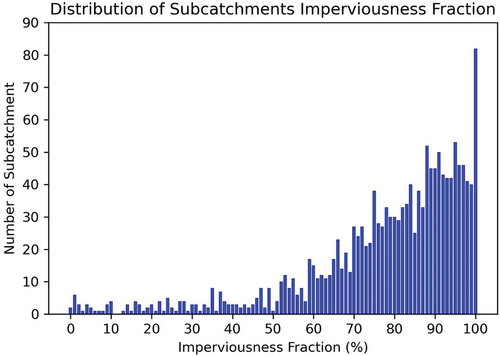
Figure 8. Subcatchments impervious fraction accumulated likelihood curve.

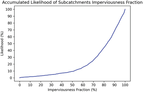
Both Figures 7 and 8 reflected the high urbanisation level of the Alexandra canal catchment with planned impervious developments, where the identifiable industrial, commercial and utility areas from the catchment remote sensing image are the most visible ground surface features. Meanwhile, the significant landscape of residential areas and large urban green spaces also echoes the 30% occurrence likelihood of imperviousness fraction range from 0% to 65%.

Distribution of conceptual flow length and accumulated likelihood

The distribution and accumulated likelihood curves describe the conceptual flow length of the 1534 subcatchments (see Figure 9) including all LULC, impervious and pervious. All LULC classes curve represents the subcatchments’ CFLs without considering the influence of pixels’ LULC attribute. In comparison, the impervious and pervious curves represent the CFLs of subcatchments’ impervious and pervious areas, respectively. No significant difference was observed in Figure 9a by comparing the three types of CFL curves, which illustrates the well-planned proportion of pervious areas in the study catchment, particularly the subcatchment zoned as residential and industrial. Most subcatchments’ conceptual flow lengths are distributed from 25 m to 100 m, which occupies approximately 80% of the total subcatchments number. It is worth mentioning that the three curves climb with the same gradient and reach a peak at 65 meters, then they gradually decrease with similar fluctuations until approaching zero. The erratic fluctuations of the pervious curve between 200 and 500 meters correspond to several subcatchments with ample green space, such as Sydney park and Morre park golf course.

Figure 9. (a) Subcatchments’ conceptual flow length distribution and (b) accumulated likelihood curves of conceptual flow length (1534 subcatchments).

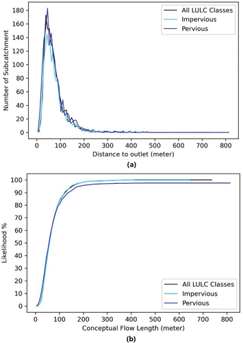
Figure 9b also presents a great similarity of the three curves, where the impervious and all LULC curves almost coincide. The likelihood of three CFLs climb with a similar gradient and approach 100% at 170 meters. The likelihood of pervious CFLs in the range of 170 to 800 meters is lower than the other two curves, revealing impervious dominated LULC of the study catchment, such as the longer CFL of large industrial and commercial subcatchments with high imperviousness fraction than subcatchments zoned to residential.

Table 3 presents the KS test results of the three curves, which further validated the observation from Figure 9a,b from the statistic perspective. The low KS statistic values of pair-wise comparison are not unexpected, which recall the similar distribution observed in Figure 9a,b. All LULC and impervious curves have the best goodness of fit (KS statistic = 0.0156) among the other two comparisons, where the KS statistic of all LULC/pervious and impervious/pervious are 0.0613 and 0.0535, respectively. Corresponding to that, the p-values presents the same kernel of KS statistic. The highest p-value 0.9918 is obtained from all LULC/impervious followed by impervious/pervious 0.0248 and all LULC/pervious 0.0062.

Table 3. KS test and p-values.

	All LULC/Impervious	All LULC/Pervious	Impervious/Pervious
KS statistic	0.0156	0.0613	0.0535
p-value	0.9918	0.0062	0.0248

In summary, both observation and the statistical test proved the excellent goodness of fit for all three pair-wise comparisons, where all LULC/impervious has the highest fitting level and ther is no significant difference between LULCs. In addition, the fitting of impervious and pervious curves illustrates that the landscape area occupies a certain percentage in most subcatchments dominated by residential and commercial land. However, the best fitting of all LULC and impervious further describes the high urbanisation and imperviousness fraction of the Alexandra canal catchment. In this case, the following CFL estimation discussion will focus on the all LULC samples due to the limited impact of different LULC on estimating the CFL of subcatchment.

Estimation of conceptual flow length

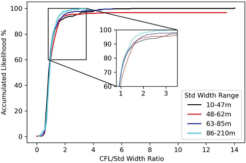
This section focus on the CFLs estimation of all LULC sample due to the limited impact of LULC on CFL values. The Std width (Equation 9(9) $StdWidt{h}_i=\sqrt{A_i}$(9) ) and CFL/Std width ratio are involved in measuring the CFL distribution and testing the CFL estimation approach. The 1534 Std width samples are divided into four different length intervals (10–47 m, 48–62 m, 63–85 m, 86–210 m) to ensure the same sample amount is occurred by each length group. In practical modelling, it is difficult to estimate the CFL value from the CFL likelihood distribution curves due to the difference of subcatchment areas. Therefore, this paper calculates the ratio of CFL to Std width in each subcatchment and summarises it into the corresponding Std width group, then plots the cumulative likelihood distribution curves of each Std width group (Figure 10). Nearly 100% CFL/Std width ratios are lower than 3.5. The four Std width groups present a minor difference from 1 to 3.5. When the area of the subcatchment is known, the modeller can calculate the subcatchment Std width and correspond to the Std group curve in Figure 10 by referring to its length range. The likelihood of CFL/Std width ratio can be obtained from the associated accumulated likelihood curve. Then, the multiply CFL/Std width ratio and Std width to estimate the most likely CFL length.

Figure 10. Accumulated likelihood distribution of CFL/Std width ratio.

This approach can help modellers initialise parameters for catchment modelling systems at the mathematical level without an extensive dataset like ungauged catchment. It is worth mentioning that the sample size is critical to the reliability of the results. Therefore, it is necessary to expand the number of samples in future research to improve the robustness of the results. The subcatchment map used in this study is provided by the City of Sydney Council, where the subcatchment 2D delineation is based on its urban drainage network controlled cadastral map, and most subcatchments are in regular shapes. Therefore, the influence of subcatchment 2D shape on the CFL value determination has not been thoroughly studied. The terrain-based subcatchment delineation method should be adopted to resample the study catchment to further explore the performance of the CFL estimation approach on a different sample system.

Conclusion

This paper proposes an initial parameter estimation approach for distributed catchment modelling systems in the Alexandra canal catchment. The clustering algorithm Meanshift and semantic segmentation neural network U-Net were applied to achieve the pixel based LULC map of catchment remote sensing image. The U-Net model was trained on the preliminary segmentation dataset of Meanshift and made predictions on the remote sensing image to produce the LULC map. Then, the external datasets such as subcatchment delineation map and outlet map were integrated into the LULC map by referring to the spatial coordinate system (WGS1984). The following methods processed the integrated catchment dataset to estimate the initial parameter for catchment modelling.

• Subcatchment area: Use a GIS software package to compute subcatchment area by entering the spatial projection coordinate system (WGS1984).

• Subcatchment imperviousness fraction: Sum the area of pixels with impervious features and divide by the total subcatchment area.

• Subcatchment conceptual flow length: Extract the outlet and each pixel centre’s coordinates of subcatchments. Vectorise the distance from each pixel to the outlet within the subcatchment. Select the centroid value as the subcatchment conceptual flow length by sorting these vectors.

The KS test and cumulative likelihood method were adopted to describe the parameter distributions and evaluate their goodness of fit. The non-dimensional indicator CFL/Std width ratio was computed to plot its accumulated likelihood distribution curves to estimate CFL for an ungauged catchment.

The work contributes to existing knowledge of parameter estimation for catchment modelling, where a comprehensive initial parameter dataset for SWMM was obtained by implementing the above procedure. The results are concluded as:

• The proposed approach can estimate the initial parameters for catchment modelling systems, including subcatchment area, imperviousness fraction and CFL.

• Greater efforts are needed to ensure a higher prediction precision on pervious features of catchment remote sensing images. The current 68% prediction accuracy of pervious feature is not an optimistic number, and the error could be magnified during parameter propagation.

• In total, 80% of subcatchments within the Alexandria canal catchment have an imperviousness fraction over 60%.

• According to the KS fitting test of CFL distribution curves, there was no significant influence of LULC on subcatchment CFLs.

• The number of CFL samples should be expanded to enhance the results’ reliability in future research.

• Different subcatchment delineation methods such as terrain-based methods should be adopted to resample the CFLs from the study catchment to evaluate the approach’s robustness further.

Acknowledgements

The subcatchment delinearation map and out map of Alexandria Canal catchment are provided by the City of Sydney Council, Sydney, Australia. Sincere thanks are given for the support of the City of Sydney Council and their flood risk management team.

Disclosure statement

No potential conflict of interest was reported by the author(s).

Data availability statement

Raw data were generated at Spatial Service NSW and City of Sydney Council. Derived data supporting the findings of this study are available from the corresponding author SG on request.

References

- Abdollahi, Abolfazl, Biswajeet Pradhan, and Abdullah M Alamri. 2022. “An Ensemble Architecture of Deep Convolutional Segnet and Unet Networks for Building Semantic Segmentation from high-resolution Aerial Images.” Geocarto International 37 (12).
- Alexakis, DD, MG Grillakis, Aristeidis G Koutroulis, Athos Agapiou, Kyriacos Themistocleous, IK Tsanis, S Michaelides, Stelios Pashiardis, C Demetriou, and K Aristeidou. 2014. “GIS and Remote Sensing Techniques for the Assessment of Land Use Change Impact on Flood Hydrology: The Case Study of Yialias Basin in Cyprus.” Natural Hazards and Earth System Sciences 14 (2): 413–426. doi:10.5194/nhess-14-413-2014.
- Amini, Ata, Thamer Mohammad Ali, Abdul Halim B Ghazali, Azlan A Aziz, and Shatirah Mohd Akib. 2011. “Impacts of land-use Change on Streamflows in the Damansara Watershed, Malaysia.” Arabian Journal for Science and Engineering 36 (5): 713–720. doi:10.1007/s13369-011-0075-3.
- Ball, JE, MK Babister, R Nathan, PE Weinmann, W Weeks, M Retallick, and I Testoni. 2019. Australian Rainfall and Runoff-A Guide to Flood Estimation. Canberra: Commonwealth of Australia-Geoscience Australia (pp. 158–160).
- Bastawesy, El, Kevin White Mohammed, and Ayman Nasr. 2009. “Integration of Remote Sensing and GIS for Modelling Flash Floods in Wadi Hudain Catchment, Egypt.” Hydrological Processes: An International Journal 23 (9): 1359–1368. doi:10.1002/hyp.7259.
- Beven, Keith J. 2012. Rainfall-runoff Modelling: The Primer. Second ed: Wiley-BlackWell.
- Boyd, MJ, MC Bufill, and RM Knee. 1993. “Pervious and Impervious Runoff in Urban Catchments.” Hydrological Sciences Journal 38 (6): 463–478. doi:10.1080/02626669309492699.
- Bui, Tien, Khabat Khosravi Duie, Himan Shahabi, Prasad Daggupati, Jan F Adamowski, Assefa M Melesse, Binh Thai Pham, Hamid Reza Pourghasemi, Mehrnoosh Mahmoudi, and Sepideh Bahrami. 2019. “Flood Spatial Modeling in Northern Iran Using Remote Sensing and Gis: A Comparison between Evidential Belief Functions and Its Ensemble with A Multivariate Logistic Regression Model.” Remote Sensing 11 (13): 1589. doi:10.3390/rs11131589.
- Caballero, Wilfredo, and Ataur Rahman. 2013. “Application of Monte Carlo Simulation Technique to Design Flood Estimation: A Case Study for the Orara River Catchment in New South Wales.” Paper presented at the Adapting to Change: the Multiple Roles of Modelling: Proceedings of the 20th International Congress on Modelling and Simulation (MODSIM2013), 1-6 December 2013, Adelaide, South Australia.
- Cheng, Yizong. 1995. “Mean Shift, Mode Seeking, and Clustering.” IEEE Transactions on Pattern Analysis and Machine Intelligence 17 (8): 790–799. doi:10.1109/34.400568.
- Chen, Jian, Arleen A Hill, and Lensyl D Urbano. 2009. “A GIS-based Model for Urban Flood Inundation.” Journal of Hydrology 373 (1–2): 184–192. doi:10.1016/j.jhydrol.2009.04.021.
- Chen, Liang-Chieh, George Papandreou, Florian Schroff, and Hartwig Adam. 2017. “Rethinking Atrous Convolution for Semantic Image Segmentation.“ arXiv. doi:10.48550/arXiv.1706.05587.
- Choi, Kyung-sook, and James E Ball. 2002. “Parameter Estimation for Urban Runoff Modelling.” Urban Water 4 (1): 31–41. doi:10.1016/S1462-0758(01)00072-3.
- Comaniciu, Dorin, and Peter Meer. 2002. “Mean Shift: A Robust Approach toward Feature Space Analysis.” IEEE Transactions on Pattern Analysis and Machine Intelligence 24 (5): 603–619. doi:10.1109/34.1000236.
- Cooper, VA, VTV Nguyen, and JA Nicell. 1997. “Evaluation of Global Optimization Methods for Conceptual rainfall-runoff Model Calibration.” Water Science and Technology 36 (5): 53–60. doi:10.2166/wst.1997.0163.
- Cui, Binge, Xin Chen, and Lu. Yan. 2020. “Semantic Segmentation of Remote Sensing Images Using Transfer Learning and Deep Convolutional Neural Network with Dense Connection.” Ieee Access 8: 116744–116755. doi:10.1109/ACCESS.2020.3003914.
- DeFries, Ruth, and Keith N Eshleman. 2004. “Land‐use Change and Hydrologic Processes: A Major Focus for the Future.” Hydrological Processes 18 (11): 2183–2186. doi:10.1002/hyp.5584.
- Department of Economic and Social Affairs, UN. 2018. “Revision of World Urbanization Prospects.” UN Department of Economic and Social Affairs 16.
- El Alfy, Mohamed. 2016. “Assessing the Impact of Arid Area Urbanization on Flash Floods Using GIS, Remote Sensing, and HEC-HMS rainfall–runoff Modeling.” Hydrology Research 47 (6): 1142–1160. doi:10.2166/nh.2016.133.
- Eurocontrol, and IfEN. 1998. “WGS 84 Implementation Manual.” Bèlgica/Alemanya.http://www.wgs84.com/files/wgsman24.pdf[05/10/04]PÀGINESWEB
- Feng, Boyu, Ying Zhang, and Robin Bourke. 2021. “Urbanization Impacts on Flood Risks Based on Urban Growth Data and Coupled Flood Models.” Natural Hazards 106 (1): 613–627. doi:10.1007/s11069-020-04480-0.
- Fletcher, Tim D, Herve Andrieu, and Perrine Hamel. 2013. “Understanding, Management and Modelling of Urban Hydrology and Its Consequences for Receiving Waters: A State of the Art.” Advances in Water Resources 51: 261–279. doi:10.1016/j.advwatres.2012.09.001.
- Forsyth, David A, and Jean Ponce. 2002. Computer Vision: A Modern Approach, 792. Hoboken, USA: Prentice Hall.
- Gericke, OJ, and JA Du Plessis. 2012. “Catchment Parameter Analysis in Flood Hydrology Using GIS Applications.” Journal of the South African Institution of Civil Engineering= Joernaal van Die Suid-Afrikaanse Instituut van Siviele Ingenieurswese 54 (2): 15–26.
- Gong, Siming, James Ball, and Nicholas Surawski. 2022. “Urban land-use land-cover Extraction for Catchment Modelling Using Deep Learning Techniques.” Journal of Hydroinformatics 24 (2): 388–405.
- Heyde, Christopher C, and Eugene Seneta. 2001. Statisticians of the Centuries. New York City: Springer.
- Huang, Bo, Bei Zhao, and Yimeng Song. 2018. “Urban land-use Mapping Using a Deep Convolutional Neural Network with High Spatial Resolution Multispectral Remote Sensing Imagery.” Remote Sensing of Environment 214: 73–86. doi:10.1016/j.rse.2018.04.050.
- Hutton, Christopher J, Zoran Kapelan, Lydia Vamvakeridou-Lyroudia, and Dragan Savić. 2014. “Application of Formal and Informal Bayesian Methods for Water Distribution Hydraulic Model Calibration.” Journal of Water Resources Planning and Management 140 (11): 04014030. doi:10.1061/(ASCE)WR.1943-5452.0000412.
- Jha, Abhas, Jessica Lamond, Robin Bloch, Namrata Bhattacharya, Ana Lopez, Nikolaos Papachristodoulou, Alan Bird, David Proverbs, John Davies, and Robert Barker. 2011. Five Feet High and Rising: Cities and Flooding in the 21st Century. Wahsington DC: World Bank.
- Massey, Frank J., Jr. 1951. “The Kolmogorov-Smirnov Test for Goodness of Fit.” Journal of the American Statistical Association 46 (253): 68–78. doi:10.1080/01621459.1951.10500769.
- Muleta, Misgana K, Jonathan McMillan, Geremew G Amenu, and Steven J Burian. 2013. “Bayesian Approach for Uncertainty Analysis of an Urban Storm Water Model and Its Application to a Heavily Urbanized Watershed.” Journal of Hydrologic Engineering 18 (10): 1360–1371. doi:10.1061/(ASCE)HE.1943-5584.0000705.
- Nanjun, He, Leyuan Fang, and Antonio Plaza. 2020. “Hybrid First and Second Order Attention Unet for Building Segmentation in Remote Sensing Images.” Science China Information Sciences 63 (4): 1–12.
- NSW Government Spatial Service. ”Historical, Aerial and Satellite Imagery.” https://www.spatial.nsw.gov.au/products_and_services/aerial_and_historical_imagery.
- O’Mahony, Niall, Sean Campbell, Anderson Carvalho, Suman Harapanahalli, Gustavo Velasco Hernandez, Lenka Krpalkova, Daniel Riordan, and Joseph Walsh. 2019. “Deep Learning Vs. Traditional Computer Vision.” Paper presented at the Science and Information Conference. Tokyo, Japan, March 16 -19.
- Peel, Murray C, and Thomas A McMahon. 2020. “Historical Development of Rainfall‐runoff Modeling.” Wiley Interdisciplinary Reviews: Water 7 (5): e1471.
- Ronneberger, Olaf, Philipp Fischer, and Thomas Brox. 2015. “U-net: Convolutional Networks for Biomedical Image Segmentation.” Paper presented at the International Conference on Medical image computing and computer-assisted intervention. Munich, Germany, October 5-9.
- Rossman, Lewis A, and Wayne C Huber. 2015. Storm Water Management Model Reference Manual Volume 1-Hydrology. Washington, DC: EPA Office of Research and Development (pp. 233). http://nepis.epa.gov/Exe/ZyPDF.cgi?Dockey=P100NYRA.txt.
- Salvadore, Elga, Jan Bronders, and Okke Batelaan. 2015. “Hydrological Modelling of Urbanized Catchments: A Review and Future Directions.” Journal of Hydrology 529: 62–81. doi:10.1016/j.jhydrol.2015.06.028.
- Schirmer, Mario, Sebastian Leschik, and Andreas Musolff. 2013. “Current Research in Urban hydrogeology–A Review.” Advances in Water Resources 51: 280–291. doi:10.1016/j.advwatres.2012.06.015.
- Shahzad, Hussain, Baden Myers, Guna Hewa, John Boland, and Tim Johnson. 2021. “Evaluating the Performance of a Hydrological Model to Represent Curbside Distributed Infiltration Wells in a Residential Catchment.” Journal of Hydrologic Engineering 26 (8): 04021027. doi:10.1061/(ASCE)HE.1943-5584.0002112.
- Shervan, Gharari, Hoshin V Gupta, Martyn P Clark, Markus Hrachowitz, Fabrizio Fenicia, Patrick Matgen, and Hubert HG Savenije. 2021. “Understanding the Information Content in the Hierarchy of Model Development Decisions: Learning from Data.” Water Resources Research 57 (6): e2020WR027948.
- Sireesha Naidu, G, M Pratik, and S Rehana. 2020. “Modelling Hydrological Responses under Climate Change Using Machine Learning algorithms–semi-arid River Basin of Peninsular India.” H2Open Journal 3 (1): 481–498. doi:10.2166/h2oj.2020.034.
- Szeliski, Richard. 2010. Computer Vision: Algorithms and Applications. London: Springer Science & Business Media (pp. 924).
- Thomson, RHYS, DANIEL Wood, MONIQUE Retallick, and MARK Babister. 2015. “The Human Factor in Hydrology.” Paper presented at the E-proceedings of the 36th IAHR World Congress. Hague, Netherlands, 28 June-3 July.
- Thyer, Mark, George Kuczera, and Bryson C Bates. 1999. “Probabilistic Optimization for Conceptual Rainfall‐runoff Models: A Comparison of the Shuffled Complex Evolution and Simulated Annealing Algorithms.” Water Resources Research 35 (3): 767–773. doi:10.1029/1998WR900058.
- Tjia, Dewi, Ritu Gupta, and Muhammad Alam. 2020 “Two-Stage History Matching for Hydrology Models via Machine Learning.“ Soft Computing for Problem Solving 1139 (261): 83–95.
- Tokarczyk, Piotr, João P Leitão, Jörg Rieckermann, Konrad Schindler, and Frank Blumensaat. 2015. “High-quality Observation of Surface Imperviousness for Urban Runoff Modelling Using UAV Imagery.” Hydrology and Earth System Sciences 19 (10): 4215–4228. doi:10.5194/hess-19-4215-2015.
- Voulodimos, Athanasios, Nikolaos Doulamis, Anastasios Doulamis, and Eftychios Protopapadakis. 2018. “Deep Learning for Computer Vision: A Brief Review.” Computational Intelligence and Neuroscience 2018: 7068349. doi:10.1155/2018/7068349.
- Vrugt, Jasper A, Hoshin V Gupta, Willem Bouten, and Soroosh Sorooshian. 2003. “A Shuffled Complex Evolution Metropolis Algorithm for Optimization and Uncertainty Assessment of Hydrologic Model Parameters.” Water Resources Research 39 (8). doi:10.1029/2002WR001642.
- Wang, Anqi, and Dimitri P Solomatine. 2019. “Practical Experience of Sensitivity Analysis: Comparing Six Methods, on Three Hydrological Models, with Three Performance Criteria.” Water 11 (5): 1062. doi:10.3390/w11051062.
- Wasserstein, Ronald L, and Nicole A Lazar. 2016 “The ASA Statement on p-Values: Context, Process and Purpose.“ The American Statistician 70 (2): 129–133. doi:10.1080/00031305.2016.1154108.
- Xiaoli, Jin, Xu Chong-Yu, Qi Zhang, and VP Singh. 2010. “Parameter and Modeling Uncertainty Simulated by GLUE and a Formal Bayesian Method for a Conceptual Hydrological Model.” Journal of Hydrology 383 (3–4): 147–155. doi:10.1016/j.jhydrol.2009.12.028.
- Yang, Jian, and P. Li. 2015. “Impervious Surface Extraction in Urban Areas from High Spatial Resolution Imagery Using Linear Spectral Unmixing.” Remote Sensing Applications: Society and Environment 1: 61–71. doi:10.1016/j.rsase.2015.06.005.
- Yang, Yuan, Ming Pan, Hylke E Beck, Colby K Fisher, R Edward Beighley, Shih‐Chieh Kao, Yang Hong, and Eric F Wood. 2019. “In Quest of Calibration Density and Consistency in Hydrologic Modeling: Distributed Parameter Calibration against Streamflow Characteristics.” Water Resources Research 55 (9): 7784–7803. doi:10.1029/2018WR024178.
- Yang, Jian, and Li. Peijun. 2015. “Impervious Surface Extraction in Urban Areas from High Spatial Resolution Imagery Using Linear Spectral Unmixing.” Remote Sensing Applications: Society and Environment 10.1016/j.rsase.2015.06.005 1: 61–71.
- Zhao, Wenzhi, Du Shihong, and William J. Emery. 2017. “Object-Based Convolutional Neural Network for High-Resolution Imagery Classification.” IEEE Journal of Selected Topics in Applied Earth Observations and Remote Sensing 10 (7): 3386–3396. doi:10.1109/JSTARS.2017.2680324.
- Zhou, Yi, Yu Minghui, and Yongxiang Chen. 2014. “Estimation of Sub-catchment Width in SWMM.” China Water & Wastewater 30 (22): 61–64.