A dynamic programming approach for economic optimisation of lifetime-extending maintenance, renovation, and replacement of public infrastructure assets under differential inflation

Abstract

In the next decades, many public infrastructure assets will reach the end of their life that they were originally designed for. Replacement costs are high, and therefore increasing effort is put into lifetime-extending maintenance, including major overhauls and renovations. A key question is whether the investments in lifetime-extending maintenance justify the postponement of a full replacement. This question becomes more complicated when future life cycle cash flows are non-repeatable. Differential inflation and technological change, including multiple intervention strategies to maintain a desired functionality, cause such non-repeatability. In this case, classic replacement analysis techniques will not suffice in answering this question. Literature demonstrates that case-specific modelling with dynamic or linear programming techniques is required to find economic optimisation. However, such literature primarily addresses replacement interval optimisation of new investments within relative short time horizons, whereas the current research develops a nested dynamic programming (DP) approach for typical ageing infrastructure assets over long service life periods. The model can deal with multiple and various successive intervention strategies and addresses differential inflation and age-related cost increases. Finally, it is shown in an infrastructure case study that this DP approach leads to a better decision in comparison to the application of classical replacement techniques.

Keywords:

• Infrastructure
• long-term replacement
• maintenance and renovation decisions
• dynamic programming
• differential inflation and technological change

1. Introduction

Many public infrastructure assets are ageing, such as bridges, dikes, locks, pumping stations, treatment plants, and transport mains. In general, the first public assets were built around early 1900. A peak occurred in the years 1950–1970 and today increasingly more assets reach the end of the life that they were originally designed for. The technical lives of public infrastructure range from 30 to over 120 years. However, the required functionality often extends beyond the technical lives and frequently approximates infinity. A function is for example transportation, high water protection and is not restricted to the technical life of assets. The costs of replacements are high and increasing effort is therefore dedicated to lifetime-extending maintenance, including major overhauls and renovations.

The classic theories in engineering economics provide techniques for solving replacement problems, but their applicability is limited due to underlying assumptions. The most important assumption is continuous repeatability of the life cycle cash flows of a challenger (a renovation or replacement option). However, life cycle costs of many infrastructure assets are subject to differential inflation (distinct price development of cost components compared to the general inflation) and multiple successive intervention strategies with different life cycle costs often apply. Both characteristics reject the assumption of continuously repeating life cycle cash flows of a replacement option. Asset owners generally have several successive intervention strategies available for ageing infrastructure, for example, maintain with an initial upgrade, renovate, and/or fully replace.

Moreover, costs (and benefits) are subject to inflationary effects as historic consumer price and producer price indices demonstrate. For example, over the past two decades, average total inflation rates for concrete, steel, asphalt, electricity, and labour, range between 1.1% and 3.8% per year in the Netherlands, with an average general inflation rate of 1.9% per year. Differential inflation is fully defined in Section 3.1, but here by approximation described as the difference between the general inflation (applicable to all goods and services) and the total inflation for specific cost components. By approximation, the differential inflation rates range between −0.8% and 1.9%per year for the same cost components. Considering low public-sector discount rates, varying between 2% and 5% in real terms (opposed to nominal), differential inflation, if present, can significantly influence costs (and benefits), the net-discounting and potential decisions.

Hence, the current research develops a realistic model that includes differential inflation and multiple successive intervention strategies for a common infrastructure replacement challenge. To position the scope of the current research in a wider context before narrowing down, a distinction is made between component replacement and capital equipment replacement, as proposed by Campbell, Jardine, and McGlynn (2011) and Jardine and Tsang (2013). Component replacement is strongly supported by probabilistic reliability modelling and often part of a larger maintenance optimisation strategy over the life cycle of an asset (Gertsbakh, 2000). Frangopol, Kallen, and Noortwijk (2004) further classify these probabilistic optimisation models in random-variable models and stochastic process models, among which probabilistic Markov decision processes. Markov decision processes incorporate optimised decision making by maximising multi-objective functions such as minimising life cycle costs while considering other constraints (Adey, Burkhalter, & Lethanh, 2018; Bocchini & Frangopol, 2011; Frangopol, Estes, & Stewart, 2004; Golabi, Kulkarni, & Way, 1982).

The difficulty with probabilistic life cycle optimisation modelling is the estimation of the required statistical properties (underlying probability distributions). In practice, historical data to perform such modelling is often unavailable. Second, even if historical data is available, it may become obsolete when modern technology or new materials are introduced. Another observation is that literature on probabilistic life cycle modelling is in general less focused on the economic aspects of life cycle costing. These aspects are better dealt with in the second class of literature to which Campbell et al. (2011) and Jardine and Tsang (2013) refer to as capital equipment replacement modelling.

Literature on capital equipment replacement modelling puts more focus on the economic aspects such as selecting a proper discount rate, incorporation of inflationary effects, using a proper calculation horizon and identifying the right cash flows in real or nominal terms. Capital equipment replacement models are often a blue print for a larger group of similar assets. The results of these models are used for mid and long-term capital equipment replacement planning and these models are not a first choice for detailed maintenance optimisation modelling of single assets. This may explain why probabilistic failure modelling is less prevalent in capital equipment replacement models. However, in capital equipment replacement models, failures are often estimated by an increasing cost function.

In the class of capitalised equipment replacement models, the classic engineering economy approaches (de Neufville, Scholtes, & Wang, 2006; Newnan, Lavelle, & Eschenbach, 2016; Sullivan, Wicks, & Koeling, 2012) and the dynamic or linear programming optimisation approaches, including (the same) Markov decision processes but with more emphasis on economic aspects, are found. This dynamic programming (DP) and linear programming (LP) literature is reviewed in Section 2.

The current research builds on capital equipment replacement modelling and is geared at the inclusion and impact of differential inflation and multiple successive intervention strategies (equivalent for technology change). Condition deterioration is modelled by accounting for ageing with annually increasing costs. The outline of this article is as follows: Section 2 presents the results of a literature review on capital equipment replacement decisions under differential inflation and technological change. This provides a direction for a solution using DP or LP techniques. Section 3 develops a novel DP approach for a class of problems that cannot be solved with classic replacement techniques. This approach is demonstrated for a pumping station with three alternative options: maintain with major overhauls, renovate, or fully replace. All options are subject to differential inflation. The article ends with a discussion and conclusions.

2. Literature review

In addition to its treatment in classic textbooks, replacement optimisation under inflation or technological change has been investigated by several authors. Bellman (1955) laid the foundation for using DP techniques for solving this class of replacement problems, with the development of a functional equation for a single asset replacement optimisation under technological change. Wagner (1975) introduced DP techniques to solve this functional equation, designated as regeneration models. All replacement options between a source node (start decision) and a destination node (result of the final decision) are considered and visualised as a network. DP techniques are used to find the least cost route (shortest path) in such a network. The same solution is obtained using LP techniques, such as the one explained by Hillier and Lieberman (2010), as shortest path problems that are a special class of so-called transhipment models.

One of the first studies that explicitly deals with differential inflation in replacement decisions originates from Karsak and Tolga (1998). Karsak and Tolga (1998) stressed the importance of proper treatment of general and differential inflation. The authors used a DP approach to identify the optimum maintain–replace strategy for a finite 8-year time horizon under various scenarios for inflation. The short time horizon and the use of continuously increasing or decreasing cost functions limit the applicability of this model for public infrastructure assets.

Oakford, Lohmann, and Salazar (1984) conducted a similar study. DP was again used to find the optimal replacement chain of multiple challengers under total inflation for a time horizon of 25 years. The authors addressed the difference between general inflation and differential inflation, and the subsequent necessity for expressing cash flows in real and nominal terms. The term ‘real present value’ is confusing as there is no such thing as a ‘real present value’. There is merely a ‘present value’ that can be calculated by discounting real cash flows with a real discount rate or nominal cash flows with a nominal discount rate. Using either of the methods, one can arrive at the same present value.

The authors further demonstrated that the calculation horizon influences the optimised replacement chain. Oakford et al. (1984) emphasised that the current calculation power of computers enables accurate optimisation calculations, leaving no excuse for using classic replacement approaches for replacement decisions under inflation and technological change. Although this line of reasoning is plausible, it must be noted that Oakford et al. (1984) used convenient cost functions for calculating the future cash flows, and limited the computational effort by restricting the time horizon to 25 years and considered maximum asset service lives of only 10 years. The presence of salvage values also enabled appropriate and convenient truncation of cash flows.

Hartman (2004) developed a DP optimisation approach for a parallel or redundant asset replacement problem under changing demand (causing non-repeatability of future cash flows) for a finite time horizon of 50 years. Although the problem differs from the current case study, which concerns a single asset replacement with successive multiple intervention strategies, Hartman (2004) demonstrates the need for a DP model formulation under conditions of non-repeatable future life cycle cash flows.

Another case-specific DP approach originates from Hartman and Murphy (2006). In this study, the single asset replacement of equipment is investigated under a finite time horizon and stationary costs (repeatability of future cash flows). Under an infinite horizon, the solution to an optimised replacement chain under stationary costs is continuously replacing the asset at its economic life. However, under a finite time horizon, this classic approach will not lead to an optimised solution as there will be a trade-off between increasing operational and maintenance (O&M) expenditures and decreasing salvage values of multiple asset replacements within a fixed time horizon. Hartman and Murphy (2006) observed that the techniques required for dealing with these types of optimisation problems, such as DP, are not learned by all engineers or financial managers. Considering this reason, classical replacement theories that assume an infinite identical repeatability of the challengers’ life cycle cash flows are used in practice for this different class of problems. Hartman and Murphy (2006) again demonstrated that this will lead to errors.

The closest study to the current one is an optimisation model developed by Regnier, Sharp, and Tovey (2004), which concerns an unbounded single asset replacement problem under total inflation (combined general and differential inflation) and technological change. Starting with a new investment, an optimised replacement chain for an infinite time horizon was developed using DP techniques. Different inflationary rates were allowed for (re)investments and O&M expenditures. The authors demonstrated that under total inflation, the economic life of an asset is not a constant and this feature influences the optimised replacement chain and in many cases the first replacement. The authors proved that using classic techniques will lead to suboptimal decisions in replacement problems under inflation and technological change.

Regnier et al. (2004) made assumptions about total inflation and price increases for operation and maintenance expenditures and assumed a constant growth (or decline) of future cash flows to model cash flows of future technology development. This facilitates compact mathematical formulas that support an easier present value calculation of cash flows. These assumptions however, restrict the application of their model for the case study of this research because the current research considers successive intervention strategies from which the cash flows are not proportionally connected.

Mardin and Arai (2012) used the cost model of Regnier et al. (2004) to validate an adaptation of the classic defender/challenger (existing asset versus replacement option) comparison as an alternative to the more complex DP approach presented by Regnier et al. (2004). The adaptation used an improved approximation approach first introduced by Christer and Goodbody (1980), and further used by Christer and Scarf (1994) and Scarf and Hashem (1997). This approximation approach minimises the sum of the equivalent annual cost (EAC) of the defender and challenger seen as two consecutive assets at each period in time.

Although Mardin and Arai (2012) obtained good approximation results for the case-specific studies of Regnier et al. (2004), their method does not necessarily provide optimal solutions under other circumstances as this approach ignores the impact of future challengers with different cash flow patterns. Yatsenko and Hritonenko (2011) also compared the improved approximation method with the classic economic life comparison technique and the optimal DP or LP approach (Hartman & Murphy, 2006; Regnier et al., 2004). For comparison, the authors again used technology change scenarios from Regnier et al. (2004). Considering these scenarios, Yatsenko and Hritonenko (2011) concluded that the classic economic life comparison replacement technique provided good approximation results for small technological improvement rates only (<1%). For higher technological improvement rates, the improved approximation approach was sufficiently accurate for the scenarios considered. However, the optimal results were obtained by using LP or DP techniques.

LP techniques for replacement optimisation under differential inflation and technological change receive less attention in the literature than DP techniques. LP is less efficient in its computations for shortest path problems. Nonetheless, the availability of solvers and their computational power make LP a good alternative. Büyüktahtakın and Hartman (2016) used LP to solve a parallel replacement optimisation problem for a finite time horizon of 100 years. Brekelmans, den Hertog, Roos, and Eijgenraam (2012); Zwaneveld and Verweij (2014), and Dupuits, Schweckendiek, and Kok (2017) provide recent examples of an LP approach to find an optimised intervention strategy for a coastal flood defence system. A time horizon of 300 years was considered as an approximation of infinity. This time horizon is of interest for the current case study, as explained in Section 3.2, while differential inflation is ignored.

The review of the literature demonstrates that replacement decisions under inflation and/or technological change require consistent calculation and discounting of future cash flows with attention to inflationary effects, in combination with a case-specific DP or LP approach to find the least cost route over a bounded or unbounded time horizon. Using classic replacement theories will lead to errors. Improved approximation methods can be used in specific circumstances, but their applicability must be assessed for each case study in comparison with DP or LP approaches.

Calculating present values of future cash flows for all possible replacement scenarios is a daunting task. Therefore, several authors generalise cost functions, which restricts the applicability of the models for the commonly observed case study of this research. The literature review showed that many authors restricted the computational effort by introducing short asset service lives and calculation horizons. Only a few authors handled inflation and none of the authors made a clear distinction among general inflation, differential inflation, and age-related cost increases. The case-specific DP models in the literature start with a new investment and do not address the common case of optimising intervention strategies for ageing existing assets.

In the literature, defender and multiple successive challengers’ optimisation problem under differential inflation is commonly absent. The objective of the current study is to develop an approach to find the optimised intervention intervals for ageing infrastructure assets considering multiple future intervention strategies. An explicit distinction is made among general inflation, differential inflation, and age-related cost increases. A nested DP approach is developed to find an optimised maintenance, renovation, and replacement chain.

3. Development of model and case study

In this section, a nested DP model is developed for the optimised maintenance, renovation, and replacement chain under differential inflation and age-related cost increases. The model is explained by means of a case study: an existing and ageing polder pumping station with options for lifetime-extending maintenance, renovation, and replacement. This approach is applicable to other types of infrastructure assets and not restricted to pumping stations.

In the Netherlands, pumping stations are owned by municipalities (sewerage transport), water boards (sewerage transport, water systems management), and drinking water utilities (drinking water transport). Older pumping stations are characterised by non-automated pumping units which require labour-intensive maintenance. Revision or a full replacement allows for partial or full automation and reduces O&M expenditures. Depending on the type of pumps, energy reduction can also be achieved. O&M and energy expenditures are subject to differential inflation. Ageing also affects O&M expenditures.

3.1. Description of the case study

The current defender is an old non-automated pumping station that needs an immediate major overhaul. The maximum remaining technical life of the old pumping station is estimated at 15 years, provided that three major overhauls are undertaken, each at 5-year intervals. The first option is to retain the old pumping station, while the second option (first challenger) is a full renovation. This extends the technical life of the current pumping station by 30 years.

Subsequent to the initial investment for renovation, two major overhauls are required over 10 and 20 years, respectively. The regular O&M expenditures decrease after renovation, whereas the annual electricity expenditures remain the same. The third option (second challenger) is a full replacement by a modern and fully automated pumping station. This reduces the annual expenditures for both O&M and electricity. Periodic major overhauls are then required every 15 years. The maximum technical life of the new pumping station is estimated at 60 years. As a boundary constraint, the last intervention strategy in the model is considered to be a perpetuity (the strategy, not the cash flows as a consequence of differential inflation). This perpetuity will be optimised in a separate DP-model that will be nested in the overall DP-optimisation model. Therefore, the final intervention strategy is modelled as an optimised perpetuity of full replacements including their life cycle costs. All data are presented in Table 1. These three intervention strategies are designated as maintain, renovate and continuously replace in the remainder of the document. Cost data, the real interest rate, and estimates for ageing factors are obtained from a water board and are representative for many ageing polder pumping stations in the Netherlands.

Table 1. Data for the case study.

Interest (per year)	Costs	Interval	Inflation (per year)			Ageing
Real interest $i_{\mathit{\text{real}}}$ = 4.00%	(initial)	(years)	General	Differential	Total	(per year)
Nominal interest $i_{nom}$ = 5.94%			$f_g$	$f_d$	$f_t$	$g$
Maintain $N_{max}$ = 15 years
Major overhaul t = 0	€ 150,000		1.87%	1.03%	2.92%
Major overhaul t = 5	€ 150,000		1.87%	1.03%	2.92%
Major overhaul t = 10	€ 150,000		1.87%	1.03%	2.92%
O&M	€ 70,000	1	1.87%	0.85%	2.74%	1.5%
Electricity	€ 15,000	1	1.87%	0.20%	2.07%	0.0%
Renovate $N_{max}$ = 30 years
Initial investment	€ 1,125,000		1.87%	1.03%	2.92%
Major overhaul at age 10	€ 150,000		1.87%	1.03%	2.92%
Major overhaul at age 20	€ 150,000		1.87%	1.03%	2.92%
O&M	€ 35,000	1	1.87%	0.85%	2.74%	1.0%
Electricity	€ 15,000	1	1.87%	0.20%	2.07%	0.0%
Replace $N_{max}$ = 60 years
Initial investment	€ 2,500,000		1.87%	1.03%	2.92%
Major overhauls	€ 150,000	15	1.87%	1.03%	2.92%
O&M	€ 10,000	1	1.87%	0.85%	2.74%	0.5%
Electricity	€ 10,000	1	1.87%	0.20%	2.07%	0.0%

Salvage value is end-of-life cash to be received when selling an asset at a certain age (Brealey, Myers, & Allen, 2017). End-of-life demolition and scrap values are considered in this case study and incorporated in following investment costs of a successive intervention strategy. These costs are treated as fixed costs as their time-variant proportion is considered negligible for the case study. Time-variant salvage values from trading are not considered in this case study. Public infrastructure assets as investigated in the current research are mostly not tradable, and therefore generally do not have these types of salvage values. When cash flows cannot be appropriately truncated (salvaged) at the end of a calculation horizon, the convention in the domain of engineering economics is to estimate all expected future life cycle costs that contribute to the present value of a scenario (Blank & Tarquin, 2012; Park, 2011; Sullivan et al., 2012). Despite the fact that technical lives of public infrastructure assets are finite, the required functionality, such as protection against high-water, is likely to be infinite. Several replacements, which can be identical or not, approximate such infinity. Although not included in the case study, equations for the calculation of time-variant salvage values from trading and time-variant demolition costs are provided in Section 3.3.

The case study uses an average real interest rate of 4%, which is common for public infrastructure assets in the Netherlands. Four per cent reflects the average weighted cost of capital of the water board. The long term general inflation rate is obtained from the consumer price index (CPI) over the years 1995 until 2017 and estimated at 1.87%, based on the analysis of its past development. The relation between the nominal discount rate $i_{nom}$, real interest rate $i_{\mathit{\text{real}}}$, and general inflation rate $f_g$ is given by (Brealey et al., 2017; Park, 2011; Sullivan et al., 2012): (1) $$i_{nom}=i_{\mathit{\text{real}}}+f_g+i_{\mathit{\text{real}}}\cdot f_g=(1+i_{\mathit{\text{real}}})(1+f_g)-1,$$(1)

with a general inflation rate of 1.87%, real interest rate of 4%, and resulting nominal discount rate of 5.94%.

Differential inflation is specific for each cost component. Differential inflation is additional incremental (or decremented) inflation next to general inflation (Sullivan et al., 2012). General inflation is measured by the CPI. Industrial goods and services are often subject to higher price increases and measured by the producer price index (PPI). The relation between the general inflation rate $f_g$, differential inflation rate $f_d$,and the so-called total price escalation rate $f_{tot}$ (total inflation, PPI) is given by (Brealey et al., 2017; Sullivan et al., 2012): (2) $$f_{tot}=f_g+f_d+f_g\cdot f_d=(1+f_g)\cdot (1+f_d)-1.$$(2)

Equations (1)(1) $$i_{nom}=i_{\mathit{\text{real}}}+f_g+i_{\mathit{\text{real}}}\cdot f_g=(1+i_{\mathit{\text{real}}})(1+f_g)-1,$$(1) and (2)(2) $$f_{tot}=f_g+f_d+f_g\cdot f_d=(1+f_g)\cdot (1+f_d)-1.$$(2) mathematically define and incorporate an important engineering economics implication for discounting of cash flows. Total inflation expresses cash flows in nominal currency. Differential inflation expresses cash flows in real currency. Nominal cash flows (inflated with total inflation) need to be discounted with a nominal discount rate. Real cash flows (inflated with differential inflation) need to be discounted with a real discount rate (Park, 2011; Sullivan et al., 2012). Equations (1)(1) $$i_{nom}=i_{\mathit{\text{real}}}+f_g+i_{\mathit{\text{real}}}\cdot f_g=(1+i_{\mathit{\text{real}}})(1+f_g)-1,$$(1) and (2)(2) $$f_{tot}=f_g+f_d+f_g\cdot f_d=(1+f_g)\cdot (1+f_d)-1.$$(2) define that both discounting approaches are mathematically equal. The current research expresses cash flows in real values and discounts with a real discount rate. Under differential inflation, certain cash flow components grow (or decline) faster than others and also continue to grow (or decline) after new investments. The estimates for differential inflation in Table 1 are subtracted from PPI data over the years 1995–2017.

3.2. Model description

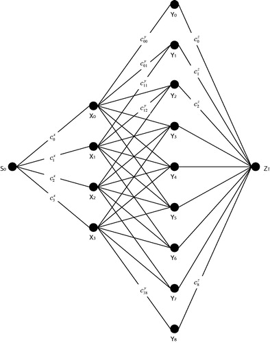
This study aims to develop an optimised chain of intervention strategies under differential inflation. This section develops a nested DP optimisation model. To explain the model, first a downscaled version of maintain, renovate, and replace optimisation problem is used in the figures and tables. Hereafter, the model formulation is applied to the full-scaled case study. In the downscaled example, the maximum technical lives for maintain, renovate, and replace options are restricted to 3, 5, and 4 years, respectively in comparison to 15, 30, and 90 years, respectively in the case study. The technical lives for the downscaled example do not have a physical meaning and are only meant for explaining the structure of the model. The total time horizon in the downscaled example is restricted to 10 years instead of an approximated infinite time horizon in the case study. Replacements (but neither cash flows nor economic lives) are considered to be repeated until the end of the time horizon as motivated in Section 3.1. The renovation option is the potential first or second intervention strategy before the replacement chain. The model allows for inclusion of more in-between intervention strategies by following the same approach.

The network corresponding to this example is visualised in Figure 1. The node $S_0$ represents the source node from which the current decisions start, and $Z_T$ represents the termination node where all replacement decisions end. The nodes $X_i$ and $Y_j$ represent the years in which maintain and renovate options end, respectively. For example, $X_3$ is read as the year in which a maintain strategy ends (here year 3) and $Y_5$ is defined as the year in which a renovation strategy ends (here year 5). The maintenance strategy starts with an existing asset in place. The path $S_0-X_3-Y_5$ therefore represents the scenario: maintain from year 0 until year 3, renovate at year 3 and keep until year 5 (two years of a renovation strategy). From year 5 onwards, the (renovated) assets will be continuously replaced over its time-variant optimised economic life. Note that in Figure 1, there are no arcs from $X_i$ to $Y_j$ for $j\mathrm{}<\mathrm{}i$ and $j\mathrm{}>\mathrm{}i\mathrm{}+\mathrm{}5$, where 5 is the maximum number of years the asset can be renovated in this example.

Figure 1. Illustrative and comprised decision network for the pumping station case study with maximum service lives for the maintain, renovate, and replacement options of respectively 3, 5 and 4 years and termination at year 10.

A decision variable $x_i$ is introduced to indicate whether the asset is maintained from year 0 till year$\mathrm{}i$. This corresponds to the arc from node $S_0$ to node $X_i$. The parameter $c_i^x$represents the present value of the corresponding cost and $N_x$ represents the maximum service life of the option to maintain. Similarly, $y_{ij}$ is introduced to indicate whether the asset is renovated from year $i$ till year $j$. This corresponds to the arc from node $X_i$ to node $Y_j$ in the network.

Again, $c_{ij}^y$ represents the present value of the corresponding cost and $N_y$ represents the maximum service life of the renovate option. Finally, decision variable $z_j$ indicates whether continuous replacements start in year $j$. This corresponds to ending the renovation of the asset in year $j$. The present value of the costs of continuous replacements from year $j$ till year $T$ (termination node $Z_T$) is denoted by $c_j^z$. The value for $c_j^z$ is obtained by solving a separate regeneration model, which is explained at the end of this section. An overview of the present values of the costs of the arcs in Figure 1 is shown in Table 2. It is emphasised that the cost variables in Table 2 represent the present values of life cycle costs from instalment until the time where a successive intervention strategy starts.

Table 2. Present values of costs of the arcs of the decision network in Figure 1.

	j	0	1	2	3	4	5	6	7	8
i	Nodes	Y0	Y1	Y2	Y3	Y4	Y5	Y6	Y7	Y8	S0
0	X0	$c_{00}^y$	$c_{01}^y$	$c_{02}^y$	$c_{03}^y$	$c_{04}^y$	$c_{05}^y$				$c_0^x$
1	X1		$c_{11}^y$	$c_{12}^y$	$c_{13}^y$	$c_{14}^y$	$c_{15}^y$	$c_{16}^y$			$c_1^x$
2	X2			$c_{22}^y$	$c_{23}^y$	$c_{24}^y$	$c_{25}^y$	$c_{26}^y$	$c_{27}^y$		$c_2^x$
3	X3				$c_{33}^y$	$c_{34}^y$	$c_{35}^y$	$c_{36}^y$	$c_{37}^y$	$c_{38}^y$	$c_3^x$
	ZT	$c_0^z$	$c_1^z$	$c_2^z$	$c_3^z$	$c_4^z$	$c_5^z$	$c_6^z$	$c_7^z$	$c_8^z$

The optimal maintain, renovate, and replace decision is given by the shortest path in this network. The shortest path in a network can be efficiently found by means of Dijkstra’s algorithm (Dijkstra, 1959). However, owing to the special structure of the network, where each path between $S_0$ and $Z_T$ has a fixed length, a more efficient backward recursion can be used, as shown in the sequence in Equation (4)(4) $$c_j^z=\underset{k=j+1,\mathrm{}\dots j+N_z}{\min }{(c}_{ji}^z+c_i^z).$$(4) . Even though the problem is not solved using LP, the LP formulation helps to understand the structure of the problem. The objective of the model is to find the least cost route from $S_0$ to $Z_T$ and is given by: (3) $$\min \left[\sum _{i=0}^{N_x}{c}_i^x\cdot x_i+\sum _{i=0}^{N_x}\sum _{j=i}^{i+N_y}{c}_{ij}^y\cdot y_{ij}+\sum _{j=0}^{N_x+N_y}{c}_j^z\cdot z_j\right]$$(3)

subject to the following constraints: $$\sum _{i=0}^{N_x}{x}_i=1,$$

$$\sum _{j=i}^{i+N_y}{y}_{ij}=x_i\forall i,$$$$\sum _{i=j-N_y}^j{y}_{ij}=z_j\forall j,$$$$x_i,y_{ij},z_j\in \left\{0,1\right\}\forall i,j.$$

3.2.1. Regeneration model

The next step is to find the cost of continuous replacements from year $j$ till year $T$, which is denoted by $c_j^z$. These continuous replacements follow from their own optimisation model, which is schematised in Figure 2 for a restricted maximum service life of a replacement option of 4 years ($N_z$ = 4 years) and a restricted time horizon of $T=10$years. To solve the optimisation of the continuous replacements, the regeneration model explained by Wagner (1975) is expanded and solved for each start year$\mathrm{}j\mathrm{}$of the possible series of replacements.

Figure 2. Schematic representation of the regeneration network for the continuous replacements.

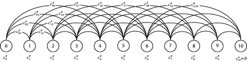
The decision variable $z_{ij}\mathrm{}$is defined to indicate whether the asset is replaced in year$\mathrm{}i$ and discarded in year$\mathrm{}j$. The present values of the corresponding costs are denoted by $c_{ij}^z$_. This is again a shortest path problem that can be solved by Dijkstra’s algorithm. Considering the case study, a more efficient DP algorithm is chosen that uses the following backward recursion: (4) $$c_j^z=\underset{k=j+1,\mathrm{}\dots j+N_z}{\min }{(c}_{ji}^z+c_i^z).$$(4)

in which, $c_{ij}^z$ is given as an input, $c_i^z$ comes from the previous iterations of the algorithm, and $N_z$ represents the maximum technical life. The recursion is initiated with $c_T^z=0$.

Similarly, the LP formulation of the problem is also provided, in which the objective function of an optimised replacement chain between year $S$ and year$\mathrm{}T\mathrm{}$is: (5) $$\min \sum _{i=S}^{T-1}\sum _{j=i+1}^T{c}_{ij}^z\cdot z_{ij}$$(5)

subject to the following constraints: $$\sum _{i=S}^{T-1}{z}_{iS}-\sum _{k=S+1}^T{z}_{Sk}=-1,$$

$$\sum _{i=S}^{T-1}{z}_{ij}-\sum _{k=S+1}^T{z}_{jk}=0\hspace{1em}\forall j\ne S,j\ne T,$$$$\sum _{i=S}^{T-1}{z}_{iT}-\sum _{k=S+1}^T{z}_{Tk}=1,$$$$z_{ij}\in \left\{0,1\right\}\hspace{1em}\forall i,j.$$

For the regeneration model, DP is preferable to LP as one run of the DP algorithm directly calculates the least costs from each start node S to termination node Z. When solving the problem for $c_0^z$, the values $c_j^z$ for all $j\mathrm{}$are found as part of the recursion. Therefore, the solutions to all regeneration models that follow the end of a renovation option are automatically found. In contrast, an LP approach to find the minimal cost $c_j^z$ would require solving 45 LP problems in the case study, one for each $j$. The costs of the arcs in Figure 2 are presented in a matrix structure in Table 3.

Table 3. Cost matrix for the regeneration model (continuous replacements, comprised example).

	j	0	1	2	3	4	5	6	7	8	9	10
i	Nodes	Z0	Z1	Z2	Z3	Z4	Z5	Z6	Z7	Z8	Z9	Z10
0	Z0		$c_{01}^z$	$c_{02}^z$	$c_{03}^z$	$c_{04}^z$
1	Z1			$c_{12}^z$	$c_{13}^z$	$c_{14}^z$	$c_{15}^z$
2	Z2				$c_{23}^z$	$c_{24}^z$	$c_{25}^z$	$c_{26}^z$
3	Z3					$c_{34}^z$	$c_{35}^z$	$c_{36}^z$	$c_{37}^z$
4	Z4						$c_{45}^z$	$c_{46}^z$	$c_{47}^z$	$c_{48}^z$
5	Z5							$c_{56}^z$	$c_{57}^z$	$c_{58}^z$	$c_{58}^z$
6	Z6								$c_{67}^z$	$c_{68}^z$	$c_{69}^z$	$c_{6,10}^z$
7	Z7									$c_{78}^z$	$c_{79}^z$	$c_{7,10}^z$
8	Z8										$c_{89}^z$	$c_{8,10}^z$
9	Z9											$c_{9,10}^z$
10	Z10

In theory, the decisions to be made on continuous replacements are infinite. In the case study, the solution space is reduced by choosing a finite boundary for $T\mathrm{}$that approximates infinity, such that cash flows beyond $T$ do not significantly contribute to the total present value of a maintain, renovate, and replacement chain. As long as the discount rate exceeds the total escalation rate of cash flows, the total present value is a concave and asymptotic function.

Several studies investigated how to assess a minimum approximation of infinity, such as Bean, Lohmann, and Smith (1994); Regnier et al. (2004); and Wagner (1975). These studies demonstrate that a minimum approximation of infinity is reached for a horizon length (terminal state) that is independent of the first decision to be made. To find such a minimum horizon length, successive approximations can be used. A DP algorithm is terminated as soon as an additional time period does not influence the first decision.

As a practical and safe estimate for public infrastructure assets with high investment costs and relatively low O&M expenditures, a boundary of 300 years is chosen as an approximation of infinity. The motivation is that the real costs of a full replacement in year 300 contribute to only a factor $1/{\left(1+i_{\mathit{\text{real}}}\right)}^n=1/(1+0.05{)}^{300}=4.4·10^{-7}$ to the total present value of all costs between year 0 and year 300. Three hundred years is in line with another case study dealing with capital-intensive infrastructure with long service lives (coastal flood protection) presented by Brekelmans et al. (2012); Zwaneveld and Verweij (2014); and Dupuits et al. (2017).

3.3. Present value calculations under inflation and age-related cost increases

This section outlines the calculation of the present values $c_i^x,\mathrm{}{c}_{ij}^y$, and $c_{ij}^z$ ($c_j^z$ follows from the application of the regeneration model). The variable $c_i^x$ represents the present value of maintaining the pumping station from year 0 to year $i$, $c_{ij}^y$ represents the present value of a renovate option that starts in year $i$ and ends in year $j$, and $c_{ij}^z$ represents the present value of a replace option that starts in year $i$ and ends in year $j$.

The cost calculations under total inflation, differential inflation, and age-related cost increases are rarely addressed in the literature. These factors are a real issue in practice. The relations between total inflation $f_{tot}$, differential inflation $f_d$, general inflation $f_g$, real interest rate $i_{\mathit{\text{real}}}$, and nominal interest rate $i_{nom}$ are depicted in Equations (1)(1) $$i_{nom}=i_{\mathit{\text{real}}}+f_g+i_{\mathit{\text{real}}}\cdot f_g=(1+i_{\mathit{\text{real}}})(1+f_g)-1,$$(1) and (2)(2) $$f_{tot}=f_g+f_d+f_g\cdot f_d=(1+f_g)\cdot (1+f_d)-1.$$(2) . The general inflation rate is equal for all cost categories: investments, major overhauls, O&M expenditures, and electricity costs. The differential inflation differs across categories, and therefore the total inflation rate is also specific for a cost category.

Inflation should be treated consistently in present value analyses. Equations (1) and (2) define: Cash flows that are inflated with the total inflation rate $f_{tot}$ are discounted with the nominal or effective discount rate $i_{nom}$. Cash flows that are inflated with a differential inflation rate $f_d$ are discounted with the real interest rate $i_{\mathit{\text{real}}}\mathrm{}$(Brealey et al., 2017; Park, 2011; Sullivan et al., 2012): (6) $$\frac{(1+f_{tot})}{(1+i_{nom})}=\frac{(1+f_g)(1+f_d)}{(1+i_{nom})}=\frac{(1+f_d)}{{(1+i_{\mathit{\text{real}}})}^{}}$$(6)

Discounting of real and nominal cash flows with the appropriate discount rate leads to the same present values, as noted in Equations (1)(1) $$i_{nom}=i_{\mathit{\text{real}}}+f_g+i_{\mathit{\text{real}}}\cdot f_g=(1+i_{\mathit{\text{real}}})(1+f_g)-1,$$(1) and (2)(2) $$f_{tot}=f_g+f_d+f_g\cdot f_d=(1+f_g)\cdot (1+f_d)-1.$$(2) . By definition, all present values $c_i^x,\mathrm{}{c}_{ij}^y$, and $c_{ij}^z$have the same baseline $t=0$. The following equations are used to calculate the present values. The equations are expressed in nominal terms, and their symbols and indices are presented in Table 4.

Table 4. Symbols and indices used in present value equations.

$t$	Time of purchase or instalment ($t=0$ for $c_i^x\mathrm{}and\mathrm{}t=i$ for $c_{ij}^y$ , $c_{ij}^z$)
$I$	Initial investment cost
$S$	Salvage value
$D$	Demolition costs
$H$	Costs of a major overhaul
$M$	First year’s operation and maintenance costs
$E$	First year’s electricity costs
${\mathrm{}}_I$	Index for investment
${\mathrm{}}_S$	Index for salvage values
${\mathrm{}}_D$	Index for demolition costs
${\mathrm{}}_H$	Index for major overhauls
${\mathrm{}}_M$	Index for operation and maintenance costs
${\mathrm{}}_E$	Index for electricity costs
${\mathrm{}}_{(0)}$	Index for current price level, real (non-inflated) costs, constant currency
$f_{tot}$	Total inflation rate [% per year]
$f_g$	General inflation rate [% per year]
$f_d$	Differential inflation rate [% per year]
$i_{nom}$	Nominal interest rate [% per year]; includes general inflation
$i_{\mathit{\text{real}}}$	Real interest rate [% per year]; excludes general inflation
$g$	Age related price increase [% per year]
$b$	Reduction of the initial investment for calculating the salvage value [% per year]
$dm$	A percentage of the initial investment to calculate the end of life demolition costs [%]
$n$	The age of an asset when disposed of ($n=i$ for $c_i^x\mathrm{}and\mathrm{}n=j$ for $c_{ij}^y$ , $c_{ij}^z$)
${n_1,\mathrm{}{n}_2,\mathrm{}..\mathrm{}n}_q$	The age at which the 1^st, 2^nd, … q^th major overhaul takes place with $n_q<n$
$P$	The present value (t = 0) of cash flows incurred from $t$ to $t+n$

Under differential inflation, the present value ($t=0$) of an initial investment $I$ for an asset bought in year $t$ and disposed of at age $n$ is modelled as: (7) $$P_{I[t,t+n]}=\frac{I_{\left(0\right)}{(1+f_g)}^t{(1+f_{d,I})}^t}{{(1+i_{nom})}^t}.$$(7)

The initial investment expressed in the current price level for an asset bought in year $t$ is inflated with general inflation and differential inflation to year $t$, and discounted with the nominal discount rate from year $t$ to the present.

Public infrastructure assets generally do not have salvage values from trading as motivated in Section 3.1. However, if these salvage values are relevant, the present value of a salvage value of an asset bought in year $t$ and disposed of at age $n$ can be modelled as: (8) $$P_{S[t,t+n]}=\frac{-I_{\left(0\right)}{(1+f_g)}^t{(1+f_{d,I})}^t\cdot {(1-b)}^n{(1+f_g)}^n{(1+f_{d,S})}^n}{{(1+i_{nom})}^{t+n}}.$$(8)

The factor $b$ represents an annual reduction in the initial investment, expressed as a percentage. The investment is first inflated to the year of purchase, then reduced to calculate the salvage value at age $n$. A minus sign is added before the investment costs as a salvage value is income. The salvage value may have different inflation rates than the initial investment, and therefore the salvage value is inflated from year $t$ to age $n$ with its own inflation rate. Finally, the inflated salvage value at time $t+n$ is discounted to the present using the nominal discount rate.

In the case of end-of-life time-variant demolition costs $D$, the present value of these costs can be modelled in a similar manner, as shown in Equation (9)(9) $$P_{D[t,t+n]}=\frac{I_{\left(0\right)}{(1+f_g)}^t{(1+f_{d,I})}^t\cdot dm\cdot {(1+f_g)}^n{(1+f_{d,D})}^n}{{(1+i_{nom})}^{t+n}}$$(9) . The time-variant demolition costs are modelled as a percentage $dm$ of the initial investment at age $n$ and a separate inflation rate for the demolition costs is used: (9) $$P_{D[t,t+n]}=\frac{I_{\left(0\right)}{(1+f_g)}^t{(1+f_{d,I})}^t\cdot dm\cdot {(1+f_g)}^n{(1+f_{d,D})}^n}{{(1+i_{nom})}^{t+n}}$$(9)

However, for the infrastructure case study, demolition costs are not considered to be age-related (no significant age-related scrap value) and included as fixed costs in the successive investment costs.

Major overhauls ($H_{\left(0\right),1},\mathrm{}{H}_{\left(0\right),2},\mathrm{}\dots ,\mathrm{}{H}_{\left(0\right),q}$) are planned periodically at age ${n_1,n_2,\mathrm{}\dots ,\mathrm{}n}_q$, while $H_{\left(0\right),1}$ is the cost of the first major overhaul in the current price level, $H_{\left(0\right),2}\mathrm{}$is the cost of the second major overhaul in the current price level, and $H_{\left(0\right),q}\mathrm{}$is the cost of the last major overhaul in the current price level. The parameter $n_q$ represents the age of the asset at the last major overhaul, a number of years before the end of its service life ($n$). The present value of major overhauls of an asset bought at time $t$ and disposed of at age $n$ is modelled as follows: (10) $$\begin{array}{c}{P}_{H[t,t+n]}=\frac{H_{\left(0\right),1}{(1+f_g)}^{t+n_1}{(1+f_{d,H_1})}^{t+n_1}}{{(1+i_{nom})}^{t+n_1}}\\ +\frac{H_{\left(0\right),2}{(1+f_g)}^{t+n_2}{(1+f_{d,H_2})}^{t+n_2}}{{(1+i_{nom})}^{t+n_2}}\\ +\dots +\frac{H_{\left(0\right),q}{(1+f_g)}^{t+n_q}{(1+f_{d,H_q})}^{t+n_q}}{{(1+i_{nom})}^{t+n_q}}.\end{array}$$(10)

The yearly O&M expenditures ($M$) can be subject to both inflation and age-related price increases ($g$). O&M expenditures can increase with age owing to increasing failures and maintenance needs. To model the present value of O&M expenditures, the geometric gradient factor is adapted by substituting $i_{nom}\mathrm{}$for $i_{\mathit{\text{real}}}$, conforming to Equation (1)(1) $$i_{nom}=i_{\mathit{\text{real}}}+f_g+i_{\mathit{\text{real}}}\cdot f_g=(1+i_{\mathit{\text{real}}})(1+f_g)-1,$$(1) .

The generic geometric gradient with cash flows in real terms is (Newnan et al., 2016; Park, 2011; Sullivan et al., 2012): (11) $$P_{}=A_{1,\mathit{\text{real}}}\frac{1-{(1+p)}^n{(1+i_{\mathit{\text{real}}})}^n}{i_{\mathit{\text{real}}}-p}.$$(11)

where parameter A₁ is the first year’s real costs, $n$ is the age of the asset, and $p$ is an annual percentage price increase. First, $p$ is split into a part reflecting differential inflation and a part reflecting age-related price increases as follows: $$\begin{array}{c}(1+p)=(1+f_d)(1+g)\Rightarrow \\ p=(1+f_d)(1+g)-1.\end{array}$$

Substituting $(1+p)$ and $p$ in Equation (11)(11) $$P_{}=A_{1,\mathit{\text{real}}}\frac{1-{(1+p)}^n{(1+i_{\mathit{\text{real}}})}^n}{i_{\mathit{\text{real}}}-p}.$$(11) results in: (12) $$P_{}=A_{1,\mathit{\text{real}}}\frac{1-{(1+f_d)}^n{(1+g)}^n{(1+i_{\mathit{\text{real}}})}^{-n}}{i_{\mathit{\text{real}}}-(1+f_d)(1+g)+1}$$(12)

Expressing the right-hand side in nominal terms requires the substitution of: $$(1+i_{\mathit{\text{real}}})=\frac{(1+i_{nom})}{(1+f_g)}$$

$$i_{\mathit{\text{real}}}=\frac{(i_{nom}-f_g)}{(1+f_g)}$$$$A_{1,\mathit{\text{real}}}=\frac{A_{1,nom}}{{(1+f_g)}^1}$$

Performing these substitutions results in a geometric gradient with cash flows expressed in nominal terms as follows: (13) $$P_{}=A_{1,nom}\frac{1-{(1+f_d)}^n{(1+g)}^n{(1+f_g)}^n{(1+i_{nom})}^{-n}}{i_{nom}-(1+f_d)(1+g)(1+f_g)+1}$$(13)

Using this expression, the present value of O&M expenditures for an asset bought at time $t$and kept in service for $n$ years is modelled as: (14) $$P_{M[t,t+n]}=\frac{M_{\left(0\right)}{(1+f_g)}^{t+1}{(1+f_{d,M})}^{t+1}{(1+g_M)}^1}{{(1+i_{nom})}^t}\cdot \frac{1-{(1+f_g)}^n{(1+f_{d,M})}^n{(1+g_M)}^n{(1+i_{nom})}^{-n}}{i_{nom}-(1+f_g)(1+f_{d,M})(1+g_M)+1}.$$(14)

The parameter $M_{(0)}$ represents the first-year O&M costs in the current price level (base year 0), which are inflated from year 0 to the first year after purchase $(t+1)$ of an asset. These inflated first year O&M costs are then multiplied with the classic geometric gradient factor, adapted for nominal cash flows. This results in the nominal future value of a series of $n$ years of increasing O&M costs at the time of purchase $t$. To find the present value (base year 0), these costs are discounted over $t$ using the nominal discount rate.

A similar process is followed to calculate the present value of the annual electricity costs $E$: (15) $$P_{E[t,t+n]}=\frac{E_{\left(0\right)}{(1+f_g)}^{t+1}{(1+f_{d,E})}^{t+1}{(1+g_E)}^1}{{(1+i_{nom})}^t}\cdot \frac{1-{(1+f_g)}^n{(1+f_{d,E})}^n{(1+g_E)}^n{(1+i_{nom})}^{-n}}{i_{nom}-(1+f_g)(1+f_{d,E})(1+g_E)+1}.$$(15)

The age-related price increase for electricity costs $g_E$ could arise, for example, owing to greater electricity consumption as assets age.

Excluding salvage values from trading and time-variant demolition costs (see case study description in Section 3.1 for the underlying motivation), the total present value of an asset ($t=0$) installed in year $t$ and kept until year $t+n$ is calculated using Equations (7)(7) $$P_{I[t,t+n]}=\frac{I_{\left(0\right)}{(1+f_g)}^t{(1+f_{d,I})}^t}{{(1+i_{nom})}^t}.$$(7) , (10)(10) $$\begin{array}{c}{P}_{H[t,t+n]}=\frac{H_{\left(0\right),1}{(1+f_g)}^{t+n_1}{(1+f_{d,H_1})}^{t+n_1}}{{(1+i_{nom})}^{t+n_1}}\\ +\frac{H_{\left(0\right),2}{(1+f_g)}^{t+n_2}{(1+f_{d,H_2})}^{t+n_2}}{{(1+i_{nom})}^{t+n_2}}\\ +\dots +\frac{H_{\left(0\right),q}{(1+f_g)}^{t+n_q}{(1+f_{d,H_q})}^{t+n_q}}{{(1+i_{nom})}^{t+n_q}}.\end{array}$$(10) , (14)(14) $$P_{M[t,t+n]}=\frac{M_{\left(0\right)}{(1+f_g)}^{t+1}{(1+f_{d,M})}^{t+1}{(1+g_M)}^1}{{(1+i_{nom})}^t}\cdot \frac{1-{(1+f_g)}^n{(1+f_{d,M})}^n{(1+g_M)}^n{(1+i_{nom})}^{-n}}{i_{nom}-(1+f_g)(1+f_{d,M})(1+g_M)+1}.$$(14) , and (15)(15) $$P_{E[t,t+n]}=\frac{E_{\left(0\right)}{(1+f_g)}^{t+1}{(1+f_{d,E})}^{t+1}{(1+g_E)}^1}{{(1+i_{nom})}^t}\cdot \frac{1-{(1+f_g)}^n{(1+f_{d,E})}^n{(1+g_E)}^n{(1+i_{nom})}^{-n}}{i_{nom}-(1+f_g)(1+f_{d,E})(1+g_E)+1}.$$(15) as follows: (16) $$c_{[t,t+n]}=P_{I[t,t+n]}+P_{H[t,t+n]}+P_{M[t,t+n]}+P_{E[t,t+n]}.$$(16)

Equation (16)(16) $$c_{[t,t+n]}=P_{I[t,t+n]}+P_{H[t,t+n]}+P_{M[t,t+n]}+P_{E[t,t+n]}.$$(16) is used to calculate the present values $c_i^x,c_{ij}^y$, and $c_{ij}^z$. Regarding the formulation of the shortest path problems in Section 3.2, the following is considered: $$t=0\text{for}{c}_i^x,$$ $$t=i\text{for}{c}_{ij}^y,c_{ij}^z,$$ $$n=i\text{for}{c}_i^x,$$ $$n=j\text{for}{c}_{ij}^y,c_{ij}^z.$$

3.4. Results of the optimised maintain, renovate, and replacement chain for the case study

The present values $c_i^x,\mathrm{}{c}_{ij}^y$, and $c_{ij}^z$ for the case study are obtained using Equation (16)(16) $$c_{[t,t+n]}=P_{I[t,t+n]}+P_{H[t,t+n]}+P_{M[t,t+n]}+P_{E[t,t+n]}.$$(16) . The DP recursion in Equation (4)(4) $$c_j^z=\underset{k=j+1,\mathrm{}\dots j+N_z}{\min }{(c}_{ji}^z+c_i^z).$$(4) is first used to calculate the $c_j^z$ values of the regeneration model (Figure 2), which in the current case study represent the present values of a chain of optimised continuous replacements starting at $t\mathrm{}=\mathrm{}0,\mathrm{}1,\mathrm{}2,\mathrm{}\dots ,\mathrm{}45$ and ending at $T_Z=300$years. Hereafter, the combined maintain, renovate, and continuously replace network is solved (Figure 1) using the same DP recursion. The Java code for the nested implementation of this backward recursion is given in Appendix A. The results of the regeneration model for continuous replacements that start at $t\mathrm{}=\mathrm{}0\mathrm{}$are presented in Table 5. The $c_j^z$ values for $j$ = 0–45 (thus, the total present values of each optimal replacement chain starting at time j) are shown in Figure 3.

Table 5. Results of optimised continuous replacements when starting at t = 0.

Regeneration model starting at t = 0	Replace	Replace	Replace	Replace	Replace
Optimal life	60	60	60	60	60
Time interval	[0,60]	[60,120]	[120,180]	[180, 240]	[240, 300]
Present values (baseline t = 0)	$c_{\mathrm{0,60}}^z$ = € 3,237,632	$c_{\mathrm{60,120}\mathrm{}}^z$= € 547,643	$c_{\mathrm{120,180}}^z$ = € 93,695	$c_{\mathrm{180,240}}^z$ = € 16,152	$c_{\mathrm{240,300}}^z=$€ 2,798
Total present value	$c_{0\mathrm{}}^z$= € 3,897,920

Figure 3. Present values $c_j^z$ of optimised replacement chains starting at t = j and ending at t = 300.

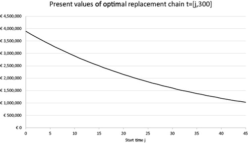
The current case study uses DP to calculate the future optimal service lives of the continuous replacements starting at $t\mathrm{}=\mathrm{}0\mathrm{}$and ending at t = 45. The postponement of this optimised replacement chain will decrease its present value as depicted in Figure 3. These present values ${(c}_j^Z)\mathrm{}$in Figure 3 represent the optimised cost values for the final paths $Y_j-Z_t$ in Figure 1. Table 5 illustrates that the economic lives of future challengers remain unchanged from the current viewpoint. This is a characteristic of the current case study. Different asset types with different cost profiles will result in other economic lives which are not likely to be equal. In addition, starting the replacement chain in the future instead of $t\mathrm{}=\mathrm{}0\mathrm{}$influences economic lives. Although economic service lives of the continuous replacements are similar in the current case study, it still needs a DP solution for continuous replacements as differential inflation rejects the repeatability assumption of the future cash flows. A comparison with a classic approach (without DP solutions) follows in Section 3.5.

The combined optimisation model in Figure 1 incorporates the current defender with the renovation option and continuous replacements. In essence, solving the mathematical model does not differ from the regeneration model. The only difference is another network structure, a different corresponding cost matrix, and different cost values. The final calculation results are presented in Table 6. The optimal strategy is to replace the pumping station immediately. The optimised path is $X_0$, $Y_0$, and $Z_{300}$ (recall that the index represents the year in which the activity ends). Several additional infrastructure case studies with other realistic input data were considered in this DP model leading to different paths for optimal strategies, such as path $X_{15}$, $Y_{25}$, and $Z_{300}$. The path $X_0$, $Y_0$, and $Z_{300}$ of the current case study may not appear very exciting. However, this path is an equally optimised path among many possible paths.

Table 6. Results of optimised maintain, renovate, and replacement chain.

Maintain, renovate, replace	Maintain	Renovate	Replace and regenerate
Node	X0	Y0	Z300
Service life	0 years	0 years	300 years
Time	[0,0]	[0,0]	[0,300]
Present values (base line t = 0)	$c_0^x$= € 0	$c_{\mathrm{0,0}}^y$ = € 0	$c_0^z$= € 3,897,920
Total present value	P[0,300] = € 3,897,920

3.5. Comparison of the classic approach to replacement analysis

The classic approach to replacement analysis compares the minimum Equivalent Annual Cost (EAC*) values of maintain, renovate, and replace options at their economic lives. The classic theory is well described in textbooks by authors such as Blank and Tarquin (2012); Hastings (2015); Newnan et al. (2016); Park (2011); and Sullivan et al. (2012).

As explained in Section 2, the classic economic life comparison cannot be used when differential inflation is involved. A decision maker not familiar with DP techniques could therefore choose to ignore differential inflation or to include differential inflation in the classic calculation techniques. Both situations are incorrect. In the first case, the calculations are correct but real costs caused by differential inflation are ignored. In the second case, there is an attempt to include real costs caused by differential inflation, but the calculations will be incorrect owing to the repeatability assumption of the challengers’ cash flows that will not hold in the comparison of EAC* values. Both cases are investigated and compared to the optimal DP solution.

Excluding differential inflation in the case study (all differential inflation is set to zero), results in the EAC* values as depicted in the top part of Table 7. Based on these values, a decision maker would maintain the defender for 5 years. The major overhaul necessary for maintaining the defender at the end of year 5 prompts a renovation. The renovated pumping station is retained for 30 years before replacing it. The classic approach in this example searches for the least total present value which is obtained by the lowest sequence of EAC* values as the expensive major overhauls will enforce an intervention at the calculated economic lives. Without major overhauls, optimised intervention times in a classic defender-challenger replacement analysis may occur a couple of years beyond the economic service lives (Park, 2011). Nevertheless, this is not the case in the current case study.

Table 7. Classic EAC* comparison calculated at t = 0.

Baseline t = 0	EAC*	n* (years)
Excluding differential inflation
Maintain now and keep for 5 years	€ 121,822	5
Renovate now and keep for 30 years	€ 129,703	30
Replace now and keep for 60 years	€ 138,430	60
Including differential inflation
Maintain now and keep for 5 years	€ 123,765	5
Renovate now and keep for 10 years	€ 136,496	30
Replace now and keep for 60 years	€ 143,109	60

The total present value of this scenario is presented in Table 8 and follows from straightforward discounting of a 5 years’ annuity of €121,822 starting in year 1, a 30 years’ annuity of €129,703 starting in year 6, and an infinite annuity of €138,430 starting in year 36. Note that annuities start 1 year after an investment, thus, in year $t+1$ and are first discounted to year t. Hereafter, this local present value is discounted to the present to$\mathrm{}t\mathrm{}=\mathrm{}0$.

Table 8. Comparison of DP solution and classic replacement techniques.

Intervention strategies	Maintain	Renovate	Replace and regenerate	Total present value
Classic without differential inflation	5 years t = [0,5]	30 years t = [5,35]	Infinite t = [35, ∞]	€ 3,262,784
Classic with differential inflation (wrong application)	5 years t = [0,5]	30 years t = [5,35]	Infinite t = [35, ∞]	€ 3,397,622
Optimal DP solution	0 years	0 years	Infinite t = [0, approx. ∞]	€ 3,897,920

The second case includes differential inflation in the classic economic life comparison. This leads to the EAC* values depicted in the bottom part of Table 7. The EAC* values are marginally higher owing to extra costs induced by differential inflation. Based on these EAC* values, a decision maker would also maintain the pumping station for 5 years, renovate and retain it for 30 before replacing it. This is not correct as the EAC* values should not be treated as constants, as a consequence of differential inflation. The total present value is presented in Table 8 and calculated similar to the previous case, though only the cost values differ.

Comparing the classic approach with the DP model shows a difference in optimal strategies and in their total present values. The classic approach underestimates the total cost of the case study in a range of k€500 to k€635 on an investment volume of k€2,500 in comparison to the optimal DP solution. Under estimating the real costs leads to a suboptimal strategy. The DP solution favours an early replacement, while the classic approach advises to postpone the replacement because the relative high differential inflation on O&M expenditures make the maintenance and renovate options less attractive.

Under differential inflation and multiple successive intervention strategies, it is not possible to derive generic rules that estimate the deviations from the classic approach as too many variables are involved. Therefore, each case study needs to be judged on its case-specific circumstances. The number of successive intervention strategies is of importance. The cost profiles of intervention strategies may differ significantly. Differential inflation is positive in the case study considered, but it can also be negative depending on the type of costs considered. As ageing plays a role, the timing of major overhauls can be a decisive factor. Discount rates are important too. Low discount rates, as seen in public sector organisations, amplify the impact of differential inflation. The current study demonstrates that differential inflation matters and requires careful assessment.

The contribution of the current research to existing literature is twofold. First, for infrastructure assets, it confirms the case-specific conclusion of other authors on the limitations of classic replacement techniques. Second, the current research developed a novel nested DP model capable of dealing with multiple successive intervention strategies under differential inflation. Instead of three intervention strategies in the case study (maintain, renovate, and continuously replace), more intervention strategies can be included, following the same approach.

4. Discussion and limitations

Although DP and LP techniques provide accurate results in comparison to classic replacement techniques, there are limitations to this approach. In all likelihood, the most important one is that practitioners are not familiar with DP and LP techniques. Replacement analyses using these techniques are not found in conventional textbooks on engineering economics. Applying this approach in practice may therefore be challenging.

A second limitation to the nested DP model is its deterministic nature. This does not undermine the value of the described optimisation method. Probabilistic models are used to incorporate uncertainty in the timing and size of costs. These probabilistic models underlie the cost values in the cost matrices. Adding a probabilistic model would improve the accuracy of the cost matrices and results of the approach, but would not alter the nested optimisation method. The challenge of introducing uncertainty in the current optimisation approach is considered for further research.

A third limitation to the case study is that only two challengers are considered, a renovation option and a continuously replace option. The future may hold more than two challengers. Adding additional challengers to the described optimisation approach follows the same methodology, but will require more cost calculations of the paths in the network. This study proposes to be practical. The case study shows that for the cash flow patterns of common public infrastructure assets, decisions generally occur before one of the major overhauls or the end of the technical life of an asset. This is owing to the fact that major overhauls are expensive, and the costs of overhauls are generally much greater than the regular O&M expenditures. Cost calculation efforts can be significantly reduced by limiting the decision nodes to the intervals of the major overhauls and technical lives. This will also enhance the applicability of the model in practice.

A fourth limitation is that the future is uncertain. Nevertheless, the prime interests of a maintenance engineer are the short- and mid-term decisions, which are influenced by the long-term estimates of future costs. A reasonable estimate of the future costs is adequate in this context. The described optimisation approach already provides a more accurate estimate than the classic methods, which assume continuous repeatability of the first challenger’s life cycle cash flows. Finally, emphasis should be given to the complexity of replacement decisions in general and least costs are just one of the replacement criteria involved.

5. Conclusions

Several authors have investigated the application of classic replacement techniques under inflation and technological change, and concluded in their case studies that using classic replacement techniques will lead to errors. DP and LP techniques are required to identify optimal replacement strategies when the assumption of continuous repeatability of life cycle cash flows of future intervention strategies does not hold. Case-specific modelling is applied to find the least cost route in a network of probable future scenarios.

In this study, a novel nested DP model is developed for a replacement problem that is common for many public-sector infrastructure organisations. This replacement problem is demonstrated in a case study that consists of an existing asset and multiple successive intervention strategies under differential inflation. The multiple intervention strategies include a renovate option followed by a continuously replace option as a final estimate for future cash flows.

Although the last intervention strategy considers continuous replacements, the life cycle cash flows of these replacements are non-repeatable owing to differential inflation. The optimisation model can be extended with more successive intervention strategies which allows for simulating flexible technology change. Total inflation, differential inflation, and age-related cost increases are explicitly addressed as these are realistic in practice and should not be ignored. The optimisation model is applied to a case-study which demonstrates that the inclusion of differential inflation influences the optimised total intervention strategy.

The entire optimisation model is described as a nested DP approach. First, the continuously replace optimisation is solved, providing the present values of replacement chains starting at different future times. Second, the three alternatives (maintain, renovate, and continuously replace) are combined and optimised for the lowest total present value. This yields an optimal intervention chain for maintaining, renovating, and replacing the asset.

For infrastructure assets, optimal intervention decisions are very likely to occur just before a major overhaul or the end of the technical life of an asset. This feature can be used to reduce the size of the solution matrix and cost calculations. The optimisation approach provides a realistic solution for a common infrastructure asset replacement problem of an existing asset and multiple successive intervention strategies under differential inflation.

Appendix A

Java code nested DP recursion

W[_nYearsTotal] = 0;

for (intk = _nYearsTotal-1; k> = 0; k--) {

doublebestValue = Double.MAX_VALUE;

intbestOption = -1;

for (intl = k + 1; l< = Integer.min(_nYearsTotal, l + 90); l++) {

doublevalue = _costReplace[k][l] + W[l];

if (value < bestValue) {

bestValue = value;

bestOption = l;

}

}

W[k] = bestValue;

WChoice[k] = bestOption;

}

for(intj = 0; j< = _nYearsMaintain; j++) {

doublebestValue = Double.MAX_VALUE;

intbestOption = -1;

for (intl = j; l< = j + 30; l++) {

doublevalue = _costRenovate[j][l] + W[l];

if (value < bestValue) {

bestValue = value;

bestOption = l;

}

}

Y[j] = bestValue;

YChoice[j] = bestOption;

}

doublebestValue = Double.MAX_VALUE;

intbestOption = -1;

for(inti = 0; i< = _nYearsMaintain; i++) {

doublevalue = _costMaintain[i] + Y[i];

if (value < bestValue) {

bestValue = value;

bestOption = i;

}

}

X = bestValue;

XChoice = bestOption;

References

- Adey, B. T., Burkhalter, M., & Lethanh, N. (2018). Determining an optimal set of work zones on large infrastructure networks in a GIS framework. Journal of Infrastructure Systems, 24(1), 04017048.
- Bean, J. C., Lohmann, J. R., & Smith, R. L. (1994). Equipment replacement under technological change. Naval Research Logistics (NRL), 41(1), 117–128.
- Bellman, R. (1955). Equipment replacement policy. Journal of the Society for Industrial and Applied Mathematics, 3(3), 133–136.
- Blank, L. T., & Tarquin, A. J. (2012). Engineering economy. New York: McGraw-Hill Education.
- Bocchini, P., & Frangopol, D. M. (2011). A probabilistic computational framework for bridge network optimal maintenance scheduling. Reliability Engineering and System Safety, 96(2), 332–349.
- Brealey, R. E., Myers, S. C., & Allen, F. (2017). Principles of corporate finance (4th ed.). New York: McGraw-Hill Education.
- Brekelmans, R. C. M., den Hertog, D., Roos, C., & Eijgenraam, C. (2012). Safe dike heights at minimal costs: The nonhomogeneous case. Operations Research, 60(6), 1342–1355.
- Büyüktahtakın, İE., & Hartman, J. C. (2016). A mixed-integer programming approach to the parallel replacement problem under technological change. International Journal of Production Research, 54(3), 680–695.
- Campbell, J. D., Jardine, A. K. S., & McGlynn, J. (2011). Asset management excellence: optimizing equipment life-cycle decisions. Boca Raton, FL: CRC Press.
- Christer, A. H., & Goodbody, W. (1980). Equipment replacement in an unsteady economy. The Journal of the Operational Research Society, 31(6), 497–506.
- Christer, A. H., & Scarf, P. A. (1994). A robust replacement model with applications to medical equipment. The Journal of the Operational Research Society, 45(3), 261–275.
- Dijkstra, E. W. (1959). A note on two problems in connexion with graphs. Numerische Mathematik, 1(1), 269–271.
- Dupuits, E. J. C., Schweckendiek, T., & Kok, M. (2017). Economic optimization of coastal flood defense systems. Reliability Engineering and System Safety, 159, 143–152.
- Frangopol, D. M., Kallen, M.-J., & Noortwijk, J. M V. (2004). Probabilistic models for life-cycle performance of deteriorating structures: review and future directions. Progress in Structural Engineering and Materials, 6(4), 197–212.
- Frangopol, D. M. F. A., Estes, A. C. M. A., & Stewart, M. G. M. A. (2004). Bridge deck replacement for minimum expected cost under multiple reliability constraints. Journal of Structural Engineering, 130(9), 1414–1419.
- Gertsbakh, I. (2000). Reliability theory with applications to preventive maintenance: Springer-Verlag.
- Golabi, K., Kulkarni, R. B., & Way, G. B. (1982). A statewide pavement management system. Interfaces, 12(6), 5–21.
- Hartman, J. C. (2004). Multiple asset replacement analysis under variable utilization and stochastic demand. European Journal of Operational Research, 159(1), 145–165.
- Hartman, J. C., & Murphy, A. (2006). Finite-horizon equipment replacement analysis. IIE Transactions, 38(5), 409–419. doi: 10.1080/07408170500380054
- Hastings, N. A. J. (2015). Physical Asset Management. London, New York: Springer.
- Hillier, F. S., & Lieberman, G. J. (2010). Introduction to operations research (9th ed.). Boston, MA: McGraw-Hill.
- Jardine, A. K. S., & Tsang, A. H. C. (2013). Maintenance, replacement and reliability. New York: CRC Press.
- Karsak, E. E., & Tolga, E. (1998). An overhaul-replacement model for equipment subject to technological change in an inflation-prone economy. International Journal of Production Economics, 56–57, 291–301. doi: 10.1016/j.ejor.2010.09.011
- Mardin, F., & Arai, T. (2012). Capital equipment replacement under technological change. The Engineering Economist, 57(2), 119.
- de Neufville, R., Scholtes, S., & Wang, T. (2006). Real options by spreadsheet: Parking garage case example. Journal of Infrastructure Systems, 12(2), 107–111.
- Newnan, D. G., Lavelle, J. P., & Eschenbach, T. G. (2016). Engineering economy analysis. New York: Oxford University Press.
- Oakford, R. V., Lohmann, J. R., & Salazar, A. (1984). A dynamic replacement economy decision model. IIE Transactions, 16(1), 65.
- Park, C. S. (2011). Contemporary engineering economics (15th ed.). New Jerssey: Pearson.
- Regnier, E. V. A., Sharp, G., & Tovey, C. (2004). Replacement under ongoing technological progress. IIE Transactions, 36(6), 497–508.
- Scarf, P. A., & Hashem, M. H. (1997). On the Application of an economic life model with a fixed planning horizon. International Transactions in Operational Research, 4(2), 139–150.
- Sullivan, W. G., Wicks, E. M., & Koeling, C. P. (2012). Engineering economy. Boston: Pearson, Prentice Hall.
- Wagner, H. M. (1975). Principles of operations research: with applications to managerial decisions (2nd ed.). London: Prentice-Hall.
- Yatsenko, Y., & Hritonenko, N. (2011). Economic life replacement under improving technology. International Journal of Production Economics, 133(2), 596.
- Zwaneveld, P. J., & Verweij, G. (2014). Safe dike heights at minimal costs - An integer programming approach. CPB Netherlands Bureau for Economic Policy Analysis, Den Haag. Retrieved from https://www.cpb.nl/sites/default/files/publicaties/download/cpb-discussion-paper-277-safe-dike-heights-minimal-costs-integer-programming-approach.pdf.