A Stochastic View on the Effect of Random Rail Irregularities on Railway Bridge Vibrations

Abstract

This contribution studies dynamic amplification factors that consider the impact of random rail irregularities on the deflection and acceleration response of simple railway bridges. Response statistics for a set of plane fully coupled bridge–vehicle interaction models with random irregularity profiles are derived by Monte Carlo simulations. The underlying samples of random irregularity profiles are generated from a power spectral density function, assuming that the uneven rail surface is governed by a Gaussian stochastic process in space. A modified bootstrap method is used to identify the required sample size of profiles for sufficiently accurate description of the random response. On the basis of this pilot study, a parametric response examination of short span railway bridges with variable length, fundamental frequency, structural mass and damping, and track quality in a range commonly observed in real structures is conducted. A statistical representation of the uncertain bridge response is employed for analytical modelling of the response amplification due to random rail irregularities considering limit state-based exceedance probabilities. The results are compared to outcomes of existing simplified approaches in design codes used to take into account the effect of rail irregularities on the dynamic bridge response, showing the improvement of the developed framework.

Keywords:

• Bridge dynamics
• high-speed train
• random rail irregularity
• bootstrap method
• Monte Carlo simulation

1. Introduction

Rail irregularities are defined as small imperfections of the rail track profile from its idealised geometry. They comprise the surface unevenness between rail and train wheels as well as deviations of the three-dimensional (3D) track curve from its designed state. In general, it is distinguished between isolated rail irregularities caused by rail joints and local sleeper settlements, and random rail irregularities. Sources of the latter type are wear, clearances, subsidence, insufficient maintenance of the permanent rail track or railway bridge structures, etc. (Frýba, 1996), and implicate misalignment, elevation (vertical settlement), superelevation (tilting) of sleepers and twist, and gauge imperfections of the rails (Yang, Yau, & Wu, 2004).

Although the worldwide net of railway lines is permanently maintained in an effort to ensure smooth track profiles, rail irregularities cannot be completely avoided. When passed by the train, rail irregularities induce noise affecting the environment along the lines and may lead to passengers riding discomfort due to vehicle vibrations. In the worst case, they might even bear a safety risk when causing train derailment. Furthermore, in combination with the moving train, these imperfections represent a significant source of excitation of the track pavement, subsoil and civil structures such as railway bridges along the line. Having in mind that the number of high-speed lines with common traveling speeds of 55.6 m/s ($\approx 200$ km/h) and beyond is rapidly increasing, it is of particular importance to understand the effect of geometric deviations of the rail track on the vibration response of track pavement and rail network structures. In further consequence, applicable tools need to be developed that allow to consider this influence in the design phase of these structures accurately.

The interaction of the train vehicle with the uneven rail track has been studied extensively in the literature, see, e.g., Lei & Noda (2002) or Nielsen & Igeland (1995), or the more recent work of Colaço, Costa, and Connolly (2016). In contrast, very few studies are focusing on the prediction of the dynamic railway bridge response in the presence of random rail irregularities. The monographs (Frýba, 1996; Yang et al., 2004) provide an overview how different kinds of rail irregularities can be implemented in a numerical model, and they also show for a few selected bridge objects the predicted dynamic response. In some case studies, such as in Antolín et al. (2013) and Malveiro, Sousa, Ribeiro, and Calcada (2018), the interaction between bridge structure, train and irregular rail surfaces is investigated. These contributions examine only the effect of a single irregular profile representation, which matches measured random rail track geometry data, on the bridge and train response. In another paper, Majka and Hartnett (2009) derive a dynamic impact factor for bridge deflection and compute the bridge deck and vehicle acceleration response considering the effect of rail irregularities for different track quality classes and different train types. The outcomes of this study are also based on a single random profile each for lateral, vertical left and right rail geometry. For instance, it is found that the influence of the irregularity profile on the vertical dynamic amplification factor is minor. However, such single rail profile representations cannot capture the random nature of the dynamic bridge and train response.

In a more elaborate stochastic approach, Au, Wang, and Cheung (2002) analyse random samples of a cable stayed bridge, using up to 20 different realisations of rail profiles. In particular, mean value and standard deviation of an impact factor for the bridge deflection are derived. According to this study, only ten different profiles provide the basis for a sufficient statistical displacement representation. A more recent contribution (Cantero, Arvidsson, OBrien, & Karoumi, 2016) investigates the scatter of the wheel–rail force and the bridge accelerations in the presence of rail irregularities using 15 profiles. Arvidsson, Andersson, and Karoumi (2019) employ a sample size of 24 rail irregularity realisations, also focusing on the response scatter and the wheel–rail contact interaction. An alternative stochastic approach to direct simulation is presented by Yu, Mao, Guo, and Guo (2016), where a probability density evolution method is applied to evaluate response statistics of a railway bridge with random rail imperfections. As a reference solution serve the outcomes of a Monte Carlo simulation with large samples of 5000 random profiles.

Large samples of random irregularity profiles are also used for the reliability analysis of railway bridges (e.g. Rocha, Henriques, & Calcada, 2016; Salcher, Pradlwarter, and Adam 2016), where, among other outcomes, it was found that the bridge acceleration is considerably affected by rail imperfections, depending on the power spectral density function describing the rail roughness. As it has been shown, for instance, in Cantero et al. (2016) and Kuisle (2018), irregularities with short wavelengths ($\lambda \le 25$ m) have the largest impact on the dynamic bridge deflection and acceleration as well as on the wheel–rail interaction force. While the Eurocode EN13848-5 (2010) regulates the maximum allowed irregularity amplitudes dependent on the wavelength to maintain running safety and track quality, no specifications of such amplitudes for numerical response simulations are provided in European guidelines so far.

For railway bridge design in engineering practice, dynamic computations based on moving single force models are state of the art to predict the dynamic bridge response (see, e.g., EN1991-2, 2003; Johansson, Nualláin, Pacoste, & Andersson 2014). For serviceability limit states (SLSs), the maximum bridge deflections and the bridge accelerations must be kept small to provide passenger riding comfort, to prevent ballast destabilisation and to minimise the risk of derailment (EN1990, 2013). Moving single force load models do not allow to directly account for track irregularities, because bridge–vehicle interaction is not considered. Hence, in the design code EN1991-2 (2003), the response amplification due to irregular rail surfaces is captured simplified through the following amplification factor $\phi ″,$ (1) $$\phi ″=\frac{\alpha }{100}[56e^{-{(L/10)}^2}+50(\frac{L{f}_g}{80}-1\left)e^{-{(L/20)}^2}\right] , \alpha =\min \{v/22,1\}$$(1) where L is the span in the case of a simply supported bridge, f_g is the first natural bending bridge frequency and v is the actual train speed. Factor ${\phi }^{″}$ applies for standard maintained tracks. For carefully maintained tracks, such as high-speed railway lines, the amplification factor can be reduced by 50% (i.e. ${\phi }^{″}/2$) (see EN1991-2, 2003). All bridge response quantities of dynamic computations based on perfect rails (such as internal forces, deflections, accelerations) must be amplified by the same factor ${\chi }^{(\mathit{AUT})}=1+\phi ″/2$ (see for instance the national provision in Austria (ÖBB-RLI-Dynamik, 2011)). According to Gulvanessian, Formichi, Calgaro, and Harding (2009), factor ${\phi }^{″}$ is based on a single vertical rail pump of 2 mm over 1 m in length and 6 mm vertical over 3 m in length, respectively, passed by an unsprung wheel mass of 2000 kg. It should be noted that ${\phi }^{″}$ (respectively ${\phi }^{″}/2$) is supposed to represent an upper bound of bridge amplification due to geometric rail imperfections. However, in many cases the response predicted by elaborated numerical simulations is larger than the response amplified by $\phi ″$ (Gulvanessian et al., 2009).

In contrast to most previous investigations, this article does not study the effect of a single irregularity profile on bridge vibrations, but aims at capturing the statistical dynamic response of simple bridge structures with rather short span due to random rail imperfections. Therefore, it is necessary to access the required number of different irregular rail profiles to obtain a representative stochastic response description of both bridge deflection and acceleration response in the context of a Monte Carlo simulation. A further objective of this study is to derive an improved dynamic response amplification factor based on random irregular rail profiles.

The present article is organised as follows. After a brief description of the utilised bridge–vehicle interaction model, the mathematical representation of random rail irregularities is discussed. Then, the response scatter resulting from a Monte Carlo simulation on a case study object provides the basis to derive statistics and distributions of the dynamic peak bridge deflection and acceleration. A bootstrap method delivers the sample size required for a reliable response description. Based on this sample size, subsequently a parametric study capturing a wide range of simply supported railway bridges with different span, fundamental frequency, mass, damping and track quality is conducted. The outcomes of this study are used to derive novel response amplification factors, which describe more realistically the effect of rail irregularities on the dynamic bridge response. Finally, the proposed amplification factors are set in contrast to the counterparts implemented in a design code, and the differences are discussed in detail.

2. Bridge–vehicle interaction model

2.1 General strategy

Commonly, the numerical prediction of the dynamic response of railway bridges subjected to high-speed trains is based on a series of single forces crossing the bridge with a certain train speed v (see, e.g., EN1991-2, 2003; Johansson et al., 2014; Moyo & Tait, 2010). Each of these single forces represents a static axle load of a generic train or a real train. Such simplified approach does not capture the actual interaction between bridge and train, and consequently, the impact of rail irregularities on the dynamic system response cannot be directly predicted.

Since a primary goal of this study is to quantify the dynamic response amplification due to imperfect rails, the simplest possible general model that explicitly accounts for dynamic interaction between bridge and train vehicle is employed. In this model, a Euler–Bernoulli beam represents the bridge structure, and the train is described by a planar mass–spring–damper (MSD) system. In a component mode synthesis (CMS) method according to Biondi, Muscolino, and Sofi (2005), the equations of motion of the bridge structure and the train model are derived separately and subsequently coupled by imposing the compatibility conditions at the interface of both subsystems.

In a numerical bridge–vehicle model, rail irregularities are commonly represented by generalised irregularity rail profiles that are superimposed to the smooth track (bridge) axis. At the contact point, the wheel is, thus, subjected to a base excitation composed of profile irregularity and bridge deflection. The utilised modelling strategy captures all essential characteristics of dynamic bridge–vehicle interaction with lowest possible numerical effort and, thus, allows for a comprehensive parametric study to quantify the effect of rail irregularities with reasonable expense.

2.2 Euler–Bernoulli beam bridge

The considered simply supported continuous Euler–Bernoulli beam bridge model of span L is depicted in Figure 1. This model accounts for load-bearing structure, ballast, sleepers and rails. Lateral beam deflection $w_b(x,t)$ of the undamped Euler–Bernoulli beam bridge with uniform bending stiffness EI and mass per unit length ρA subjected to a series of N_w concentrated forces $F_b^{(i)}(t),i=1,\dots ,N_w,$ moving with constant speed v is governed by the following partial differential equation of motion (Adam & Salcher, 2014; Yang et al., 2004), (2) $$\rho A{\ddot{w}}_b(x,t)+\mathit{EI}{w}_{b,\mathit{xxxx}}(x,t)=\sum _{i=1}^{N_w}{F}_b^{\left(i\right)}\left(t\right)\delta (x-{\xi }_i)\left(H\right(t-t_i^{\left(0\right)})-H(t-t_i^{\left(E\right)}\left)\right)$$(2)

Figure 1. Simply supported Euler–Bernoulli beam bridge subjected to interface forces. Modified from Salcher and Adam (2018).

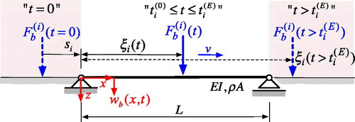
Position ${\xi }_i=\mathit{vt}-s_i$ of the ith interaction force $F_b^{(i)}(t)$ between track and the ith wheel pair of the train at time t is indicated by delta function $\delta (x-{\xi }_i)$ (see Figure 1). Heaviside functions H control the arrival and departure, respectively, of $F_b^{(i)}$ on the beam model at instant times $t_i^{(0)}=s_i/v$ and $t_i^{(E)}=(s_i+L)/v,$ respectively. Modal expansion of $w_b(x,t)$ by considering only the first $N_{\varphi }$ eigenfunctions ${\varphi }_n(x),w_b(x,t)\approx {\sum }_{n=1}^{N_{\varphi }}{\varphi }_n(x)q_n(t),$ decouples the partial differential equation of motion into $N_{\varphi }$ ordinary single degree-of-freedom oscillator equations in terms of modal coordinates $q_n(t)$ (Ziegler, 1998), (3) $$\begin{array}{l}{\ddot{q}}_n\left(t\right)+2{\zeta }_n{\omega }_n{\dot{q}}_n\left(t\right)+{{\omega }_n}^2{q}_n\left(t\right)=p_n\left(t\right), p_n\left(t\right)=\sum _{i=1}^{N_w}{F}_b^{\left(i\right)}\left(t\right){\varphi }_n(x={\xi }_i)\left(H\right(t-t_i^{\left(0\right)})-H(t-t_i^{\left(E\right)}),\\ & {\omega }_n={\left(\frac{n\pi }{L}\right)}^2\sqrt{\frac{\mathit{EI}}{\rho A}}, {\varphi }_n=\hspace{0.17em}\text{sin}\hspace{0.17em}\frac{n\pi x}{L},m_n=\frac{\rho \mathit{AL}}{2}, n=1,\dots ,N_{\varphi }\end{array}$$(3) where bridge damping ζ_n has been added modally. In a common assumption, the damping coefficient of each mode is assumed to be the same, that is ${\zeta }_n=\zeta ,n=1,\dots ,N_{\varphi }.$ The $N_{\varphi }$ modal equations of motion condensed written in matrix form, (4) $${\mathbf{M}}_b\ddot{\mathbf{q}}+{\mathbf{C}}_b\stackrel{\mathbf{̇}}{\mathbf{q}}+{\mathbf{K}}_b\mathbf{q}={\mathbf{P}}_b$$(4)

represent the mechanical model of the bridge subsystem. Herein, ${\mathbf{M}}_b,{\mathbf{C}}_b,{\mathbf{K}}_b,{\mathbf{P}}_b$ denote the modal mass matrix, modal damping matrix, modal stiffness matrix and modal interaction force vector, respectively, (5) $$\begin{array}{ll}\hfill & {\mathbf{M}}_b=\text{diag}[m_1,\dots ,m_{N_{\varphi }}] , {\mathbf{C}}_b=\text{diag}[2{\zeta }_1{m}_1{\omega }_1,\dots ,2{\zeta }_{N_{\varphi }}{m}_{N_{\varphi }}{\omega }_{N_{\varphi }}] , \hfill \\ \hfill & {\mathbf{K}}_b=\text{diag}[m_1{\omega }_1^2,\dots ,m_{N_{\varphi }}{\omega }_{N_{\varphi }}^2] , {\mathbf{P}}_b={[p_1,\dots ,p_{N_{\varphi }}]}^T\hfill \end{array}$$(5) and $\mathbf{q}={[q_1,\dots ,q_{N_{\varphi }}]}^T.$

The Euler–Bernoulli beam bridge model is fully characterised by its span L, fundamental bending frequency $f_g={\omega }_1/(2\pi ),$ total mass $\rho \mathit{AL}$ and damping coefficient ζ. In the subsequent parametric study, f_g and $\rho \mathit{AL}$ are selected from the railway bridge catalogue compiled in Doménech, Museros, and Martínez-Rodrigo (2014). In Figure 2, the parameter range defined in this railway bridge catalogue is highlighted by grey shaded areas. To the left, the frequency range for common high-speed railway bridges according to EN1991-2 (2003) is shown as a function of span L for short spans up to L = 30.0 m, with lower and upper frequency boundaries $f_g^{(1)}$ (min EC) and $f_g^{(5)}$ (max EC), respectively. To the right, upper and lower bounds of the total bridge mass in this span range are plotted. This mass range is treated to be independent from the bridge fundamental frequency (Doménech et al., 2014). Note that Figure 2 depicts additional information for the subsequent convergence and parameter study (diamond and triangle markers, additional lines $f_g^{(2-4)}$) discussed in sections 3.3 and 4.1. Damping coefficient ζ is employed according to the span-dependent relations defined in EN1991-2 (2003) for steel (${\zeta }_{D1}$), prestressed concrete (${\zeta }_{D2}$) and concrete bridges (${\zeta }_{D3}$) (see Table 1). For the purposes of the present study, the dynamic response is sufficiently accurately approximated by $N_{\varphi }=5$ modes, verified in preliminary convergence studies (see also Salcher, 2015).

Figure 2. (a) Fundamental frequency and (b) mass range considered in the present study according to the bridge catalogue of Doménech et al. (2014).

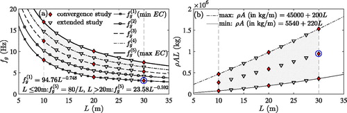
Table 1. Damping values according to EN1991–2 (2003).

	Lower limit of damping value ζ in %
Bridge type	Span L < 20 m	Span $L\ge 20$ m
${\zeta }_{D1}:$ Steel and composite	$\zeta =0.5+0.125(20-L)$	$\zeta =0.5$
${\zeta }_{D2}:$ Prestressed concrete	$\zeta =1.0+0.07(20-L)$	$\zeta =1.0$
${\zeta }_{D3}:$ Filler beam and reinforced concrete	$\zeta =1.5+0.07(20-L)$	$\zeta =1.5$

2.3 Vehicle model

The vehicles of the train subsystem are modelled as planar mass–spring–damper (MSD) systems, consisting of rigid bodies with mass, which represent passenger stage, two bogies and four wheel pairs, connected by spring-dashpot elements. As such, the interaction between bridge and vehicle can be considered and, consequently, also the effect of rail irregularities. Figure 3 shows the MSD system, representing both the power car and passenger cars of the Austrian high-speed train type Railjet, used in this study as reference high-speed train. In total, this vehicle model exhibits ten degrees-of-freedom (DOFs), that is seven translational DOFs and three rotational DOFs (see Figure 3). Detailed geometry, mass, stiffness and damping parameters are specified in ÖBB-RLI-Dynamik (2011) and Salcher (2015).

Figure 3. Planar MSD model for the jth vehicle of the high-speed train Railjet, modified from Salcher and Adam (2015).

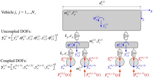
The equation of motion of the jth car read as (Salcher & Adam, 2015): (6) $${\mathbf{M}}_v^{\left(j\right)}{ÿ}^{\left(j\right)}\left(t\right)+{\mathbf{C}}_v^{\left(j\right)}{\stackrel{.}{\mathbf{y}}}^{\left(j\right)}\left(t\right)+{\mathbf{K}}_v^{\left(j\right)}{\mathbf{y}}^{\left(j\right)}\left(t\right)={\mathbf{f}}_v^{\left(j\right)}\left(t\right) , j=1,\dots ,N_v$$(6) where displacement vector ${\mathbf{y}}^{(j)}(t)={[{\mathbf{y}}_0^{(j)}(t),{\mathbf{y}}_w^{(j)}(t)]}^{\mathrm{T}}$ is split into subvector ${\mathbf{y}}_0^{(j)}$ containing the six DOFs of passenger stage and boogies, and subvector ${\mathbf{y}}_w^{(j)}$ containing the four DOFs of the four wheels in contact with the bridge surface. Excitation vector ${\mathbf{f}}_v^{(j)}(t)$ is composed of the static axle loads $S_w^{(i)}$ and wheel contact forces $F_w^{(i)}(t)$ at the interface of the ith wheel to the bridge surface (compare with Figure 3). A detailed description of the involved subsystem matrices and vectors is found in Salcher and Adam (2015). The model train is composed of N_v = 8 vehicles (a power car and seven passenger cars) assumed to be kinematic decoupled from each other with total N_w = 32 axles.

2.4 Subsystem coupling

The equations of motion of the beam and MSD subsystems, Equation (4)(4) $${\mathbf{M}}_b\ddot{\mathbf{q}}+{\mathbf{C}}_b\stackrel{\mathbf{̇}}{\mathbf{q}}+{\mathbf{K}}_b\mathbf{q}={\mathbf{P}}_b$$(4) and Equation (6)(6) $${\mathbf{M}}_v^{\left(j\right)}{ÿ}^{\left(j\right)}\left(t\right)+{\mathbf{C}}_v^{\left(j\right)}{\stackrel{.}{\mathbf{y}}}^{\left(j\right)}\left(t\right)+{\mathbf{K}}_v^{\left(j\right)}{\mathbf{y}}^{\left(j\right)}\left(t\right)={\mathbf{f}}_v^{\left(j\right)}\left(t\right) , j=1,\dots ,N_v$$(6) , respectively, are coupled according to the so-called corresponding assumption (see Zhang, Xia, Guo, & De Roeck, 2010). This assumption implies that the elasticity of wheel and track at the contact point is neglected and a continuous contact of the bodies is supposed. That is, lift-off of the wheels is not admitted. Consequently, the vertical displacement of the ith wheel pair, $y_w^{(i)}(t),$ corresponds to the rail deflection at contact point ${\xi }_i(t),$ which is composed of bridge deflection $w_b({\xi }_i(t),t)$ and rail irregularity described by profile function $I_r({\xi }_i(t))$ (Salcher & Adam, 2015; Zhang et al., 2010), (7) $$y_w^{\left(i\right)}\left(t\right)=w_b\left({\xi }_i\right(t),t)+I_r\left({\xi }_i\right(t\left)\right)\approx \sum _{n=1}^{N_{\varphi }}{\varphi }_n\left({\xi }_i\right(t\left)\right)q_n\left(t\right)+I_r\left({\xi }_i\right(t\left)\right), i=1,\dots ,N_w(=4N_v)$$(7)

Accordingly, the contact force between each wheel pair and track is equal, $F_w^{(i)}=F_b^{(i)},i=1,\dots ,N_w.$ The coupled system is governed by the following system of differential equations (8) $$\overline{\mathbf{M}}\stackrel{..}{\overline{\mathbf{y}}}+\overline{\mathbf{C}}\stackrel{.}{\overline{\mathbf{y}}}+\overline{\mathbf{K}}\overline{\mathbf{y}}=\overline{\mathbf{f}}$$(8) where $\overline{\mathbf{y}}={[\mathbf{q},{\mathbf{y}}_0^{(1)},{\mathbf{y}}_0^{(2)},\dots ,{\mathbf{y}}_0^{(N_v)}]}^{\mathrm{T}}$ contains only the modal coordinates of the beam and the internal DOFs ${\mathbf{y}}_0^{(j)}$ of each vehicle, $1\le j\le N_v.$ Matrices $\overline{\mathbf{M}},\overline{\mathbf{C}}$ and $\overline{\mathbf{K}}$ are time dependent due to coupling condition Equation (7)(7) $$y_w^{\left(i\right)}\left(t\right)=w_b\left({\xi }_i\right(t),t)+I_r\left({\xi }_i\right(t\left)\right)\approx \sum _{n=1}^{N_{\varphi }}{\varphi }_n\left({\xi }_i\right(t\left)\right)q_n\left(t\right)+I_r\left({\xi }_i\right(t\left)\right), i=1,\dots ,N_w(=4N_v)$$(7) . Vector $\overline{\mathbf{f}}$ contains the modal representation of the static axle loads, and first- and second-order time derivatives of irregularity profile functions $I_r({\xi }_i(t))$ evaluated at position ${\xi }_i(t).$ For further details of the applied CMS approach, the involved system matrices and vectors, it is referred to Biondi et al. (2005), Salcher (2015) and Salcher and Adam (2015).

A Newmark-β algorithm is used to solve the coupled system of equations (Equation 8(8) $$\overline{\mathbf{M}}\stackrel{..}{\overline{\mathbf{y}}}+\overline{\mathbf{C}}\stackrel{.}{\overline{\mathbf{y}}}+\overline{\mathbf{K}}\overline{\mathbf{y}}=\overline{\mathbf{f}}$$(8) ) for modal coordinates $q_1,\dots ,q_{N_{\varphi }}$ collected in vector q and their second time derivatives. Substituting these quantities into the modal series expansion of $w_b(x,t)$ and ${\ddot{w}}_b(x,t),$ respectively, yields the response of the bridge at time instant t and any position x along the beam axis. In combination with a sufficiently small time step, the Newmark integration method is unconditionally stable.

It is important to point out that this simplified planar interaction model should only be used for beam-like bridge structures, because a planar model cannot account for torsional and horizontal vibration effects present in more irregular structures. For instance, in Salcher (2015), it was shown that the response prediction based on a beam model and on a more elaborated 3D finite element model of a regular beam-like bridge is very similar if the first bending natural frequencies of both models coincide. The simplified modelling approach utilised in the present study has been frequently used in recent research, in particular for numerically expensive investigations, as for instance in Xia, Zhang, and Guo (2006) and Doménech et al. (2014).

2.5 Random rail irregularity profiles

The non-smooth profile line representing rail irregularities is considered to be entirely random and modelled as a stochastic Gaussian ergodic process in space (Frýba, 1996). Since the length of a bridge is finite (and often short), the statistical response quantities cannot be computed from a bridge–train model with one specific irregular rail profile, but should be evaluated from the response of various model samples each with a different profile realisation. Consequently, a set of random rail profiles must be generated.

In the present planar model representation, according to Claus and Schiehlen (1998), each of the random and likewise planar (vertical) rail irregularity profiles $I_r(x)$ at an arbitrary position x along the track (with $0\le x\le \infty$) is described by its spatial mean value $\overline{I_r}$ and its autocorrelation function $R_{I_r},$ (9) $$\overline{I_r}=\underset{Y\to \infty }{\lim }\frac{1}{Y}{\int }_0^Y{I}_r\left(x\right)\mathrm{d}x , R_{I_r}\left(\xi \right)=\underset{Y\to \infty }{\lim }\frac{1}{Y}{\int }_0^Y{I}_r\left(x\right)I_r(x-\xi )\mathrm{d}x$$(9)

Application of a Fourier transformation yields the single sided power–spectral–density (PSD) function $S(\Omega ),\Omega \ge 0,$ for the profile functions, (10) $$S\left(\Omega \right)=2{\int }_{-\infty }^{\infty }{R}_{I_r}\left(\xi \right)e^{-i\Omega \xi }\mathrm{d}\xi$$(10) which characterises the rail irregularities as a function of the spatial circular frequency $\Omega =2\pi /\lambda$ with wavelength λ. To classify the track quality, national authorities (including China, France, Germany and US) provide different closed form irregularity PSD functions, which have been fitted to the outcomes of measurements (see Cantero et al., 2016; Frýba, 1996).

For the present study, the vertical PSD used in Germany (Claus & Schiehlen, 1998) (11) $$S\left(\Omega \right)=Q_r\frac{{\Omega }_c^2}{2({\Omega }_r^2+{\Omega }^2)({\Omega }_c^2+{\Omega }^2)}$$(11) with ${\Omega }_c=0.8246$ m^{− 1} and ${\Omega }_r=0.0206$ m^{− 1}, is employed. Spectral amplitude Q_r defines the roughness of the random rail profiles, ranging from $Q_{r,0}=5.923 {10}^{-7}$ m for high quality rails to $Q_{r,1}=15.861 {10}^{-7}$ m for very poor rail quality with large irregular deviations (see Claus & Schiehlen, 1998). Linear interpolation of these boundary values according to $Q_r(a)=Q_{r,0}+a(Q_{r,1}-Q_{r,0})$ with $0\le a\le 1$ yields spectral amplitudes $Q_r(a)$ that describe intermediate rail states. At the outset of numerical response simulations, random irregular rail profiles are computed based on the PSD function, Equation (11)(11) $$S\left(\Omega \right)=Q_r\frac{{\Omega }_c^2}{2({\Omega }_r^2+{\Omega }^2)({\Omega }_c^2+{\Omega }^2)}$$(11) , by the finite inverse Fourier transformation (Claus & Schiehlen, 1998) (12) $$I_r\left(x\right)=\sqrt{\frac{2}{\pi }}\sum _{j=1}^J{A}_j\hspace{0.17em}\text{cos}\hspace{0.17em}({\Omega }_{j}x+{\phi }_j) , A_j=\sqrt{S\left({\Omega }_j\right)\Delta \Omega }$$(12) where the random phase angle ${\phi }_j$ has been added, which is uniformly distributed in the range $0\le {\phi }_j\le 2\pi$ for each of the J discrete spatial frequencies Ω_j, and ${\Omega }_{j+1}={\Omega }_j+\Delta \Omega .$ The irregularity profiles of this study are generated by the superposition of J = 1000 harmonics according to Equation (12)(12) $$I_r\left(x\right)=\sqrt{\frac{2}{\pi }}\sum _{j=1}^J{A}_j\hspace{0.17em}\text{cos}\hspace{0.17em}({\Omega }_{j}x+{\phi }_j) , A_j=\sqrt{S\left({\Omega }_j\right)\Delta \Omega }$$(12) at discrete spatial frequencies evenly spaced between ${\Omega }^{(1)}=\pi /50$ m^{− 1} and ${\Omega }^{(2)}=\pi$ m^{− 1}, thus simulating wavelengths from ${\lambda }^{(2)}=2$ m to ${\lambda }^{(1)}=100$ m. The resulting profiles with zero mean exhibit standard deviations of 1.14 mm ($Q_r(a=0)$), 1.55 mm ($Q_r(a=0.5)$) and 1.87 mm ($Q_r(a=1.0)$). 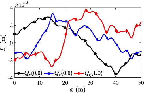As an example, Figure 4 shows three of these random irregularity profiles of 50 m length, one describing high quality ($Q_r(0),$ black), one medium quality ($Q_r(0.5),$ blue) and one poor quality ($Q_r(1.0),$ red) rails.

Figure 4. Example of three random vertical rail irregularity profiles for a track of 50 m length with good (black), medium (red) and poor rail quality (blue), respectively.

3. Quantification of the response variation

3.1 Case study for the response scatter

At first, the effect of rail irregularities on the dynamic bridge response is demonstrated on the example of a case study object. A simply supported bridge of span L = 30.0 m, total mass $\rho \mathit{AL}=9.47\times {10}^5$ kg, first natural bending frequency $f_g={\omega }_1/(2\pi )=3.15$ Hz and damping coefficient $\zeta =1\%$ subjected to the Railjet train is considered. In the parameter space depicted in Figure 2, the red diamond markers highlighted by a blue circles refer to the parameters of this object. The rail quality is assumed to be poor, that is $Q_r(a=1.0),$ when generating the arbitrary selected number of 1000 random irregularity profiles. The result of a crude Monte Carlo simulation is shown in Figure 5, where in subplot (a) the peak deflection, $w=\max |w_b(x,t)|,$ and in subplot (b) the peak acceleration, $\ddot{w}=\max |{\ddot{w}}_b(x,t)|,$ of the 1000 bridge samples is plotted in grey dotted lines against train speed v.

Figure 5. (a) Peak deflection and (b) peak acceleration of an example bridge with span 30.0 m. 1000 bridge samples with random irregularity profiles describing poor rail quality. Statistical response quantities. Reference solution: bridge with perfect rails.

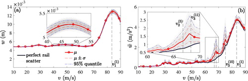
Note that these response quantities represent the peak values both with respect to the location x along the bridge span (i.e. not necessarily at midspan) and time t. Such spectral response representation provides a global overview of the response scatter for varying train speeds v, but the information of time instant t and location x of the peak response is lost. Additionally, mean μ (red solid lines with circular markers), mean μ ± standard deviation σ (red dashed lines) and 95% quantile (blue dashed-dotted lines) of these peak response quantities are depicted. A full black line refers to the outcomes of the reference bridge without rail irregularities (i.e. the rail surface is perfectly smooth). The peak acceleration $\ddot{w}$ does not necessarily occur at midspan, because higher modes contribute significantly to this response quantity. For instance, in the studies of Rocha, Henriques, and Calçada (2014) and Salcher and Adam (2015) for most train speeds, the peak bridge acceleration was found either at the quarter spans or at 2/3 of the span. Cantero and Karoumi (2016) report similar findings for the bridge acceleration and conclude that the higher modes are excited by higher excitation frequencies from the axle spacing or local irregularity frequencies. This effect is, however, commonly negligible for the deflection response (Cantero & Karoumi, 2016). As observed in Figure 5, both the spectral maximum displacement and maximum acceleration exhibit a distinct peak at resonance speed $v_1^{(1)}=83.5$ m/s. In general, resonance speed $v_n^{(m)}=f_n{d}_v/m$ corresponds to the mth resonance of the nth mode due to the train excitation (Xia et al., 2006), with the regular car length $d_v=26.5$ m for the Railjet model, and neglects changes in the bridges natural frequencies due to interaction effects (Cantero, Hester, & Brownjohn, 2017).

While in the speed range $0\le v\le 70$ m/s the maximum bridge displacement is smooth without significant dynamic amplification, the acceleration exhibits some peaks at various resonance speeds less than $v_1^{(1)},$ in particular if rail irregularities are taken into account. It is also observed that for this case study object mean peak deflection of the uneven bridge and the corresponding reference solution of the structure with perfect rails are almost identical. However, the peak acceleration of most samples exceeds the corresponding reference acceleration, thus yielding a mean acceleration response considerably larger than the acceleration of the bridge without rail imperfections. Dispersion, and thus also the standard deviation, of the bridge deflection is almost constant at speeds larger than 25 m/s. On the contrary, dispersion of the peak acceleration is more pronounced and also tends to become larger with increasing train speed and is particularly pronounced at some resonance speeds, for instance at $v_3^{(10)}=75.1$ m/s and $v_3^{(11)}=68.3$ m/s. Note that the latter speed related to the third mode is close to $v_2^{(5)}=66.8$ m/s, where the second bridge mode is excited to resonance.

3.2 Modified bootstrapping method

The outcomes of the Monte Carlo simulation on this case study object represent a response pool, because the underlying sample size of 1000 is much larger than necessary to fully capture the response statistics. However, it is of foremost interest to choose the minimum number of discrete irregularity profiles that allows for an accurate numerical prediction of the response statistics of bridge–train systems, that is mean value μ and standard deviation σ of bridge deflection w and bridge acceleration $\ddot{w}.$ To identify this required sample size of irregularity profiles, in the following a modified bootstrapping approach (see Davison & Hinkley, 1997) is applied. In contrast to basic bootstrapping by Efron (1979), where each bootstrap sample size is identical to the original sample size N₀, sample size N_l of the resampled data (bridge response) is variable but always $N_l\le N_0.$

The procedure is as follows. For the considered bridge parameter combination, the response for an initial sample of size N₀ at a chosen speed V is computed, yielding a set $\mathbf{x}={\left\{x^{(i)}\right\}}_{i=1}^{N_0}$ of N₀ representations of the peak deflection ($x^{(i)}=w^{(i)}(v=V)$) and peak acceleration ($x^{(i)}={\ddot{w}}^{(i)}(v=V)$), respectively. From this source set x, a total number of K independent new bootstrap samples ${\tilde{\mathbf{x}}}_k$ ($1\le k\le K$) are drawn with replacement, with the size of these resamples $N_l\le N_0.$ To each source realisation $x^{(i)},$ the same discrete probability $p_i=1/N_0$ is assigned. Then, from each bootstrap sample ${\tilde{\mathbf{x}}}_k={\left\{{\tilde{x}}_k^{(i)}\right\}}_{i=1}^{N_l},$ the kth statistics, that is mean μ_k and standard deviation σ_k, are computed, (13) $${\mu }_k=\frac{1}{N_l}\sum _{i=1}^{N_l}{\tilde{x}}_k^{\left(i\right)}$$(13) (14) $${\sigma }_k^2=\frac{1}{N_l-1}\sum _{i=1}^{N_l}({\tilde{x}}_k^{\left(i\right)}-{\mu }_k{)}^2$$(14)

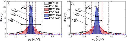
As an example, for the peak acceleration at speed V = 68.0 m/s of the case bridge object from above, Figure 6 visualises these statistics for three distinctive resample sizes, $N_l=\{20,100,1000(=N_0)\},$ and a bootstrap range of K = 5000 repetitions. The considered speed V corresponds to resonance speed $v_3^{(11)},$ highlighted in Figure 5(b). Figure 6(a) shows histograms (denoted as HIST), which represent an approximation of the distribution of the mean response $\ddot{w}(V)$ based on N_l = 20 (grey), 100 (red) and 1000 (blue), respectively, irregularity profiles. In Figure 6, additionally probability density functions (PDF) of Gaussian distributions fitted to the bootstrap results are plotted, which are subsequently used to estimate confidence intervals of the outcomes. Since the standard deviations of $\ddot{w}(V)$ depicted in Figure 6(b) show the same localisation tendency as the mean, the distributions of the kth statistics can be used to estimate the minimum sample size of random irregular track profiles for reliable Monte Carlo simulations.

Figure 6. Histogram and corresponding fitted Gaussian density functions for (a) mean and (b) standard deviation of the peak acceleration of the case study bridge at V = 68 m/s. Bootstrap resample sizes of 20, 100 and 1000 irregularity profiles.

To quantify the observed localisation effect, in a next step means ${\mu }_{N_l}^{(\mu )},{\mu }_{N_l}^{(\sigma )}$ and standard deviations ${\sigma }_{N_l}^{(\mu )},{\sigma }_{N_l}^{(\sigma )}$ of the kth statistics of the resamples of size N_l are computed, (15) $${\mu }_{N_l}^{\left(\mu \right)}=\frac{1}{K}\sum _{k=1}^K{\mu }_k , {\mu }_{N_l}^{\left(\sigma \right)}=\frac{1}{K}\sum _{k=1}^K{\sigma }_k$$(15) (16) $${\sigma }_{N_l}^{(\mu )2}=\frac{1}{K-1}\sum _{k=1}^K({\mu }_k-{\mu }_{N_l}^{(\mu )}{)}^2 , {\sigma }_{N_l}^{(\sigma )2}=\frac{1}{K-1}\sum _{k=1}^K({\sigma }_k-{\mu }_{N_l}^{(\sigma )}{)}^2$$(16)

Because the standard deviations of the resamples, ${\sigma }_{N_l}^{(\mu )}$ and ${\sigma }_{N_l}^{(\sigma )},$ decrease with increasing number N_l of considered irregularities profiles, as observed in Figure 6, this quantity can be used as convergence criterion of the spectral response statistics.

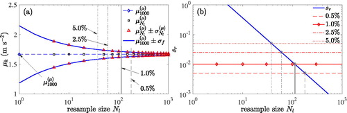
Figure 7(a) illustrates for the mean μ_k of the peak acceleration (at speed V = 68.0 m/s) this convergence behaviour with increasing resample size N_l. Black square markers correspond to the resample mean ${\mu }_{N_l}^{(\mu )}$ at different discrete sample sizes $N_l.$ It is seen that for all considered resample sizes, the resampled mean response is almost identical with the actual mean acceleration of $\ddot{w}=1.67$ m/s², which was estimated with the largest considered sample size of $N_0=1000$ irregularity profiles and a basic bootstrap sample with K = 5000 repetitions. Additionally, the standard deviation from the mean, ${\mu }_{N_l}^{(\mu )}\pm {\sigma }_{N_l}^{(\mu )},$ is plotted by red triangle markers against discrete values of N_l, visualising the localisation tendency of the distribution. It is obvious that this quantity approaches asymptotically the mean with increasing resample size.

Figure 7. Convergence of the mean peak acceleration of the example bridge at speed V = 68 m/s with increasing resample size. (a) Discrete mean and mean ± standard deviation, and fitted function. (b) Relative slope of the fitted standard deviation with a = 0.483, $b=-0.486$ and $c=-0.002.$

To define a termination criterion, that is the sample size where convergence can be assumed, subsequently standard deviations ${\sigma }_{N_l}^{(\mu )}$ of the modified bootstrap samples are expressed by regression function σ_f of type (17) $${\sigma }_f\left(N_l\right)=a{N}_l^b+c$$(17) with parameters a, b and c fitted to match the discrete data. In particular, the relative slope of this function computed as the ratio of ${\sigma }_f^{\prime }(N_l)=\mathrm{d}{\sigma }_f/\mathrm{d}{N}_l$ at resample size N_l over slope ${\sigma }_f^{\prime }(N_l=5)$ at an initial resample size N_l = 5 serves as convergence indicator $s_r(N_l);$ $s_r(N_l)={\sigma }_f^{\prime }(N_l)/{\sigma }_f^{\prime }(5).$ That is, convergence is attained if this relative slope falls below a limit value $s_r^{(\mathit{limit})}$ to be specified. In Figure 7(b), for the peak acceleration at V = 68.0 m/s relative slope $s_r(N_l)$ of the standard deviation is plotted against resample size N_l in logarithmic scale (blue solid line). With an arbitrarily defined limit value $s_r^{(\mathit{limit})}=0.01,$ at a sample size N_l = 112, the relative slope s_r drops below 1%, and the mean response subsequently is considered as converged. Returning to Figure 7(a), the statistical quantities read at N_l = 112 provide an overview of the response scatter related to this sample size limit. For this example, the choice of $s_r^{(\mathit{limit})}=1\%$ corresponds to the 95% confidence interval of the mean acceleration, $\ddot{w}(V)=1.67$ m/s² ± 5.5%. The 95% confidence interval is estimated by a normally distributed best fit of the bootstrap result at resample size N_l = 112 by ${\mu }_{112}^{(\mu )}\pm 1.96{\sigma }_{112}^{(\mu )}$ (see, e.g., Benjamin & Cornell, 2014). Alternative limit values $s_r^{(\mathit{limit})}$ of 0.5%, 2.5% and 5% correspond to resample sizes of 178, 60 and 38, respectively, as shown in Figure 7(b). The associated confidence limits deviate between $\pm 4.3\%$ and $\pm 9.4\%$ from the actual mean response. Thus, for this case study, object slope limit $s_r^{(\mathit{limit})}=1\%$ is a reasonable choice of the convergence limit, representing a trade-off between accuracy and numerical effort.

3.3 Convergence analysis

In a parametric investigation, modified bootstrapping is used to conduct a convergence study as described above for a set of bridges, in an effort to gain a more global insight into the dependency between the required samples of irregularity profiles and characteristic system parameters. In the bridge catalogue (Doménech et al., 2014) depicted in Figure 2, the parameters selected for this study, that is minimum, mean and maximum frequency f_g and total mass $\rho \mathit{AL},$ respectively, at $L=10,20,$ and 30 m are indicated by red diamond markers. Three span-dependent relations of the damping coefficient for steel (${\zeta }_{D1}$), prestressed concrete (${\zeta }_{D2}$) and concrete bridges (${\zeta }_{D3}$) according to EN1991-2 (2003) and specified in Table 1 are utilised. Before Monte Carlo simulation, for each test object and each rail quality $N_0=1000$ rail irregularity profiles are generated. In particular, high ($Q_r(0)$), moderate ($Q_r(0.5)$) and poor ($Q_r(1)$) rail qualities are considered. Peak deflection w and peak acceleration $\ddot{w}$ are computed at 81 equidistantly distributed discrete speeds v of the Railjet train model in the range $10\le v\le 90$ m/s. In summary, 3⁵ different bridge parameters and 1000 irregularity profiles yield $1000*3^5=2.43\times {10}^5$ bridge samples, each of them subjected 81 times to the Railjet train with a different speed, that is in total $1000*3^5*81=1.968\times {10}^7$ response history analyses.

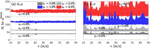
As a result of this study, Figures 8 and 9 show for all considered structures sample size N_l needed to estimate (a) mean and (b) standard deviation of the peak deflection and peak acceleration, respectively, for different relative slope criteria $s_r^{(\mathit{limit})}=\{0.005,0.01,0,025,0.05\}$ (plotted in red, blue, light and dark grey, respectively) as a function of the train speed. The black lines represent the average of the required sample size. It is observed that the required sample size, N_l, depends strongly on slope criterion $s_r^{(\mathit{limit})},$ and its average (for each $s_r^{(\mathit{limit})}$ separately considered) is similar for all considered statistical response quantities and virtually independent of speed v. Furthermore, the dispersion of N_l with respect to speed v is small for the mean peak response, but more pronounced for the standard deviations, especially of the peak acceleration. The most important finding of this study is that a single sample size N_l of irregularity profiles can be used for a parametric response study, depending only on $s_r^{(\mathit{limit})}$ but independent of parameter combination and train speed v. These outcomes show that 150 random irregularity profiles (i.e. N_l = 150, indicated in Figures 8 and 9 by a horizontal dashed line) are needed to capture the bridge response statistics. For this number of profiles, the peak acceleration standard deviation exceeds slope limit $s_r^{(\mathit{limit})}=1.0\%$ only for a few parameter combinations. A further increase of the sample size beyond this slope limit increases only marginally the accuracy, as it has been already shown in the previous analysis on the first case study object.

Figure 8. Sample size of irregularity profiles to satisfy different relative slope convergence criteria for the deflection response statistics.

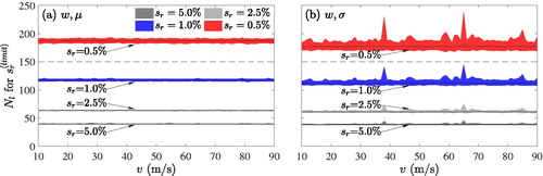
Figure 9. Sample size of irregularity profiles to satisfy different relative slope convergence criteria for the acceleration response statistics.

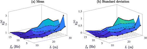
To support the choice of sample size N_l = 150, as additional evaluation criteria the 95% confidence boundaries (CBs) of the converged response statistics are determined. In Figure 10, the CBs of mean (left subfigure) and standard deviation (right subfigure) peak deflection (red lines with square markers) and peak acceleration (blue lines with circular markers) are plotted against the underlying resample size up to 150 profiles. Solid lines refer to the average CB values of all computed bridge samples, and the upper envelopes of the CBs are displayed by dashed lines. As observed, the CBs of the mean peak deflection are very small, with a maximum average of 1.1%. For 25 profiles, the CBs are always smaller than 5%, which is considered as a reasonable accuracy. Similarly, the average CB of the mean peak acceleration is less than 5% for 13 profiles only, and in all analysed samples less than 10% for 73 profiles, a number far below the proposed number of 150 irregularity profiles.

Figure 10. 95% confidence boundaries of the converged response statistic for (a) mean and (b) standard deviation of the peak deflection and peak acceleration response.

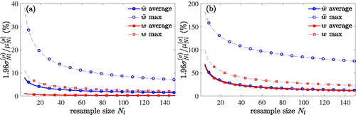
As expected, the CBs of the response standard deviations are larger. The CBs based on the average standard deviations of peak deflection and peak acceleration are both about 11% for N_l = 150. The maximum standard deviations show much higher CBs, that is 23% for the peak deflection and 75% for the peak acceleration for largest number of considered profiles. Since the slope of the CBs curves is quite small at the largest number of 150 profiles, a further increase of the sample size yields only a minor gain in accuracy. It is, thus, confirmed that 150 random profiles are sufficient to derive reasonably accurate the statistical bridge response.

3.4 Stochastic model for the bridge response

In a stochastic approach, the bridge response needs to be expressed in terms of appropriate probability distributions, which are subsequently identified. Basis for estimating the probability distribution are the $1.968\times {10}^4$ initial samples with size $N_0=1000$ of the peak bridge displacement and acceleration, determined for each bridge parameter combination and considered discrete train speed.

The histograms of the peak deflection and the corresponding fitted normal distributions of the case study object crossed by the train model with two different speeds depicted in Figure 11(a) provide visual evidence that this response quantity can be treated as normally distributed. Application of a ${\chi }^2$ goodness-of-fit test with a common 5% significance level shows that the assumption of a normal distribution is not rejected at 86.3% of all analysed parameter combinations and speeds, and yields an average p-value of 42.2%. At the lower speed depicted in Figure 11(a), $V_1=24$ m/s, the p-value ($=0.767$) of the fitted distribution is above the 5% significance level, indicating that this distribution is appropriate. For the higher speed, $V_2=28$ m/s, the p-value ($=0.032$) is below the significance level, but the normal distribution still provides an acceptable description of the response variation.

Figure 11. Histograms and fitted probability distributions for (a) the deflection and (b) the acceleration response for selected train speeds. Base case bridge model.

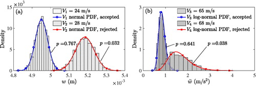
An extreme value distribution would be an appropriate model to capture the random peak acceleration response, with a 65.3% acceptance rate for all analysed bridges and train speeds, and an average p-value of 23.4%. As a drawback, for an extreme value distribution additionally to mean μ and standard deviation σ also a skewness parameter needs to be defined. Thus, in the present study, the statistical peak acceleration is fitted to a log-normal distribution, which is based on μ and σ only. This assumption is not rejected for 52.3% of all considered samples and train speeds with an average p-value of 20.8% and, thus, slightly less appropriate than the extreme value distribution. As an example, Figure 11(b) shows for the case study object histograms and corresponding fitted log-normal distribution of the peak acceleration induced by trains with speeds of $V_3=65$ m/s and $V_4=68$ m/s, respectively. These speeds have been selected to show the response distribution for an accepted and for a rejected ${\chi }^2$-test. In the first case, the p-value ($=0.641$) exceeds the 5% significance level of the fitted distribution, whereas in the second case the p-value ($=0.038$) falls below this level.

4. Assessment of the dynamic bridge response amplification due to rail irregularities

4.1 Parametric study

After identification of the required sample size of irregularity profiles, subsequently the effect of rail imperfections on the amplification of the dynamic bridge response is investigated. Amplification coefficients are defined as the ratio of dynamic peak response of the bridge with irregular tracks to the corresponding reference response quantity of the perfect bridge, (18) $${\chi }_w=\frac{w}{w_{\mathit{ref}}} ,{\chi }_{\ddot{w}}=\frac{\ddot{w}}{{\ddot{w}}_{\mathit{ref}}}$$(18)

In this equation, χ_w denotes the peak deflection amplification coefficient and ${\chi }_{\ddot{w}}$ the peak acceleration amplification coefficient. Since for the desired stochastic response assessment mean and standard deviation of the amplification factors are of primary interest, these statistics are subsequently computed from samples with 150 profiles each.

The boundaries of the considered parameter domain coincide with the ones of the previous study, where the required number of irregularity profiles has been identified. However, the resolution of span-frequency parameter combinations is higher, as indicated in Figure 2(a) by additional triangle markers. At each discrete span, five equally spaced fundamental bridge frequencies are considered, where the smallest natural frequency ($f_g^{(1)}$) corresponds to the lower frequency bound specified in EN1991-2 (2003) and the largest frequency ($f_g^{(5)}$) to the upper frequency bound.

In all subsequent figures, the style of the graphs representing the results is the same as for the corresponding frequency-span relations ($f_g^{(1)},\dots ,f_g^{(5)}-L$) shown in Figure 2(a). The considered bridge mass is a function of the bridge span only as shown in Figure 2(b). Three damping values as specified in Table 1, and spectral amplitudes for high, moderate and poor quality rails, $Q_r(a=\{0,0.5,1\}),$ complete the considered parameter space. All parameter combinations yield $9*5*3^3=1215$ bridge–train systems. For each of these systems, 150 samples with random irregularity profiles are generated. All 182250 samples are subjected to the Railjet train model with 81 different speeds equally spaced in the range $10\le v\le 90$ m/s. In total, for this parametric study $9*5*3^3*150*81=1.476\times {10}^7$ response history analyses are conducted.

4.2 Peak deflection amplification

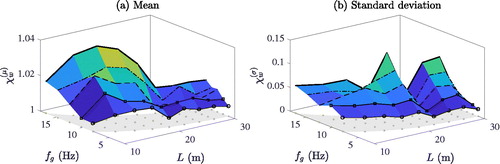
Figure 12 shows the maximum of (a) the mean and (b) the standard deviation peak deflection amplification, ${\chi }_w^{(\mu )}$ and ${\chi }_w^{(\sigma )},$ respectively, for the objects with minimum damping ${\zeta }_{D1}$ and poor rail quality $Q_r(1.0)$ as a function of fundamental frequency f_g and span L. The depicted amplification statistics represent the maximum values of all objects covering the entire mass and speed range. Thus, mean and standard deviations depicted in this figure do not necessarily belong to the same parameter combination. The chosen presentation of the response amplification χ with respect to f_g over L allows a comparison with design code recommendations such as Equation (1)(1) $$\phi ″=\frac{\alpha }{100}[56e^{-{(L/10)}^2}+50(\frac{L{f}_g}{80}-1\left)e^{-{(L/20)}^2}\right] , \alpha =\min \{v/22,1\}$$(1) . It is readily observed that the largest mean peak deflection of bridges with irregular profiles is only 4% larger than the corresponding response of the structure with perfect rails, that is ${\chi }_w^{(\mu )}=1.04$ at L = 15.0 m and $f_g^{(5)}=11.14$ Hz. Globally, ${\chi }_w^{(\mu )}$ tends to increase slightly with increasing fundamental frequency. Bridges of about L = 15.0 m span exhibit the largest mean deflection, whereas structures of span $L\ge 15.0$ m exhibit mean amplifications of around 1% only. In contrast, the largest standard deviations, ${\chi }_w^{(\sigma )},$ are in general related to longer bridge spans $L\ge 15.0$ m, with its maximum value ${\chi }_w^{(\sigma )}=0.13$ at L = 20.0 m and $f_g^{(5)}=10.08$ Hz. However, very close to this parameter domain, at L = 22.5 m, ${\chi }_w^{(\sigma )}$ has a local minimum independent of f_g. The reason behind this result is that for bridges of this span there are no significant resonance peaks in the considered speed range. As already observed previously, in a state of resonance, the response amplification and dispersion, and thus the standard deviation, are more pronounced. The resonance speed is a function of vehicle length d_v, and hence, the position of this local minimum in the parameter space depends on the crossing train type.

Figure 12. Maximum statistical amplification of the peak deflection due to random rail irregularities for lower bound damping ${\zeta }_{D1}$ and poor rail quality $Q_r(1.0).$

In a stochastic approach, the assessment of a certain limit state of a structure is conducted in the framework of the theory of probability. Since the deflection of a railway bridge is limited to avoid train derailment and to ensure passenger comfort, the maximum lateral bridge displacement is associated with a SLS. According to EN1990 (2013), the corresponding probability of exceedance is $p_f={10}^{-3}.$ From the point of view of such stochastic limit state assessment, subsequently response amplification factor χ_w is described as a normally distributed random variable (characterised by ${\chi }_w^{(\mu )}$ and ${\chi }_w^{(\sigma )}$), as found in the previous section. This allows to assign a probability of exceedance p_f to χ_w. Assuming a normal distribution $\mathcal{N}(\mu ,{\sigma }^2)$ for random variable χ_w, with cumulative distribution function $\Phi ,$ mean $\mu ={\chi }_w^{(\mu )}$ and standard deviation $\sigma ={\chi }_w^{(\sigma )},$ the amplification ${\chi }_w^{(\text{SLS})}$ at an exceedance probability of $p_f={10}^{-3}$ (related to the SLS) is computed as (Benjamin & Cornell, 2014) (19) $${\chi }_w^{\left(\text{SLS}\right)}={\Phi }^{-1}(1-p_f)={\chi }_w^{\left(\mu \right)}+3.0902{\chi }_w^{\left(\sigma \right)}$$(19)

Figure 13 shows the maximum of quantity ${\chi }_w^{(\text{SLS})}$ of all systems with different mass and all trains speeds, with respect to span L and fundamental bridge frequency f_g. Each subplot corresponds to a different combination of underlying damping coefficient and rail quality. The results of the first row are based on the lowest damping coefficient ${\zeta }_{D1},$ the ones of the second row on the largest damping coefficient ${\zeta }_{D3}.$ The rail quality assigned to the models is decreasing column-wise from high $Q_r(0),$ medium $Q_r(0.5)$ to poor $Q_r(1.0).$ The largest value of ${\chi }_w^{(\text{SLS})}$ of 1.30 appears in Figure 13(c) and corresponds to the following parameter combination: L = 20.0 m, $f_g^{(5)}=10.08$ Hz, ${\zeta }_{D3}$ (low damping) and $Q_r(1.0)$ (poor rail quality). As observed, in general the amplification factor increases with increasing frequency and also shows the same minimum as the standard deviation at L = 22.5 m. The peaks and valleys of the depicted amplification factor are related to the presence or absence of significant resonance peaks within the spectral response. 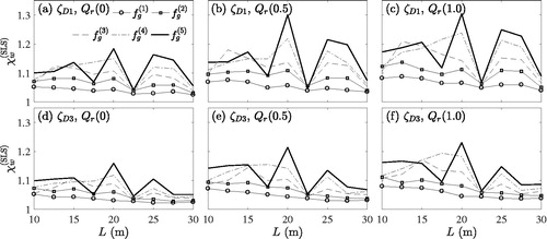The increase of deflection amplification for rail quality $Q_r(0.5)$ to rail quality $Q_r(1.0)$ is in average 1.6%, and thus, smaller than the average increase of 2.4% for $Q_r(0)$ to $Q_r(0.5).$ It is also seen that the difference of ${\chi }_w^{(\text{SLS})}$ related to minimum and maximum structural damping becomes larger with increasing rail quality, that is −1.7% and −2.7%, respectively, for the two extreme cases (a-d) and (c-f).

Figure 13. Maximum peak deflection amplification with an exceedance probability of $p_f={10}^{-3}$ for speeds up to $v\le 90$ m/s. Lower and upper bound of bridge damping. Three different rail qualities.

4.3 Peak acceleration amplification

Figure 14 shows the maximum of the (a) mean and (b) the standard deviation peak acceleration amplification, ${\chi }_{\ddot{w}}^{(\mu )}$ and ${\chi }_{\ddot{w}}^{(\sigma )},$ respectively, of all bridges with poor rail quality, $Q_r(1.0),$ and lower bound bridge damping ${\zeta }_{D1}$ subjected to the train model with all considered train speeds as a function of the fundamental frequency f_g and span L. It is readily seen that for a large parameter range, the mean and standard deviation peak acceleration amplification is significant, in contrast to the peak deflection amplification. The largest mean peak acceleration amplification of ${\chi }_{\ddot{w}}^{(\mu )}=3.20$ and the largest standard deviation acceleration amplification of ${\chi }_{\ddot{w}}^{(\sigma )}=1.29$ occur at the same parameter combination of L = 30.0 m and $f_g^{(2)}=4.22$ Hz. That is, irregular rails of poor quality lead to an increase of the mean peak acceleration by 320% compared to the perfect bridge. For comparison, the gain of the maximum mean peak deflection has been 4% only. The global evolution of the statistical values of the peak acceleration and peak deflection with respect to f_g and L is different, compare Figure 12 with Figure 14. Here, a non-continuous increase of both ${\chi }_{\ddot{w}}^{(\mu )}$ and ${\chi }_{\ddot{w}}^{(\sigma )}$ with increasing span is observed.

Figure 14. Maximum statistical amplification of the acceleration response due to random rail irregularities for lower bound damping ${\zeta }_{D1}$ and poor rail quality $Q_r(1.0).$

Subsequently, for a stochastic response assessment peak acceleration amplification ${\chi }_{\ddot{w}}$ is treated as a log-normally distributed random quantity, as previously demonstrated. The cumulative distribution function $F_{\chi }({\chi }_{\ddot{w}})$ of the peak acceleration amplification is, thus, defined as (Benjamin & Cornell, 2014) (20) $$F_{\chi }\left({\chi }_{\ddot{w}}\right)=\Phi \left(\frac{\hspace{0.17em}\text{log}\hspace{0.17em}{\chi }_{\ddot{w}}-m_{\mathit{LN}}}{s_{\mathit{LN}}}\right) , m_{\mathit{LN}}=\hspace{0.17em}\text{log}\hspace{0.17em}\left(\frac{{\chi }_{\ddot{w}}^{\left(\mu \right)}}{\sqrt{1+{\chi }_{\ddot{w}}^{\left(\sigma \right)2}/{\chi }_{\ddot{w}}^{\left(\mu \right)2}}}\right) , s_{\mathit{LN}}^2=\hspace{0.17em}\text{log}\hspace{0.17em}(1+\frac{{\chi }_{\ddot{w}}^{\left(\sigma \right)2}}{{\chi }_{\ddot{w}}^{\left(\mu \right)2}})$$(20)

The peak acceleration amplification factors associated with a specific probability of exceedance are governed by the relation (Benjamin & Cornell, 2014) (21) $${\chi }_{\ddot{w}}^{\left(\text{SLS}\right)}=F_{\chi }^{-1}(1-p_f)$$(21)

This relation considers that the exceedance of the maximum admissible acceleration of a ballasted railway bridge is also a SLS (Rocha et al., 2014; Salcher et al., 2016) related to the exceedance probability $p_f={10}^{-3}$ (see EN1990, 2013).

Figure 15 shows ${\chi }_{\ddot{w}}^{(\text{SLS})}$ for the worst case scenario of lower bound damping and poor rail quality, and three different maximum speed limits, that is (a) $v\le 56.0$ m/s ($\approx$ 200 km/h), (b) $v\le 70.0$ m/s ($\approx$ 250 km/h) and (c) $v\le 84.0$ m/s ($\approx$ 300 km/h), plotted against span L. Each of the five lines corresponds to a span-dependent fundamental bridge frequency $f_g^{(i)},i=1,\dots ,5$ depicted in Figure 2(a). Comparing subplots (a), (b) and (c) reveals that for longer bridges quantity ${\chi }_{\ddot{w}}^{(\text{SLS})}$ increases significantly when the upper speed limit becomes higher. In contrast, short objects in the range between L = 10.0 and L = 12.5 m, amplification factor ${\chi }_{\ddot{w}}^{(\text{SLS})}$ is in general much smaller and almost not affected by the upper speed limit. Another observation is that ${\chi }_{\ddot{w}}^{(\text{SLS})}$ tends to become larger with increasing span L and also with increasing frequency f_g. The largest value of ${\chi }_{\ddot{w}}^{(\text{SLS})}=7.10$ is related to span L = 25.0 m, frequency $f_g^{(5)}=8.53$ Hz and the largest upper speed limit $v\le 84.0$ m/s, as seen in Figure 15(c). For the lowest upper speed boundary, $v\le 56.0$ m/s, ${\chi }_{\ddot{w}}^{(\text{SLS})}$ is 4.48, indicating a peak acceleration amplification of more than 400%. The corresponding span and fundamental frequency are L = 30.0 m and $f_g^{(5)}=7.44$ Hz. It should be noted that, although these amplifications are quite large compared to the deflection amplifications, such significant amplification coefficients do not necessarily imply large absolute peak accelerations $\ddot{w}$ if the ones of the corresponding perfect bridge are very small. For instance, the latter discussed amplification factor of 4.48 corresponds in the speed range $10.0\le v\le 56.0$ m/s to a maximum peak acceleration of $\ddot{w}=2.24$ m/s², which is still far beyond the acceleration limit of 3.5 m/s² specified in EN1991-2 (2003) for ballasted bridges. On the other hand, amplification ${\chi }_{\ddot{w}}^{(\text{SLS})}=2.16$ at frequency $f_g^{(5)}$ and span L = 12.5 m results in a peak acceleration $\ddot{w}=4.56$ m/s², exceeding the specified design limit in the speed range $10.0\le v\le 84.0$ m/s.

Figure 15. Maximum peak acceleration amplification with an exceedance probability of $p_f={10}^{-3}.$ Speed range (a) $10.0\le v\le 56.0$ m/s, (b) $10.0\le v\le 70.0$ m/s, (c) $10.0\le v\le 84.0$ m/s. Lower bound of bridge damping ${\zeta }_{D1}.$ Poor rail quality $Q_r(1.0).$

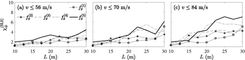
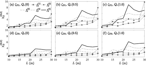
The influence of bridge damping and rail quality on ${\chi }_{\ddot{w}}^{(\text{SLS})}$ is visualised in Figure 16. The results are organised in the same manner as in Figure 15, capturing the maximum considered speed range $10.0\le v\le 90.0$ m/s. Each subplot corresponds to a different combination of underlying damping coefficient and rail quality, compare with Figure 15. As expected, the general shape of ${\chi }_{\ddot{w}}^{(\text{SLS})}$ is not much affected by damping and rail quality, but the amplitudes of ${\chi }_{\ddot{w}}^{(\text{SLS})}$ strongly depend on these parameters. For the most favourable combination of upper bound damping and high rail quality, the maximum amplification ${\chi }_{\ddot{w}}^{(\text{SLS})}$ is 3.73 (Figure 16(b)), whereas minimum damping and poor rail quality lead to an overall maximum peak acceleration amplification of ${\chi }_{\ddot{w}}^{(\text{SLS})}=9.82.$ It is observed that peak acceleration amplification ${\chi }_{\ddot{w}}^{(\text{SLS})}$ of short span bridges $10.0\le L\le 12.5$ m is not much affected by damping and rail quality. Comparing the outcomes of this figure with the ones of Figure 13 reveals that in the span range $22.5\le L\le 30.0$ m the peak acceleration amplifications are largest, whereas the peak deflection amplifications are smallest.

Figure 16. Amplification of the acceleration response with an exceedance probability of $p_f={10}^{-3}$ for speeds $v\le 90$ m/s for minimum and maximum bridge damping and three different rail qualities.

4.4 Comparison of the amplified response

In this section, the computed amplifications of the dynamic response at the exceedance limit, ${\chi }_w^{(\text{SLS})}$ and ${\chi }_{\ddot{w}}^{(\text{SLS})},$ are set in contrast to the recommendations of EN1991-2 (2003). To this end, in Figure 17 the amplification factors are depicted as a 3D plot with respect to span L and frequency f_g both for the most favourable (upper bound damping ${\zeta }_{D3}$/good quality rails $Q_r(0),$ plotted in red) and the most unfavourable parameter combination (lower bound damping ${\zeta }_{D1}$/poor rail quality $Q_r(1.0),$ plotted in blue). Alternatively, Figure 18 shows the same amplification factors for discrete frequencies $f_g^{(1)},\dots ,f_g^{(5)}$ as a function of span L. The amplification factors are related to the full speed range $v\le 90$ m/s. Comparing the left subplots with the ones of the right-hand side demonstrates that the amplifications at the exceedance limits for the peak bridge acceleration are much larger than for the peak deflection. Additionally, amplification factor ${\chi }^{(\text{EC})}=1+\phi ″$ according to Equation (1)(1) $$\phi ″=\frac{\alpha }{100}[56e^{-{(L/10)}^2}+50(\frac{L{f}_g}{80}-1\left)e^{-{(L/20)}^2}\right] , \alpha =\min \{v/22,1\}$$(1) , which is recommended in the Eurocode EN1991-2 (2003) for standard maintenance, is illustrated by black lines. Note that this design factor is the same for all response quantities.

Figure 17. Amplification factor for (a) the deflection and (b) the acceleration related to an exceedance probability of $p_f={10}^{-3}$ compared to a design recommendation ${\chi }^{(\text{EC})}$ (EN1991–2, 2003). Most favourable and most unfavourable parameter combination.

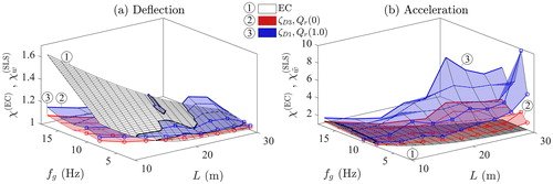
Figure 18. Amplification factor for (a) the deflection and (b) the acceleration related to an exceedance probability of $p_f={10}^{-3}$ for natural frequency relations $f_g^{(1)},\dots ,f_g^{(5)}$ as a function of span L compared to a design recommendation ${\chi }^{(\text{EC})}$ (EN1991–2, 2003). Most favourable and most unfavourable parameter combination. Line styles for the individual combinations according to Figure 2.

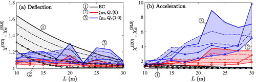
As observed, the overall evolution of ${\chi }_w^{(\text{SLS})}$ and of ${\chi }^{(\text{EC})}$ with respect to parameters L and f_g is similar, that is both increase in general with increasing frequency and decreasing span. For long bridges with the most unfavourable parameter combination, code factor ${\chi }^{(\text{EC})}$ underestimates the computed amplification factor. In contrast, for short span bridges, ${\chi }^{(\text{EC})}$ yields a conservative prediction of the peak deflection amplification.

The right plots of Figure 17 and Figure 18 reveal that the derived peak acceleration response amplification factor is in almost the entire parameter domain many times larger than the design code recommendation. Only for the shortest bridges, where ${\chi }^{(\mathit{EC})}$ is largest with values from 1.21 to 1.62, the code recommendation delivers predictions close to the ones derived in this study. For longer spans, the amplifications due to random rail irregularities increase in contrast to the code factor and hence highly exceed the later.

5. Conclusions

The impact of random rail irregularities, modelled as a stationary Gaussian process in space, on the dynamic response of simple railway bridges was studied. Randomly generated rail profiles were assigned to a planar plane bridge–vehicle interaction model. The results of this study are based on a single train type, whose specific excitation frequencies depend on the axle spacing. The regular car length of the considered Railjet train model is, however, representative for other common high-speed trains. In parametric studies considering bridges with spans between 10 and 30 m, crude Monte Carlo simulations on random samples of this model yielded mean and standard deviations of the bridge peak deflection and peak acceleration. Application of a modified bootstrap method revealed that 150 random rail irregularity profiles are required to describe the acceleration response statistics sufficiently accurate. The variability of the peak deflection is captured by a smaller number of irregularity profiles. The results depend also on the considered irregularity PSD function and its range of wavelength. However, the major findings and conclusions of this contribution remain unaffected from these choices and assumptions.

It was shown that the scatter of the dynamic peak bridge deflection considering irregular rail profiles can be modelled as normally distributed variable, whereas for the acceleration response a log-normal distribution approximates more appropriately the variability of this quantity. Based on these simple stochastic approximations, response amplification factors were derived, which describe the amplification due to rail irregularities compared to response of the corresponding bridge with perfect rails. These amplification factors allow to relate the effects of irregular rail surfaces with the exceedance probability of the SLS.

One major conclusion of this study is that in the considered parameter domain the amplification of the response strongly depends on the considered response quantity, and thus, for each quantity a different design amplification factor should be used. The peak deflection increases with decreasing span, whereas the acceleration response becomes larger with increasing bridge length. The amplification of the peak deflection depends on the resonance peaks of the reference bridge with perfect rail. The extension of the upper speed limit led to a major increase of the bridge acceleration amplification. The latter effects are both related to critical resonance speeds and thus also to the geometry of the crossing train.

It was found that the established design factor recommended in the Eurocode (based on isolated rail pumps) captures globally the amplification of the lateral deflection due to irregular rails. However, this design factor yields in the most cases extremely unconservative predictions of the dynamic peak acceleration amplification. In this context, novel design amplification factors for the acceleration response need to be established based on extensive parameter studies comprising various bridge and train models of various degrees of sophistication.

Acknowledgement

The computational results presented have been achieved in part using the HPC infrastructure LEO of the University of Innsbruck.

Disclosure statement

No potential conflict of interest was reported by the authors.

References

- Adam, C., & Salcher, P. (2014). Dynamic effect of high-speed trains on simple bridge structures. Structural Engineering and Mechanics, 51(4), 581–599. doi: 10.12989/sem.2014.51.4.581
- Antolín, P., Zhang, N., Goicolea, J. M., Xia, H., Astiz, M. A., & Oliva, J. (2013). Consideration of nonlinear wheel–rail contact forces for dynamic vehicle–bridge interaction in high-speed railways. Journal of Sound and Vibration, 332(5), 1231–1251. doi: 10.1016/j.jsv.2012.10.022
- Arvidsson, T., Andersson, A., & Karoumi, R. (2019). Train running safety on non-ballasted bridges. International Journal of Rail Transportation, 7(1), 1–22. doi: 10.1080/23248378.2018.1503975
- Au, F., Wang, J., & Cheung, Y. (2002). Impact study of cable-stayed railway bridges with random rail irregularities. Engineering Structures, 24(5), 529–541. doi: 10.1016/S0141-0296(01)00119-5
- Benjamin, J. R., & Cornell, C. A. (2014). Probability, statistics, and decision for civil engineers. Mineola, NY: Dover Publications.
- Biondi, B., Muscolino, G., & Sofi, A. (2005). A substructure approach for the dynamic analysis of train–track–bridge system. Computers & Structures, 83(28–30), 2271–2281. doi: 10.1016/j.compstruc.2005.03.036
- Cantero, D., Arvidsson, T., OBrien, E., & Karoumi, R. (2016). Train–track–bridge modelling and review of parameters. Structure and Infrastructure Engineering, 12(9), 1051–1065. doi: 10.1080/15732479.2015.1076854
- Cantero, D., Hester, D., & Brownjohn, J. (2017). Evolution of bridge frequencies and modes of vibration during truck passage. Engineering Structures, 152, 452–464. doi: 10.1016/j.engstruct.2017.09.039
- Cantero, D., & Karoumi, R. (2016). Numerical evaluation of the mid-span assumption in the calculation of total load effects in railway bridges. Engineering Structures, 107, 1–8. doi: 10.1016/j.engstruct.2015.11.005
- Claus, H., & Schiehlen, W. (1998). Modeling and simulation of railway bogie structural vibrations. Vehicle System Dynamics, 29(Supp. 1), 538–552. doi: 10.1080/00423119808969585
- Colaço, A., Costa, P. A., & Connolly, D. P. (2016). The influence of train properties on railway ground vibrations. Structure and Infrastructure Engineering, 12(5), 517–534. doi: 10.1080/15732479.2015.1025291
- Davison, A. C., & Hinkley, D. V. (1997). Bootstrap methods and their application (Vol. 1). Cambridge: Cambridge University Press.
- Doménech, A., Museros, P., & Martínez-Rodrigo, M. D. (2014). Influence of the vehicle model on the prediction of the maximum bending response of simply-supported bridges under high-speed railway traffic. Engineering Structures, 72, 123–139. doi: 10.1016/j.engstruct.2014.04.037
- Efron, B. (1979). Bootstrap methods: Another look at the jackknife. The Annals of Statistics, 7(1), 1–26. doi: 10.1214/aos/1176344552
- EN13848-5. (2010). Eurocode: EN13848–5: Railway applications – track – track geometry quality – Part 5 – Geometric quality levels – Plain line: European Committee for Standardization.
- EN1990. (2013). Eurocode 0: EN1990: Basis of structural design – Amendment 1: Application for bridges: European Committee for Standardization.
- EN1991-2. (2003). Eurocode 1: EN 1991–2: Actions on structures: European Committee for Standardization: ÖBB Infrastruktur.
- Frýba, L. (1996). Dynamics of Railway Bridges. London: Thomas Telford Publishing.
- Gulvanessian, H., Formichi, P., Calgaro, J.-A., & Harding, G. (2009). Designers’ guide to Eurocode 1. London: Thomas Telford Services Ltd.
- Johansson, C., Nualláin, N. Á. N., Pacoste, C., & Andersson, A. (2014). A methodology for the preliminary assessment of existing railway bridges for high-speed traffic. Engineering Structures, 58, 25–35. doi: 10.1016/j.engstruct.2013.10.011
- Kuisle, A. (2018). Numerische Studie zum Einfluss zufälliger Gleisunebenheiten auf die Dynamik einfacher Eisenbahnbrücken [in German,” Numerical study on the impact of random rail irregularities on the dynamic response of simple railway bridges”] (Master’s thesis). University of Innsbruck.
- Lei, X., & Noda, N. A. (2002). Analyses of dynamic response of vehicle and track coupling system with random irregularity of track vertical profile. Journal of Sound and Vibration, 258(1), 147–165. doi: 10.1006/jsvi.2002.5107
- Majka, M., & Hartnett, M. (2009). Dynamic response of bridges to moving trains: A study on effects of random track irregularities and bridge skewness. Computers & Structures, 87(19–20), 1233–1252. doi: 10.1016/j.compstruc.2008.12.004
- Malveiro, J., Sousa, C., Ribeiro, D., & Calcada, R. (2018). Impact of track irregularities and damping on the fatigue damage of a railway bridge deck slab. Structure and Infrastructure Engineering, 14(9), 1257–1268. doi: 10.1080/15732479.2017.1418010
- Moyo, P., & Tait, R. (2010). Structural performance assessment and fatigue analysis of a railway bridge. Structure and Infrastructure Engineering, 6(5), 647–660. doi: 10.1080/15732470903068912
- Nielsen, J., & Igeland, A. (1995). Vertical dynamic interaction between train and track influence of wheel and track imperfections. Journal of Sound and Vibration, 187(5), 825–839. doi: 10.1006/jsvi.1995.0566
- ÖBB-RLI-Dynamik. (2011). ÖBB Infrastruktur: Richtlinie für die dynamische Berechnung von Eisenbahnbrücken [in German, Guideline for the dynamic analysis of railway bridges].
- Rocha, J. M., Henriques, A. A., & Calçada, R. (2014). Probabilistic safety assessment of a short span high-speed railway bridge. Engineering Structures, 71, 99–111. doi: 10.1016/j.engstruct.2014.04.018
- Rocha, J. M., Henriques, A. A., & Calcada, R. (2016). Probabilistic assessment of the train running safety on a short-span high-speed railway bridge. Structure and Infrastructure Engineering, 12(1), 78–92. doi: 10.1080/15732479.2014.995106
- Salcher, P. (2015). Reliability assessment of railway bridges designed for high-speed traffic: Modeling strategies and stochastic simulation (Doctoral thesis). University of Innsbruck.
- Salcher, P., & Adam, C. (2015). Modeling of dynamic train-bridge interaction in high-speed railways. Acta Mechanica, 226(8), 2473–2495. doi: 10.1007/s00707-015-1314-6
- Salcher, P., & Adam, C. (2018). Ein Bemessungsbehelf zur schnellen dynamischen Bewertung von einfachen Eisenbahnbrücken [in German,” Design charts for a quick dynamic assessment of simple railway bridges”]). Bauingenieur, 93(6), 233–241.
- Salcher, P., Pradlwarter, H., & Adam, C. (2016). Reliability assessment of railway bridges subjected to high-speed trains considering the effects of seasonal temperature changes. Engineering Structures, 126, 712–724. doi: 10.1016/j.engstruct.2016.08.017
- Xia, H., Zhang, N., & Guo, W. W. (2006). Analysis of resonance mechanism and conditions of train–bridge system. Journal of Sound and Vibration, 297(3–5), 810–822. doi: 10.1016/j.jsv.2006.04.022
- Yang, Y. B., Yau, J. D., & Wu, Y. S. (2004). Vehicle–bridge interaction dynamics. Singapore: World Scientific Publishing Company.
- Yu, Z.-W., Mao, J.-F., Guo, F.-Q., & Guo, W. (2016). Non-stationary random vibration analysis of a 3D train-bridge system using the probability density evolution method. Journal of Sound and Vibration, 366, 173–189. doi: 10.1016/j.jsv.2015.12.002
- Zhang, N., Xia, H., Guo, W. W., & De Roeck, G. (2010). A vehicle–bridge linear interaction model and its validation. International Journal of Structural Stability and Dynamics, 10(02), 335–361. doi: 10.1142/S0219455410003464
- Ziegler, F. (1998). Mechanics of solids and fluids (3rd ed.). New York: Springer.