Investigation of the effect of the inspection intervals on the track geometry condition

Abstract

In order to evaluate the railway track geometry condition and plan maintenance activities, track inspection cars run over the track at specific times to monitor it and record geometry measurements. Applying an adequate inspection interval is vital to ensure the availability, safety and quality of the railway track, at the lowest possible cost. The aim of this study has been to investigate the effect of different inspection intervals on the track geometry condition. To achieve this, an integrated statistical model was developed to predict the track geometry condition given different inspection intervals. In order to model the evolution of the track geometry condition, a piecewise exponential model was used which considers break points at the maintenance times. Ordinal logistic regression was applied to model the probability of the occurrence of severe isolated defects. The Monte Carlo technique was used to simulate the track geometry behaviour given different inspection intervals. The results of the proposed model support the decision-making process regarding the selection of the most adequate inspection interval. The applicability of the model was tested in a case study on the Main Western Line in Sweden.

Keywords:

• Inspection
• track geometry
• maintenance
• multivariable linear regression
• isolated defects
• ordinal logistic regression

1. Introduction

The railway track geometry is subjected to degradation mainly due to the forces induced by traffic, which cause deviations from the designed vertical and horizontal alignments. When a geometry defect occurs, the consequences can be significant, including economic loss, damage to the environment and, in severe cases, the possible loss of human lives. In order to protect against unacceptable consequences, track geometry maintenance actions are planned to retain the geometry condition in or restore it to an acceptable state with respect to ride comfort and the safety limits. In order to have an effective and efficient maintenance plan, the track geometry condition must be inspected on a regular basis. The main aims of geometry inspection are to determine the deviation of geometry parameters from acceptable limits, and to enable prediction of the time remaining until the intervention and safety limits are reached (UIC, 2008). The frequency of inspection is highly important as it affects the detectability of geometry defects and the associated maintenance requirements. As a result, a proper inspection interval is a key factor for determining the performance of line sections, controlling and reducing the risk of derailment and the maintenance cost, and keeping the punctuality of train operations at the highest level. Various factors are involved in the selection of an applicable and effective inspection interval, including the traffic profile, the regulatory requirements, the level of risk in train operations, and the maximum allowable speed of trains (American Railway Engineering and Maintenance-of-Way Association (AREMA), 2006).

In recent years, a number of researchers have tried to determine an optimal inspection interval with respect to different objective functions. Arasteh Khouy, Larsson-Kråik, Nissen, Juntti, and Schunnesson (2014) optimized the track geometry inspection intervals with the objective of minimizing the total maintenance cost. In the proposed model, preventive and corrective tamping is executed based on the Q-value indicator and severe defects of twist, respectively. A similar approach can be found in Soleimanmeigouni, Ahmadi, Letot, Nissen, and Kumar (2016), who attempted to determine a cost-effective track geometry inspection interval. They considered the standard deviation of the longitudinal level as the dominant factor for evaluation of the track condition. They used the Wiener process to model the track geometry degradation. Lyngby, Hokstad, and Vatn (2008) conducted research to optimize the intervals of track geometry inspection with the same objective. They applied the Markov methodology to model the track geometry degradation. In their study, twist was considered as a track quality indicator. In the model proposed by Lyngby et al. (2008), the corrective and preventive activities are assumed to be perfect. Meier-Hirmer, Sourget, and Roussignol (2005) conducted a case study and determined a trade-off between the inspection interval and the maintenance threshold that leads to the minimum track maintenance cost. The track geometry degradation and tamping effectiveness were modelled using the gamma process and linear regression, respectively. In this study, the maintenance was carried out on track sections with a fixed delay after detection.

More recently, Osman, Kaewunruen, Jack, and Sussman (2016) conducted research on the possibility of considering a ‘plan B’ or contingency plan in track inspection schedules. This ‘plan B’ would reschedule the inspection plan in the event of an incident happening which would affect the current inspection schedule. A different approach can be seen in a study presented by Andrews, Prescott, and De Rozières (2014), who did not include an objective function in their work. They studied the effect of different inspection strategies on the quality of the track geometry. The standard deviation of the longitudinal level was used as a measurement of the track geometry quality. They reported that, despite their expectations, different inspection intervals did not have a significant effect on the total number of maintenance actions. However, they ascertained that the longer the inspection intervals were, the larger was the proportion of maintenance which had to be carried out on track with poorer quality. Moreover, Andrews et al. (2014) pointed out that a decrease in the frequency of inspections would increase the percentage of time during which the track would need emergency maintenance.

Obviously, an effective inspection regime can be developed according to an assessment of the effect of different inspection intervals on the track performance. The performance of the track can be measured by determining the percentage of time spent by the track sections in different geometry states. These states can be defined based on the maintenance limits. The aim of the present study has been to develop an integrated approach to investigate the effect of different inspection intervals on the performance of the track. A fundamental requirement for achieving this aim is long-term prediction of the track geometry condition by modelling and integrating: (1) the track geometry degradation; (2) the tamping recovery; (3) the occurrence of severe isolated defects. In this study, to characterize the track geometry degradation and restoration, a piecewise exponential model was applied which considers break points at the maintenance times. A multivariable linear regression model was used to link different covariates to the tamping recovery. In addition, ordinal logistic regression was applied to predict the probability of the occurrence of isolated defects. Due to the existence of variation in the model parameters, the Monte Carlo technique was used to estimate the percentage of time spent in different track geometry states. In order to verify the applicability of the model, a case study was performed with data collected from the Main Western Line in Sweden.

The rest of this paper is organized as follows. Section 2 contains background information on the track geometry parameters and maintenance limits. Section 3 describes the process of track geometry measurement. Section 4 deals with the analytical models and the proposed approach. The case study is presented in Section 5 and, finally, Section 6 provides the conclusions.

2. Track geometry parameters and maintenance limits

Track geometry parameters are widely used to represent the track condition and to plan maintenance activities. Track geometry parameters can be divided into five classes, i.e. the longitudinal level, alignment, gauge, can’t, and twist. The longitudinal level is the geometry of the track centreline projected onto the longitudinal vertical plane. The alignment is the geometry of the track centreline projected onto the longitudinal horizontal plane. The gauge is the distance between the gauge faces of two adjacent rails at a given location below the running surface. The cant (cross-level) is the difference in height between the adjacent running tables computed from the angle between the running surface and a horizontal reference plane. The twist is the algebraic difference between two cross-levels taken at a defined distance apart, usually expressed as a gradient between the two points of measurement (SS-EN 13848-1: 2004 + A1, 2008).

According to EN 13848-5 (2008), there are three limits for maintenance actions. The immediate action limit (IAL) or safety limit refers to the value which, if exceeded, due to the potential risk of derailment, requires that a speed reduction or line closure be imposed before a corrective maintenance (CM) action is conducted. The intervention limit (IL) or CM limit refers to the value which, if exceeded, requires a CM action before the immediate action limit is reached. The alert limit (AL) or preventive maintenance (PM) limit refers to the value which, if exceeded, requires that the track geometry be analysed for the planning of future maintenance actions. The European standard EN 13848-5 (2008) provides the IALs, ILs and ALs for isolated defects and gives ALs for standard deviations. Generally, the track quality indices (TQIs) based on the standard deviation of track geometry parameters are used to plan and perform PM actions. On the other hand, the execution of CM actions is based on the severity of isolated defects. Whenever the amplitude of an isolated defect exceeds the IL or IAL, CM should be conducted on the track. Figure 1 shows the different maintenance zones based on the above-mentioned limits.

Figure 1. Different maintenance zones based on limits.

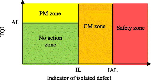
The IALs are normative and take into account the track-vehicle interaction and the risk of unexpected events, whereas the ILs and ALs are informative and are mainly linked with the maintenance policy. In fact, the ILs and ALs provided in EN 13848-5 (2008) reflect the common practice adopted by most European infrastructure managers. In alignment with the European standard EN 13848-5 (2008), Trafikverket (2015) has defined four main limits, namely the planning limit, the UH1 and the UH2 limit, and the critical limit, as can be seen in Figure 2. In Trafikverket (2015) the intervention limit is expressed as a range rather than as a discrete value. Track irregularities that exceed the UH1 limit must be assessed for conducting maintenance before the UH2 limit is exceeded. For track irregularities exceeding the UH2 limit, a maintenance action must be planned without unnecessary delay. Therefore, track irregularities must be corrected before the UH2 limit is reached. Table 1 presents the relation between the limits defined in EN 13848-5 (2008) and those defined in Trafikverket (2015).

Figure 2. Examples of UH1, UH2 and critical defects of the longitudinal level.

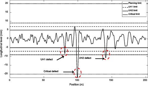
Table 1. Maintenance limits defined in the European standard EN 13848-5 and in Trafikverket (2015).

European standard EN 13848-5	Trafikverket (2015)
Alert limit	Planning limit
Intervention limit	UH1 limit (lower bound for corrective maintenance)
	UH2 limit (upper bound for corrective maintenance)
Immediate action limit	Critical limit

Based on the above-mentioned limits, geometry defects can be classified according to their severity into three groups, i.e. UH1, UH2 and critical defects. UH1, UH2 and critical defects occur when track irregularities exceed the UH1, UH2 and critical limits, respectively. Examples of these three categories of defects are shown in Figure 2.

3. Track geometry inspection

The main objectives of measuring the track geometry are to: (1) locate the occurrence of severe isolated defects and prioritize the CM actions required to rectify them, (2) to plan the PM actions, (3) to evaluate the effectiveness and quality of conducted maintenance activities, and (4) to establish the effectiveness and adequacy of financial expenditure (Zaayman, 2017). The track geometry measurement car is an automated track inspection vehicle whose purpose is to measure and record the track geometry in real time and to display the measurements obtained. The vehicle measures various geometry parameters, e.g. the longitudinal level, alignment, can’t, gauge, twist, curve radius, and gradient at a specific sampling interval.

The measured data are available in three forms, i.e. on-board network viewing of measurements, on-board real-time reports, and off-board post-processed reports. The on-board real-time reports can be used to address severe isolated defects and comprise strip charts and exceptions reports. The strip chart is a graphical representation of the overall track geometry condition in one picture and displays all the track geometry measurements and the corresponding maintenance limits. The strip chart shows when a particular measurement approaches or exceeds the maintenance limits. When the track geometry measurements exceed the maintenance limits, a geometry defect will appear in the exceptions report.

The purpose of the exceptions report is to provide a list of all the geometry defects found by the track geometry measurement vehicle during the inspection of the track. The basic information provided in the exceptions report is the defect name, the position of the defect, and the defect length, defect magnitude, maintenance limit, and maximum allowable speed. Using the strip charts and the exceptions reports aids the process of conducting CM activities to avoid the occurrence of severe isolated defects which may cause catastrophic consequences. In addition to on-board reports, the geometry measurements are post-processed into different standard reports. These reports can be used for further analysis of the track geometry condition to support track maintenance decision making to achieve a robust and cost-effective maintenance plan. Analysing the track geometry measurements and aggregating them into a track quality index (TQI) can aid the planning of track geometry maintenance activities. By performing a statistical analysis on the evolution of the TQIs, the trends in the track geometry degradation can be identified. In addition, the measured data can be used to identify potentially hazardous track geometry conditions.

4. Proposed methodology

Figure 3 provides a schematic description of the proposed analytical model. As can be seen, the track geometry is inspected at discrete time intervals ($\tau$) to determine its condition. At each inspection, the standard deviation of the geometry parameters and the extreme values of isolated defects are recorded. According to the results of the track geometry inspection, different intervention decisions can be made to retain the geometry condition in or to restore it to an acceptable state. With reference to the maintenance limits explained in Section 2, after each inspection, one of the following three actions may be taken.

Figure 3. Schematic description of preventive and corrective maintenance actions.

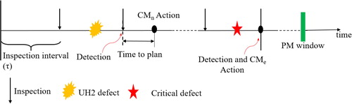
• Preventive maintenance: If the standard deviation of the geometry parameters exceeds the planning limit, then the track section is assessed for PM to be performed in the first available maintenance window. By scheduling the PM for the time periods planned for maintenance interventions, the maintenance will be performed in a way which will neither interrupt the normal traffic nor cause traffic delays.

• Normal corrective maintenance (CM_n): When a UH2 defect occurs, a CM action is conducted on the track section. Railway companies need short-term plans for adjusting the traffic by cancelling, postponing or rerouting trains to provide time to conduct CM actions. Such short-term plans provide a period of time during which the track can be operated until maintenance takes place.

• Emergency corrective maintenance (CM_e): When a critical defect occurs, an immediate CM action with a speed reduction or line closure is carried out on the track section.

Figure 3 depicts the three above-mentioned situations. The aim of the proposed analytical model is to predict the percentage of time which the track spends in the different track geometry states using various inspection intervals. With reference to the maintenance limits explained in Section 2, Table 2 presents the different geometry states. Owing to the complexity of the degradation process and the maintenance process, predicting the effect of employing different inspection intervals on the track geometry condition is a difficult task (Andrews et al., 2014; Quiroga & Schnieder, 2012). Therefore, the Monte Carlo simulation technique is used to handle the variation of the various parameters within the proposed integrated model and to estimate the percentage of time spent in the different track geometry states.

Table 2. Three defined track geometry states based on the maintenance limits.

State	Definition
1	There is no UH2 defect or critical defect in the track section.
2	There is at least one UH2 defect in the track section, but there is no critical defect in that section.
3	There is at least one critical defect in the track section.

4.1. Track geometry degradation and restoration

In order to model the evolution of the geometry condition of a track line over time, three main challenges must be addressed: (1) modelling the track geometry degradation within a maintenance cycle, (2) modelling the effect of tamping on the geometry degradation pattern, and (3) modelling the section-to-section variation in the degradation parameters. In order to model the track geometry evolution, the first level of the framework proposed by Soleimanmeigouni, Xiao, Ahmadi, Xie, Nissen, and Kumar (2018) was adapted.

Exponential model, with time or tonnage as the explanatory variable, is widely used in the literature to model track geometry degradation within a maintenance cycle (Soleimanmeigouni, Ahmadi, & Kumar, 2018). The main advantage of exponential model lies in its simplicity and ability to represent the underlying geometry degradation path. In this study, in order to model track geometry degradation of the section $s$ within a maintenance cycle an exponential model with a multiplicative lognormal error term is used: (1) $$D_s\left(t\right)=D_{s,0}{\mathrm{e}}^{{\beta }_{s}t}{ϵ}_s$$(1) where:

• $D_s\left(t\right)$ is the degradation value at time $t\in \mathcal{T},$

• $D_{s,0}>0$ is the initial degradation level,

• ${\mathrm{\beta }}_s>0$ is the degradation rate,

• ${ϵ}_s$ is the random error term following a lognormal distribution with the location parameter zero and the scale parameter ${\sigma }_s.$

When the degradation characteristic reaches the maintenance threshold, tamping action will be scheduled to restore the track geometry condition. The geometry degradation path always has a break point after a tamping action. Although tamping actions will improve the track geometry condition, they cannot rejuvenate the geometry condition to an as-good-as-new state. Therefore, in order to predict the track geometry evolution in multiple maintenance cycles, the effect of tamping on track geometry degradation must be assessed. The recovery value after tamping intervention is a function of different covariates, e.g. degradation value before tamping and number of accumulated tamping interventions. In this study, multivariable linear regression was used to explain the relationship between the covariates and the recovery value after tamping as follows: (2) $${\mathrm{R}}_{\mathrm{j},\mathrm{s}}=\mathrm{a}+{\mathrm{b}}_0{\mathrm{D}}_{\mathrm{s}}\left({\mathrm{t}}_{{\mathrm{m}}_{\mathrm{j},\mathrm{s}}}\right)+{\mathrm{\Sigma }}_{\mathrm{v}=1}^{\mathrm{u}}{\mathrm{b}}_{\mathrm{v}}{\mathrm{x}}_{\mathrm{v},\mathrm{j},\mathrm{s}}+\delta \mathrm{}$$(2) where:

• ${\text{D}}_{\mathrm{s}}\left({\mathrm{t}}_{{\mathrm{m}}_{\mathrm{j},\mathrm{s}}}\right)$ is the degradation value just before the ${\mathrm{j}}^{\mathrm{th}}$ tamping,

• $\left\{{\mathrm{x}}_{\mathrm{v},\mathrm{j},\mathrm{s}},\mathrm{v}=1,\dots ,\mathrm{u}\right\}$ are covariates for the ${\mathrm{j}}^{\mathrm{th}}$ tamping of the ${\mathrm{s}}^{\mathrm{th}}$ section,

• $\mathrm{a},{\mathrm{b}}_{\mathrm{v}},\mathrm{v}=1,\dots ,\mathrm{u}$ are regression coefficients,

• $\mathrm{\delta }\sim \mathrm{N}\left(0,{\mathrm{\tau }}^2\right)$ is a Gaussian random error term.

For a specific section, the degradation value before tamping is the critical covariate used to predict recovery after tamping. Therefore, in Equation (2)(2) $${\mathrm{R}}_{\mathrm{j},\mathrm{s}}=\mathrm{a}+{\mathrm{b}}_0{\mathrm{D}}_{\mathrm{s}}\left({\mathrm{t}}_{{\mathrm{m}}_{\mathrm{j},\mathrm{s}}}\right)+{\mathrm{\Sigma }}_{\mathrm{v}=1}^{\mathrm{u}}{\mathrm{b}}_{\mathrm{v}}{\mathrm{x}}_{\mathrm{v},\mathrm{j},\mathrm{s}}+\delta \mathrm{}$$(2) , the coefficient ${\mathrm{b}}_0$ is listed separately to emphasize its importance.

By integrating the degradation model within a maintenance cycle and the recovery model, a piecewise exponential model was applied to characterize the degradation in multiple maintenance cycles as follows: (3) $$D_s\left(t\right)=\frac{D_{s,0}}{{\mathrm{\Pi }}_{j=1}^{k_s}{R}_{j,s}I\left(t>t_{m_{j,s}}\right)}{e}^{\left({\beta }_{s}t\right)}{ϵ}_s$$(3) where:

• ${\mathrm{t}}_{{\mathrm{m}}_{\mathrm{j},\mathrm{s}}}$ is the time of the ${\mathrm{j}}^{\mathrm{th}}$ tamping for the ${\mathrm{s}}^{\mathrm{th}}$ track section,

• ${\mathrm{k}}_{\mathrm{s}}$ is the number of tamping interventions on the ${\mathrm{s}}^{\mathrm{th}}$ track section,

• $\mathrm{I}\left(·\right)$ is the indicator function.

Due to the variability of the track structure, traffic conditions, environmental conditions, and maintenance history, there is section-to-section variation in the degradation parameters. In the degradation model applied in this study, the initial degradation value and degradation rates are considered as log-normally distributed random variables. This is in accordance with the findings of a study by Soleimanmeigouni et al. (2018).

4.2. Occurrence of severe isolated defects

In order to consider CM actions in the developed model, it is needed to model the occurrence of UH2 defects and critical defects. The probability of occurrence of severe isolated defects is dependent on the typical track quality indices used to plan maintenance activities (Andrade & Teixeira, 2013). Therefore, in order to estimate the probability of the occurrence of UH2 defects and critical defects, ordinal logistic regression with TQI as the explanatory variable was applied in this study.

4.2.1. Ordinal logistic regression

Logistic regression is a well-known statistical method in data analysis for describing the relationship between a discrete response variable, taking on two or more possible values, and a set of explanatory variables. (Hosmer, Lemeshow, & Sturdivant, 2013). When a response variable has only two possible values, the binary logistic regression model is widely used as a standard method of analysis. In the field of track geometry degradation modelling and maintenance planning, binary logistic regression was applied to predict the occurrence of isolated defects. Cárdenas-Gallo, Sarmiento, Morales, Bolivar, and Akhavan-Tabatabaei (2017) applied binary logistic regression to identify the relationship between a set of explanatory variables including; defect amplitude, traffic, and class of track; and the future state of the isolated defects. Andrade and Teixeira (2013), used binary logistic regression to predict the probability of the occurrence of isolated defects. They considered the standard deviation of the longitudinal level and alignment, and the existence of a switch or bridge in a section as explanatory variables.

It must be noted that if the binary logistic regression be used, only two outcomes can be predicted: no isolated defect in the track section or at least one isolated defect in the track section. In the case of the present paper, the isolated defects are divided into multiple discrete categories based on their severity. In order to handle this situation an extension of typical logistic regression must be applied. When the response variable is rank-ordered or ordinal with more than two levels, ordinal logistic regression can be used to estimate the probability that the response variable is classified into one of the outcomes. Therefore, in order to estimate the probability of the occurrence of UH2 defects and critical defects, the ordinal logistic regression model is used.

In ordinal logistic regression, by considering $Y$ as an ordinal response variable which can take on $k+1$ values coded$\mathrm{}0,1,2,.,\mathrm{k},$ the cumulative logit transformation of $Y$ is modelled as the linear function of the explanatory variables as follows: (4) $$\text{logit(}Y\le k)=g_k\left(x\right)=\log (\frac{P(Y\le k)}{1-P(Y\le k)})={\theta }_{\mathrm{k}}+c_1{x}_1+c_2{x}_2+\dots +c_n{x}_n,k=1,\dots ,K$$(4) where:

• n is the number of explanatory variables,

• $x=(x_1,\dots ,x_n)$ are explanatory variables,

• ${\theta }_{\mathrm{k}}$ is the constant associated with the k^th distinct response category,

• $c_1,\dots ,c_n$ are the model coefficients, with the logit denoting the logit transformation, and

• $g\left(x\right)$ is the linear function associated with the logit model.

The cumulative event probability $P\left(Y\le k|x\right)$ can be obtained as follows: (5) $$P\left(Y\le k|x\right)=\sum _{i=0}^k{\mathrm{\varnothing }}_i\left(x\right)=\frac{e^{g_k\left(x\right)}}{1+e^{g_k\left(x\right)}}$$(5)

The cumulative probabilities reflect the order of the response, as follows: (6) $$P\left(Y\le 1\right)<P\left(Y\le 2\right)\dots \le P\left(Y\le K\right)=1$$(6)

4.2.2. Imbalanced data

An important challenge that must be addressed for estimation of the probability of the occurrence of severe isolated geometry defects is the issue of imbalanced data. Since in the present study, the ratio of the inspection intervals with at least one UH2 defect or critical defect to the inspection intervals without geometry defects is very small (less than 5 percent), the dataset is imbalanced. Research on imbalanced data is a challenging topic in data mining and machine learning. A characteristic of an imbalanced dataset is that it has many more instances of some classes than it has of other classes (Sun, Kamel, Wong & Wang, 2007). Consequently, rare events are difficult to detect due to their infrequency. When the minority class is the class of greatest interest, misclassifying rare events may cause a big error cost from a learning point of view (Albisua et al., 2013; Haixiang et al., 2017).

Two main approaches to addressing the imbalanced data problem are algorithmic approaches and data approaches. Data approaches including resampling techniques are more versatile as they are independent of the learning algorithm (Albisua et al., 2013). Resampling methods are used to rebalance the dataset to alleviate the effect of the skewed class distribution in the learning process (Haixiang et al., 2017). Resampling methods are categorized into three groups, i.e. over-sampling methods, under-sampling methods and hybrid methods.

• Over-sampling methods: The aim of these methods is to produce a new dataset with a balanced class distribution by creating new minority class samples (Haixiang et al., 2017; Loyola-González, Martínez-Trinidad, Carrasco-Ochoa & García-Borroto, 2016).

• Under-sampling methods: In contrast to the oversampling approach, these methods discard the intrinsic samples in the majority class to create a balanced dataset.

• Hybrid methods: These methods are a combination of under-sampling methods and over-sampling methods.

In this study, the adaptive synthetic (ADASYN) sampling method (He, Bai, Garcia & Li, 2008) was used to address the imbalanced data problem. The ADASYN sampling method belongs to the category of over-sampling methods. The basic idea of the ADASYN method is to generate samples adaptively for the minority class based on their distributions, to reduce the bias introduced by the imbalanced data distribution. In fact, using ADASYN method more synthetic objects are generated for minority class objects that are harder to learn compared to those minority objects that are easier to learn. ADASYN improves the learning process regarding the data distribution in two ways: by reducing the bias and adaptively learning (He et al., 2008). It must be noted that the ADASYN sampling method was originally created to handle two-class imbalanced data. To handle a multiclass problem, class transformation is used; i.e., when oversampling one of the minority classes, the other classes are considered as the majority class. Readers are referred to He et al., (2008) for more details concerning this sampling approach.

5. Case study

In order to test the applicability of the proposed model, a case study was conducted using track longitudinal level data collected from line section 414 between Järna and Katrineholm Central Station during 2007 to 2018. The maximum speed of trains on this line section is around 200 km/h. Line section 414 is 82 km long and consists of UIC 60 and SJ 50 rails, M1 ballast, Pandrol e-Clip fasteners, and concrete sleepers. Line section 414 is divided into different track sections with different lengths, mostly between 100 m and 300 m. The annual passing tonnage of the line section is around 20 MGT. In order to measure the vertical and lateral deviation of the track, the geometrical parameters are measured and recorded by two inspection cars, i.e. the IMV100 with a speed up to 80 km/h and the IMV200 with a speed up to 160 km/h.

5.1. Model implementation using measurement data

Short wavelength longitudinal level irregularities (wavelength 1 m to 25 m) are widely used to represent the track geometry quality and to plan maintenance actions (UIC, 2008). Therefore, in this study the standard deviation of the longitudinal level as the degradation characteristic is considered. The model presented in Section 4.1 was used to model the track geometry degradation. As is mentioned in Section 4.1, the initial degradation level and degradation rate are considered as random variables following a lognormal distribution. Figure 4 depicts the distribution of the degradation rates and the initial standard deviation of the longitudinal level with a histogram plot.

Figure 4. Histograms of the initial degradation value and degradation rate.

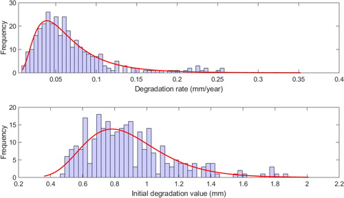
In order to test the lognormality of the degradation parameters, the Anderson-Darling (AD) test was applied. The p-values for the AD tests performed on the initial degradation value and degradation rate are 0.35 and 0.14, respectively. Considering the significance level of 0.05, the results of the tests show that there is no reason to reject the lognormality assumption for the initial degradation value and degradation rate. The estimated parameters of the lognormal distributions for the initial degradation value and degradation rate are presented in Table 3.

Table 3. The results of parameter estimation for lognormal distributions.

	Location parameters	Scale parameter
Initial degradation value	−0.17	0.26
Degradation rate	−2.77	0.61

To construct the tamping recovery model, the following explanatory variables were included: (1)$\mathrm{}{D}_s\left(t_{m_{i,s}}\right),$ which is the degradation level before a tamping intervention, (2)$\mathrm{}{x}_{1\mathrm{j},s},$ which is a dummy variable with value $0$ when the ${\mathrm{j}}^{\mathrm{th}}\mathrm{}$ tamping is a partial tamping performed on section $s$ and value $1$ when the ${\mathrm{j}}^{\mathrm{th}}\mathrm{}$ tamping is a complete tamping performed on section $s,$ and (3)$\mathrm{}{x}_{2,j,s}^{(2)},$$\mathrm{}{x}_{2,j,s}^{(3)},$ $x_{2,j,s}^{(4)},\mathrm{}{\mathrm{and}\mathrm{}x}_{2,j,s}^{(5)},$ which are dummy variables representing the second, third, fourth, and fifth interventions, respectively. The recovery model is formulated as follows: (7) $$R_{i,s}=a_1+b_0{D}_s\left(t_{m_{i,s}}\right)+b_1{x}_{1,j,s}+b_2{x}_{2,j,s}^{\left(2\right)}+b_3{x}_{2,j,s}^{\left(3\right)}+b_4{x}_{2,j,s}^{\left(4\right)}+b_5{x}_{2,j,s}^{\left(5\right)}+\mathrm{\delta }$$(7) where $a_1,\mathrm{}{b}_0,$ $b_1,$ $b_2,$ $b_3,\mathrm{}{b}_4,$ and$\mathrm{}{b}_5$ are the model coefficients. The estimated parameters of the recovery model obtained using the least squares algorithm are presented in Table 4.

Table 4. Parameter estimates for recovery model.

Parameter	$a_1$	$b_0$	$b_1$	$b_2$	$b_3$	$b_4$	$b_5$	${\mathrm{\tau }}^2$
Estimates	1.08	0.32	0.36	−0.13	−0.23	−0.30	−0.36	0.06

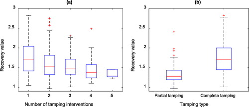
In order to illustrate the effect of the tamping type and the number of accumulated tamping interventions on the recovery value after tamping, two box plots were created, as presented in Figure 5. Figure 5a shows that the recovery value after tamping decreases as the number of tamping interventions increases, while Figure 5b displays that the expected recovery values after complete tamping interventions are higher than the expected recovery values after partial tamping.

Figure 5. (a) Box plot of the recovery values for different numbers of tamping interventions, (b) Box plot of the recovery values for different tamping types.

In order to estimate the probability of the occurrence of UH2 defects and critical defects, the model presented in Equation (4)(4) $$\text{logit(}Y\le k)=g_k\left(x\right)=\log (\frac{P(Y\le k)}{1-P(Y\le k)})={\theta }_{\mathrm{k}}+c_1{x}_1+c_2{x}_2+\dots +c_n{x}_n,k=1,\dots ,K$$(4) is used. In this study, the response variable$Y$ took a value of 0 whenever there was no longitudinal level defect in the track section, a value of 1 whenever there was at least one UH2 defect in the track section, and a value of 2 whenever there was at least one critical defect in the track section. The explanatory variable considered in the model is the standard deviation of the longitudinal level. The ordinal logistic regression for the proposed model is presented as follows: (8) $$P\left(Y\le k|x\right)=\frac{e^{{\theta }_{\mathrm{k}}+c_{1}S\mathit{DLL}}}{1+e^{{\theta }_{\mathrm{k}}+c_{1}S\mathit{DLL}}}$$(8) where $\mathit{SDLL}$ is the standard deviation of the longitudinal level. The results for the fitting of the model are summarized in Table 5.

Table 5. The ordinal logistic regression results for the longitudinal level defects.

	${\theta }_1$	${\theta }_2$	SDLL
P-value	<0.05	<0.05	<0.05
Coefficient$$	9.8	13.02	−5.02

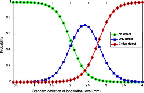
As can be seen in Table 5, the p-values of the standard deviation of the longitudinal level are less than the significance level. Therefore, it can be concluded that these variables have a significant effect on the probability of the occurrence of UH2 defects and critical defects. According to Table 5, the standard deviation of the longitudinal level has a negative coefficient. This means that the higher the standard deviation is, the higher is the probability of the occurrence of at least a UH2 defect or a critical defect. Figure 6 depicts the relationship between the standard deviation of the longitudinal level and the probability of the occurrence of UH2 defects and critical defects. As can be seen in Figure 6, when the standard deviation of the longitudinal level increases, the probability that a track section does not have a UH2 defect or critical defect decreases. As is obvious from Figure 6, increasing the standard deviation of the longitudinal level increases the probability of the occurrence of at least one critical defect in a track section.

Figure 6. Relationship between the standard deviation of the longitudinal level and the probability of no defect, at least one UH2 defect, and at least one critical defect in a track section.

5.2. Simulation results

By considering the longitudinal level as geometry parameters and using the proposed model, the percentage of time spent in different longitudinal level states can be estimated for the purpose of comparing different inspection intervals. In total, the effect of the following five different inspection intervals on the track longitudinal level has been assessed: 1 month, 2 months, 3 months, 4 months, and 6 months. The Monte Carlo simulation technique was used to obtain the expected values for the percentage of time spent in different longitudinal level states. The simulations were run for a 10-year period. The maintenance planning time for the performance of normal CM was assumed to follow a normal distribution with a mean of $m=5$ weeks and a standard deviation of $\sigma =1$ week. In order to perform PM, the tamping windows were set to be available every 18 months. The alert limit was considered to be 1.5 mm. For each simulation, 80,000 runs were performed to make sure that the simulation would be converged. Table 6 shows the percentage of time spent in the three defined longitudinal level states for different inspection intervals.

Table 6. Effect of the inspection interval on the percentage of time spent in the different longitudinal level states.

Inspection interval	State 1	State 2	State 3
1 Month	99.26%	0.69%	0.05%
2 Months	98.55%	1.35%	0.10%
3 Months	97.85%	2.01%	0.14%
4 Months	97.20%	2.62%	0.18%
6 Months	95.79%	3.91%	0.30%

It must be noted that the running behaviour of the train is influenced by the amplitude of the track irregularities. Therefore, the percentage of time that track sections spend in different longitudinal level states has a significant effect on the level of safety and the ride comfort. If the track longitudinal level degrades to state 2 and state 3, this will negatively affect the energy consumption, the degradation rate of other track components, and passenger satisfaction. From an availability point of view, the number of speed restrictions that a track section suffers in a given period of time is related to the track geometry state. In fact, when the track longitudinal level degrades to state 2 and state 3, there is a higher probability of the occurrence of temporary speed restrictions. From a safety point of view, the risk of derailment in a given track section is dependent on the number of isolated defects, the amplitude of those defects, and the length of the time during which those defects are not detected. Therefore, if the percentage of time spent in state 3 increases, the risk of train derailment increases.

The results of the Monte Carlo simulation show that the inspection frequency has a significant effect on the time that a track section spends in different longitudinal level states. Based on the results obtained, changing the inspection interval from one month to six months increases the percentage of time that a track section spends in state 2 and state 3 by 3.22% and 0.25%, respectively. According to Table 6, the shorter the inspection interval is, the shorter is the length of time spent by a track section in state 2. In addition, as the results of the simulations indicate, decreasing the frequency of inspections will significantly increase the percentage of time spent in state 3. When the length of the inspection interval increases, UH2 defects will be detected later. Therefore, with longer inspection intervals there is a higher probability that a UH2 defect will turn into a critical defect.

6. Conclusions

The aim of the research presented in this paper has been to develop an integrated approach to investigation of the effect of different inspection intervals on the track geometry condition. The standard deviation of the longitudinal level and the extreme values of isolated defects of the longitudinal level were considered as quality indicators to assess the need for PM and CM activities, respectively. The developed approach involves the use of a random coefficient piecewise exponential model to characterize the track geometry degradation and restoration. In addition, ordinal logistic regression is used to estimate the probability of the occurrence of isolated defects. The proposed model can be used to make predictions of the percentage of time that a track section will spend in the different track geometry states in a given time horizon.

Such predictions are very important, as they are a primary input for predicting the probability of the occurrence of temporary speed reductions and the risk of derailment. To verify the applicability of the proposed approach, a case study has been conducted using a data set collected from the Main Western Line in Sweden. Based on the results obtained, it was observed that varying the length of the inspection intervals has a significant effect on the percentage of time spent by the track in different longitudinal level states. It must be noted that the proposed approach can also be used to predict the number of different maintenance actions, i.e., PM, normal CM, and emergency CM.

However, since in the present study it is assumed that the PM actions are carried out on the track at predetermined times, the number of PM actions and normal CM actions is not sensitive to different inspection intervals. In the case of a condition-based maintenance policy being implemented, the inspection frequency may affect the number of PM actions and normal CM actions. In this case, by determining the different direct and indirect costs for preventive tamping actions, normal corrective tamping actions, emergency corrective tamping actions, inspection, derailment, and the loss of capacity, the life cycle cost of each inspection interval can be assessed for the purpose of choosing the most effective one.

Acknowledgements

The authors would like to thank Trafikverket, Bana Väg För Framtiden (BVFF), Luleå Railway Research Center (JVTC), and SIMTRACK project partners for their technical and financial support provided during this project.

Disclosure statement

No potential conflict of interest was reported by the authors.

References

- Albisua, I., Arbelaitz, O., Gurrutxaga, I., Lasarguren, A., Muguerza, J., & Pérez, J. M. (2013). The quest for the optimal class distribution: an approach for enhancing the effectiveness of learning via resampling methods for imbalanced data sets. Progress in Artificial Intelligence, 2(1), 45–63. doi:10.1007/s13748-012-0034-6
- Andrade, A. R., & Teixeira, P. F. (2013). Unplanned-maintenance needs related to rail track geometry. Proceedings of the Institution of Civil Engineers - Transport, 167(6), 400–410. doi:10.1680/tran.11.00060
- Andrews, J., Prescott, D., & De Rozières, F. (2014). A stochastic model for railway track asset management. Reliability Engineering & System Safety, 130, 76–84. doi:10.1016/j.ress.2014.04.021
- Arasteh Khouy, I., Larsson-Kråik, P., Nissen, A., Juntti, U., & Schunnesson, H. (2014). Optimisation of track geometry inspection interval. Proceedings of the Institution of Mechanical Engineers, Part F: Journal of Rail and Rapid Transit, 228(5), 546–556.
- AREMA. (2006). Manual for railway engineering (Report No. 4). American Railway Engineering and Maintenance-of-Way Association USA.
- Cárdenas-Gallo, I., Sarmiento, C. A., Morales, G. A., Bolivar, M. A., & Akhavan-Tabatabaei, R. (2017). An ensemble classifier to predict track geometry degradation. Reliability Engineering & System Safety, 161, 53–60.
- EN 13848–5. (2008). Railway applications – track – track geometry quality – Part 5: Geometric quality levels. Brussels, Belgium: CEN (European Committee for Standardization).
- Haixiang, G., Yijing, L., Shang, J., Mingyun, G., Yuanyue, H., & Bing, G. (2017). Learning from class-imbalanced data: review of methods and applications. Expert Systems with Applications, 73, 220–239.
- He, H., Bai, Y., Garcia, E. A., & Li, S. (2008). ADASYN: adaptive synthetic sampling approach for imbalanced learning. Paper presented at 2008 IEEE International Joint Conference on Neural Networks (IEEE World Congress on Computational Intelligence), Hong Kong, China.
- Hosmer, D. W., Jr, Lemeshow, S., & Sturdivant, R. X. (2013). Applied logistic regression. Hoboken: John Wiley & Sons.
- Loyola-González, O., Martínez-Trinidad, J. F., Carrasco-Ochoa, J. A., & García-Borroto, M. (2016). Study of the impact of resampling methods for contrast pattern based classifiers in imbalanced databases. Neurocomputing, 175, 935–947.
- Lyngby, N., Hokstad, P., & Vatn, J. (2008). RAMS management of railway tracks. In Handbook of performability engineering (pp. 1123–1145). London: Springer.
- Meier-Hirmer, C., Sourget, F., & Roussignol, M. (2005). Optimising the strategy of track maintenance. Paper presented at Advances in Safety and Reliability, proceedings of ESREL 2005-European Safety and Reliability Conference 2005, Tri City (Gdynia–Sopot–Gdańsk), Poland.
- Osman, M. H. B., Kaewunruen, S., Jack, A., & Sussman, J. (2016). Need and opportunities for a ‘Plan B’ in rail track inspection schedules. Procedia Engineering, 161, 264–268.
- Quiroga, L. M., & Schnieder, E. (2012). Monte Carlo simulation of railway track geometry deterioration and restoration. Proceedings of the Institution of Mechanical Engineers, Part O: Journal of Risk and Reliability, 226(3), 274–282. doi:10.1177/1748006X11418422
- Soleimanmeigouni, I., Ahmadi, A., & Kumar, U. (2018). Track geometry degradation and maintenance modelling: a review. Proceedings of the Institution of Mechanical Engineers, Part F: Journal of Rail and Rapid Transit, 232(1), 73–102.
- Soleimanmeigouni, I., Ahmadi, A., Letot, C., Nissen, A., & Kumar, U. (2016). Cost-based optimization of track geometry inspection. Paper presented at 11th World Congress of Railway Research, Milan, Italy.
- Soleimanmeigouni, I., Xiao, X., Ahmadi, A., Xie, M., Nissen, A., & Kumar, U. (2018). Modelling the evolution of ballasted railway track geometry by a two-level piecewise model. Structure and Infrastructure Engineering, 14(1), 33–45.
- SS-EN 13848-1: 2004 + A1. (2008). Railway applications – track – track geometry quality –Part 1 Characterisation of track geometry. Sweden: Swedish Standard Institute.
- Sun, Y., Kamel, M. S., Wong, A. K., & Wang, Y. (2007). Cost-sensitive boosting for classification of imbalanced data. Pattern Recognition, 40(12), 3358–3378.
- Trafikverket. (2015). Banöverbyggnad – Spårläge – Krav vid Byggande och Underhåll (Track superstructure – Track geometry – Requirements after renewal and maintenance, in Swedish). TDOK 2013:0347 v3.0. Borlänge, Sweden: Trafikverket.
- UIC. (2008). Best practice guide for optimum track geomerty durability. Paris, France: ETF - Railway Technical Publications.
- Zaayman, L. (2017). The basic principles of mechanized track maintenance (3rd ed.). Bingen am Rhein: PMC Media House. doi:978-3-96245-151-6.