Variable mass loading effect on the long-term ambient response of a freeway bridge

Abstract

This study addresses the quantification and compensation of the so-called mass loading effect, a disturbance that typically occurs in structural health monitoring of bridges. Source of this effect is the time-variant traffic, which means that dynamic performance indicators such as identified resonance frequencies are also time-variant. Basis of this study is the ambient acceleration response of a freeway bridge in the Alps recorded in a long-term monitoring campaign. After statistical evaluation of the traffic over the bridge, stochastic finite element simulations are performed to quantify the effect of time-variant truck traffic on a resonance frequency identified from the recorded accelerations, which serves as performance indicator. The corresponding natural frequency of the numerical bridge-truck model is obtained both by modal analyses and response history analyses, whose results however show considerable differences. In an effort to reduce the temporal scatter of the performance indicator, the corresponding natural frequency of the numerical model is used to compensate for the mass loading effect. It it shown that the mass loading effect plays a significant role for the considered bridge, although temperature effects dominate as a disturbance for the identified resonance frequency.

KEYWORDS:

• Structural health monitoring
• ambient response
• long-term measurement
• system identification
• mass loading
• truck traffic
• bridge dynamics

1. Introduction

In the last decades, Structural Health Monitoring (SHM) has become a highly regarded topic in structural engineering (Sohn et al., 2004). This is due to the facts that an increasing part of infrastructure is at an advanced age and that loading assumptions made during construction are no longer valid. The latter applies in particular to bridges where traffic volume has significantly increased over the years (Wenzel & Veit-Egerer, 2011), (Ivanković, Skokandić, Žnidarič, & Kreslin, 2019). Therefore a periodical or continuous assessment of the bridge condition is required.

A large number of SHM methods use vibration-based kinematic quantities (strains, deformations, velocities, accelerations) in both research and engineering practice to monitor the structure under consideration. Since bridge structures are dynamically excited by nature through traffic loads, wind and microseismicity, these response variables can be measured without artificial excitation, which is difficult to realize in practice due to the large forces and logistics required. In operational modal analysis (OMA) it is assumed that the dynamic excitation can be mathematically modeled by a white-noise random process (Brincker & Ventura, 2015; Rainieri & Fabbrocino, 2014), which is characterized by a constant amplitude power spectral density (PSD). Thus, by measuring the structural response at a number of points, a transfer function matrix of the system can be derived. From this transfer function matrix, the modal parameters (resonance frequencies, damping ratios and mode shapes) are identified. Once a performance indicator has been chosen (either one of the modal parameters or a post-processing variable such as the mode shape curvature (Pandey, Biswas, & Samman, 1995) or the normalized cumulative PSD (Tributsch & Adam, 2018)), in theory a change in this indicator value is associated with a change in system stiffness, which in many cases indicates deterioration or damage to the structure.

In reality, however, various disturbance effects can lead to changes in the performance indicators regardless of structural damage. Environmental conditions, particularly temperature, are considered to be the most important disturbance effect occurring (Sohn, 2007). Consequently, a number of studies are dealing with the influence of temperature on modal properties, see for instance Peeters and Roeck (2001) and Moser and Moaveni (2011).

Another disturbance effect, especially for bridges, is due to the temporal variability of traffic loads. Traffic loads violate the assumption of stationarity on which OMA is based. This problem is addressed by sufficient averaging to minimize random errors (Brandt, 2011). Moreover, vehicles and bridge represent an interacting time-variant oscillating system. Thus, each identified modal parameter corresponds to the coupled interacting system, but not to the bridge. The most obvious effect of crossing vehicles is the addition of mass to the bridge; therefore the term mass loading effect has become established in the literature (Sohn, 2007).

Several authors have addressed the mass loading effect from different perspectives. For instance, in (Kim, Jung, Kim, & Yoon, 1999), based on experiments on a short-span bridge, differences in the resonance frequencies between the crossing of heavy and light trucks of up to 5.4% are reported, whereas no differences were observed on a three-span suspension bridge. Similar results are presented in (Roeck, Maeck, Michielson, & Seynaeve, 2002), but on the basis of a numerical study on a simply supported beam crossed by a moving lumped mass and three different vibratory systems representing quarter-car models, respectively. According to this study, an upper limit for the mass loading effect can be estimated by a modal analysis of the beam with the lumped mass located at the most critical location. Another experimental study (Zhang, Fan, & Yuan, 2002) shows an increase in the identified modal damping ratios as soon as a certain acceleration level reflecting a certain amount of traffic loads is reached. In González, Rattigan, OBrien, and Caprani (2008), static loading conditions representing critical dynamic loading events were investigated and dynamic amplification factors derived. It is shown that a detailed finite element (FE) analysis considering vehicle-bridge interaction delivers lower dynamic amplification factors than those provided in the codes, thus allowing for a more economical bridge design.

In Westgate, Koo, and Brownjohn (2015), both temperature and mass loading effects are treated for a suspension bridge. Some foundations of this study are the hourly statistics of different vehicle classes and the diurnal variation of different resonance frequencies determined from vibration measurements. The results of analyses on an FE model of the structure with attached lumped masses representing the vehicles were used to derive linear regression models to predict the resonance frequency variation due to the additional mass. For the same bridge, a principal component analysis of the identified resonance frequency data was used in Cross, Koo, Brownjohn, and Worden (2013) to separate the effects of temperature, traffic loading and wind speed. Both temperature and traffic loading were found to have significant, separable influences on the frequency variation. One of the key results of this study is a response surface model based on a linear relationship between traffic load and resonance frequency, which allows a good fit to experimentally obtained data. This approach has recently been extended in Worden and Cross (2018) by enabling a switch between the models using treed Gaussian processes. Significant improvements were achieved in the detection the temperature effect on the resonance frequencies when the temperature falls below the freezing point.

In Sheibani, Hadjian-Shahri, and Ghorbani-Tanha (2017), the mass loading due to time-variant traffic is quantified for a simply-supported beam bridge with respect to the mass scaling of the mode shapes, considering the mass loading as a perturbation of the mass matrix. In another numerical study (Yang, Lin, & Yau, 2004), the vehicle is modeled as a single-degree-of-freedom (SDOF) oscillator, which crosses a simply-supported beam bridge. It is shown that in the acceleration spectrum of the bridge response the original bridge frequency (without vehicles) is shifted by an amount of $\pm \pi v/L,$ with v denoting the speed of the vehicle and L the bridge span. The temporal variation of bridge frequencies and modes shapes of a bridge induced by a truck with constant speed was investigated both experimentally and numerically in Cantero, Hester, and Brownjohn (2017). Both an increase and decrease of the natural frequencies of the coupled bridge-vehicle system compared to the corresponding uncoupled bridge frequencies could be observed. As already noted by other authors, it has been found that the interaction effects are most pronounced when the mass ratio between vehicle and bridge is high.

Recently, non-modal vibration parameters are gaining popularity in SHM. In Delgadillo and Casas (2020), several empirical vibration parameters are compared in view of damage detection for bridges. For vehicle-induced vibrations, the instantaneous vibration intensity turned out as promising parameter. Basis of this parameter is an empirical mode decomposition (EMD) of acceleration signals. A subsequent Hilbert-Huang transform yields instantaneous amplitudes and phases, which are combined to form a vibration intensity measure. It is found that this intensity can serve as a damage indicator when comparing typical damage scenarios under a well-defined loading. The reason for using EMD is that vehicles passing the bridge yield non-stationary vibration signals. This issue is also addressed in Martin-Sanz et al. (2020) where time-dependent auto-regressive models are used to model this non-stationarity. Compared to a standard spectrogram based on a short-time Fourier transform, the considered model offers a highly improved frequency resolution.

With regard to these contributions, the present paper aims to combine these approaches to identify and quantify the mass-loading effect on SHM data. One basis of this study is the acceleration response of a freeway bridge, which is part of a main traffic route through the European Alps, recorded in a long-term monitoring campaign. This is presented in Section 2. The evaluation of this response provides a resonance frequency and its temporal variation over a period of five years, as will be shown in Section 3. In Section 4, the traffic over the bridge is quantified by a detailed statistical evaluation of the traffic volume, resulting in probability distributions on an hourly basis. Based on these data and a numerical model of the bridge-vehicle system presented in Section 5, the mass loading effect on the identified resonance frequency is evaluated by stochastic FE simulations in Section 6, performing both modal analysis and response history analysis. In Section 7, these simulation results are utilized to compensate the mass-loading effect. The paper ends with conclusions in Section 8.

2. Long-term monitoring of the considered bridge

The considered Lueg bridge, completed in 1969, is located near the Brenner Pass and carries the Austrian section of the four-lane Brenner freeway A13 along a mountain slope connecting Austria and Italy (see Figure 1). The bridge with a total length of $1800 m$ consists of five segments of approximately equal length. Each segment is a multiple supported continuous girder system with a standard span of about $36 m.$ Four segments are made of prestressed concrete, while the cross-section of one segment consists of a steel truss and a reinforced concrete slab. In this segment the standard span width is $72 m.$

Figure 1. Aerial photograph of the Lueg bridge (Brenner Autobahn AG, 1972).

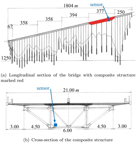
In a long-term monitoring campaign, which was carried out within the framework of a funded research project (Veit-Egerer, Widmann, & Wenzel, 2008), the company VCE Vienna Consulting Engineers ZT GmbH recorded from December 2006 to September 2011 the ambient bridge accelerations continuously at a sample rate of $100 Hz.$ From the acceleration signals obtained with a triaxial force-balance accelerometer of type Kinemetrics FBA 23 attached to the steel truss of the composite bridge segment, a characteristic resonance frequency is identified in the present study, which serves as a performance indicator of the bridge. Figure 2 shows the sensor position in the longitudinal section and the cross-section of the bridge. The sensor was placed outside the center of the cross-section to capture possible torsional vibrations more clearly. It should be noted that in the framework of the project, two more acceleration sensors and two dilatation sensors were attached to the prestressed concrete segments. However, this part of the bridge is out of the scope of the present investigation.

Figure 2. Longitudinal and cross-section of the Lueg bridge (Brenner Autobahn AG, 1972), acceleration sensor location marked.

The Brenner Pass is a major mountain pass between Austria and Italy, and therefore the Brenner freeway is one of the most important transit routes between Northern and Southern Europe for both freight and holiday traffic. Thus, the application of vibration based SHM on this bridge requires the quantification of the mass-loading effect on the considered performance indicator. Figure 3 shows the total number of vehicles passing the bridge per day in 2008. As observed, the traffic volume is higher during the holiday periods, with peaks on Saturdays throughout the year.

Figure 3. Number of all crossing vehicles and trucks per day recorded near the Lueg bridge in 2008.

In Veit-Egerer (2014), the number of trucks (i.e. vehicles with a mass of more than $8.7 t$) crossing the Europa bridge, which is also part of the Brenner freeway, is specified for this observation period. It is realistic to assume that the Lueg bridge carries the same trucks, since the Europa bridge is only $25 km$ north with no major exit in-between. In Figure 3, red circular markers indicate the number of trucks counted per day, except for the period from mid of May to the end of June, for which no data are available. In contrast to the overall traffic volume, daily truck traffic from Monday to Saturday is relatively constant throughout the year, with an average of around 6000 trucks per day. On Sundays and holidays, however, due to the ban on truck traffic in Austria from Saturday 3 p.m. to Sunday 10 p.m. and on holidays from midnight to 10 p.m., a significant decline in heavy goods traffic can be observed. This ban also applies every night from 10 p.m. to 5 a.m.

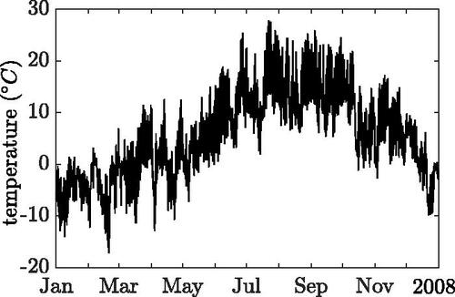
As outlined in the introduction, additionally to the mass loading effect due to the traffic, another difficulty in evaluating the ambient vibration response arises from large temperature fluctuations. Since it is located at an altitude of about $1300 m,$ the Lueg bridge is exposed to pronounced seasonal climatic changes. The annual ambient temperature profile shown in Figure 4, recorded at the weather station of the nearby Brenner Pass in 2008, shows that the temperature varies over the course of a year in a range from $-{20}^{°}C$ to ${30}^{°}C,$ and that there is frost during half of the year. Therefore, a performance indicator of the Lueg bridge based on recorded vibration data is affected by the environmental temperature. However, the assessment, quantification and compensation of this effect is not subject of this study.

Figure 4. Daily ambient mean temperature recorded near the Lueg bridge in 2008.

3. System identification

3.1. Measurement data analysis

To identify the characteristic bridge resonance frequency, first the power spectral densities (PSDs) of the recorded time-histories of the bridge acceleration are estimated by Welch’s estimator (Welch, 1967). Decisive for the PSD estimation is an appropriate choice of the data length and the number of averages. In Brandt (2011), the respective bias and random errors are discussed in detail. For example, if a resonance frequency $f_r=2 Hz$ and a corresponding damping ratio of ${\zeta }_r=0.01$ is to be estimated with a normalized bias error of less than 1%, the frequency resolution should be less than $0.0036 Hz.$ On the other hand, if 100 data segments with an overlap 50% and a Hanning window are used, the normalized random error is still 10%. This error can be somewhat reduced by using segments with an overlap of $60-65\%$ as shown in Nuttall and Carter (1982). For a target frequency resolution of $0.0025 Hz$ with an overlap of 64% between the data segments, the measurement period must be $14,400 s.$ Therefore, the PSDs are estimated here with a data length of $14,400 s=4 h.$ Subsequent PSDs are computed with an overlap of 75%, which corresponds to a PSD update period of $1 h.$ For the PSD to be valid, the underlying signals have to be stationary. Therefore, stationarity tests as implemented in the Econometrics Toolbox in MATLAB were performed for a sample acceleration time-history of one day. With the chosen segment length of $4 h,$ all of the tests (Augmented Dickey-Fuller, Leybourne-McCabe, Kwiatkowski-Phillips-Schmidt-Shin and Phillips-Perron) confirmed the null hypothesis that the data is stationary for all segments.

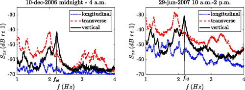
As an example, Figure 5 shows in logarithmic scale the resulting auto PSDs, S_xx, of the three orthogonal acceleration components recorded at two different seasons. The underlying signals of the left plot were recorded in winter at night (10 December 2006) from midnight to 4 a.m., the PSDs of the right plot are based on accelerations measured during summer at noon (29 June 2007) from 10 a.m. to 2 p.m. As observed, the longitudinal vibrations are orders of magnitude smaller than in the other directions and are therefore not considered further. The PSDs of the transverse and vertical vibration components are of the same order of magnitude and show several distinct resonance peaks in the frequency range from 1 to $4 Hz.$ The bridge is supported by long piers of up to $50 m$ (see Figure 1), and thus the recorded transverse response is mainly related to bending of the piers. Since the focus of this study is on the structural condition of the bridge deck, but not on the piers, the transverse response component is not discussed in detail.

Figure 5. Auto spectral density of the three acceleration components for two different periods of time.

3.2. Performance indicator

In the two sub-diagrams of Figure 5, the PSD of vertical acceleration at a frequency of about $2.2 Hz$ shows a well separated peak. This apparent resonance frequency is chosen as a performance indicator. Since only one sensor output is available, peak-picking is the obvious choice to identify the frequency at this peak from the PSDs at one-hour intervals during the entire observation time from December 2006 to September 2011.

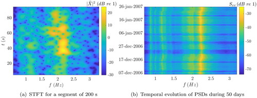
Figure 6 shows results of time-frequency analyses of the recorded acceleration signals $\ddot{x}.$ In Figure 6(a), results of a short-time Fourier transform (STFT) of a signal segment with $100 s$ duration is shown, based on $10 s$ segments. The number of trucks on the bridge during this period is unknown, however the Figure clearly demonstrates the non-stationarity of the acceleration signal on this time-scale. In fact, the Leybourne–McCabe and the Kwiatkowski–Phillips–Schmidt–Shin tests yield a rejection of the stationarity hypothesis. On a longer time-scale, Figure 6(b) depicts the temporal evolution of PSDs of the vertical acceleration component from 10 December 2006 to 26 January 2007, evaluated in $4 h$ time segments, as outlined in the previous section. The resonance frequency at approximately $2.2 Hz$ (yellow range) is clearly visible within the 50 day period, although PSD amplitude levels differ significantly. The horizontal blue ‘lines’ indicate low PSD values, which means that traffic is low during the corresponding period. This is a consequence of the aforementioned ban on heavy goods vehicles at nights, weekends and holidays, see for instance the period from 24 December to 26 December. However, not only the PSD values drop at those periods, but also a temporal variation of the resonance frequency in the vicinity of $2.2 Hz$ is observed.

Figure 6. Time-frequency analysis of acceleration signals.

Figure 7 shows this identified resonance frequency (referred to as f_id) for three time intervals of 50 consecutive days: Sub-diagram (a) represents data of the December–January period of three different winters, sub-diagram (b) refers to three periods of March–April, and sub-diagram (c) corresponds to the July–August period of three consecutive summers. This figure reveals that the frequency f_id varies over time in the range from $2.15 Hz$ (summer) to $2.35 Hz$ (winter). As no structural damage was observed during the entire monitoring period, it can be concluded that other effects are responsible for the frequency variability. As observed, during the cold season the mean of frequency f_id is greater, indicating the sensitivity of the system parameters to low temperatures. For instance, the subsoil under abutments, asphalt, etc. become stiffer at low temperatures due to ice formation. It is also observed that the frequency fluctuation is greater in winter than in summer, a consequence of freeze-thaw cycles in winter.

Figure 7. Variation of the identified resonance frequency in three 50 day periods of three subsequent years.

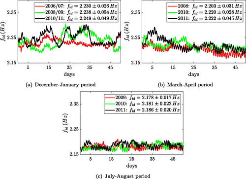
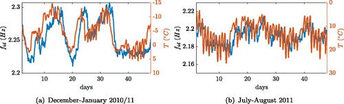
For the time intervals considered, the mean value ± twice the standard deviation σ of f_id is given in the legends of Figure 7. Assuming a normal distribution, the range $\pm 2\sigma$ approximates the 95% confidence interval of frequency, representing its uncertainty. This resonance frequency can only serve as a performance indicator if the effects of variable traffic and ambient temperature are compensated. That is, the temporal variation is eliminated or at least reduced, resulting in a significant decrease of the 95% confidence interval of the frequency f_id. In Figure 8, for two 50 days periods the identified resonance frequency is displayed in conjunction with the corresponding ambient temperature. Both in winter (Figure 8(a)) and in summer (Figure 8(b)) a strong correlation of these parameters is visible. In winter, the time delay between ambient temperature and resonance frequency seems to be more pronounced than in summer. In can be concluded that the influence of ambient temperature on the frequency is dominating, however this effect is not the subject of the current study. Here, the unknown effect and significance of variable mass loading will be assessed. Therefore, statistics on the traffic volume crossing the Lueg bridge are evaluated, which serve as the basis for stochastically generated load patterns describing the impact of trucks on a numerical bridge model.

Figure 8. Identified resonance frequency and ambient temperature in two 50 day periods.

4. Statistical evaluation of the traffic volume

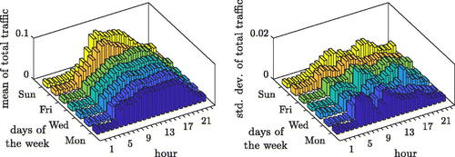
A basis for the assessment of the mass loading effect is the statistical evaluation of the traffic volume. Based on counted traffic data of the Europa bridge presented in Figure 3, the histogram of the daily variation of traffic over the bridge is determined for each day of the year of observation in form of one-hour intervals. Normalizing the total area of the histogram to one yields an approximation of the corresponding probability density function of daily traffic. Then, the normalized histograms of all Mondays (Tuesdays, Wednesdays, etc.) in the observation year 2008 are statistically analyzed. As the result of this analysis, Figure 9 shows the normalized histograms of the daily traffic volume in relation to its mean values and standard deviations. Holidays are treated like Sundays, i.e. the histogram of the Sunday also contains the traffic information of those holidays. Examination of Figure 9 confirms that most of the traffic crosses between 5 a.m. and 10 p.m. the bridge, which is partly due to the driving ban on heavy goods traffic beyond this period. It can also be observed that on weekdays the daily distribution of traffic is similar, but on Saturdays and Sundays the characteristics of traffic flow are different.

Figure 9. Daily distribution of total traffic volume with relation to the time of day.

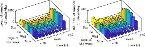
According to Figure 3, trucks account for about 20% of the total traffic volume. Considering that in Austria the gross vehicle mass of trucks is limited to 44 metric tons (t), which is one order of magnitude larger than the mass of passenger cars, it can be concluded that the mass added on the bridge is dominated by heavy goods traffic. In Veit-Egerer (2014), the mass of each truck crossing the Europa bridge in 2008 is specified, and the trucks are divided into nine mass classes: Mass class 1 (8.7–10t) includes vehicles carrying little to no load, while mass class 9 (40–44t) includes the fully loaded trucks. Figure 10 shows for each mass class the mean values and standard deviations of the truck number of each weekday, evaluated over the observation period 2008. Holidays are treated as Sundays as before. It is readily observed that most of the trucks belong to the mass classes 1 and 9. From Monday to Saturday the number of unloaded trucks is almost stationary, while on Sundays the number of fully loaded trucks is much lower compared to the other six days of the week. Despite the traffic ban, heavy goods traffic at the weekends is still considerable due to special permits.

Figure 10. Daily quantity of trucks as a function of vehicle mass.

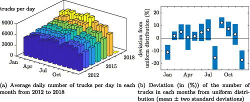
From the publicly available traffic statistics (ASFINAG, 2019), the average number of trucks at a nearby counting point is available for each month from January 2012. Two conclusions can be drawn from the data presented in Figure 11(a): (i) truck traffic is increasing steadily over the years, and (ii) within each year, the amount of truck traffic shows significant monthly fluctuations. To better illustrate the latter fact, monthly data from Figure 11(a) are normalized by the total number of trucks for each year. Then the mean and standard deviation of the monthly share of the traffic volume for each month is calculated. If truck traffic were evenly distributed within a year, this ratio would be 1/12. In Figure 11(b), deviations from this value are represented by a range of mean value ± two standard deviations for each month. In January, August and December, the amount of truck traffic is significantly lower by $10-20\%$ on average, while in September it is higher by 10% on average. From this discussion it becomes clear that the traffic volume over the Lueg bridge is highly non-stationary.

Figure 11. Statistics on the daily quantity of trucks as a function of month.

5. Modeling, simulation and evaluation strategy

5.1. Bridge model

To quantify the influence of the truck traffic on the resonance frequency in the vicinity of $2.2 Hz,$ an FE model of the considered bridge segment of the Lueg bridge is created. In this model, the structure is discretized by means of beam elements, which allows an efficient stochastic analysis of the response caused by the large number of moving vehicles.

In a step preceding the analysis of the dynamic response, the stiffness parameters of the beam elements are derived on the basis of another FE model of a representative cross-section segment between two cross girders, whose dimensions are found in (Brenner Autobahn AG, 1972). The concrete deck is modeled with solid elements, main girders and subgirders in longitudinal direction are modeled with shell elements and transverse bracing members with beam elements, as shown in Figure 12(a). To the cross-section segment unit displacements and rotations are imposed by constraining all nodes of the two intersection planes by one control node each. The evaluation of the induced reaction forces and moments yields the equivalent beam stiffness parameters given in Table 1. As an example, Figure 12(b) shows the cross-sectional displacement due to uniaxial bending. The mass per unit length of this FE model is $\rho A=20.4 t/m.$ To take into account non-structural masses not included in the FE model, in the following simulations with the beam model $\rho A=23 t/m$ is used.

Figure 12. FE simulation for derivation of equivalent beam stiffness parameters.

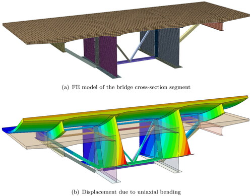
Table 1. Equivalent beam stiffness parameters for unit deformations of the bridge cross-section segment.

Torsional stiffness	GIt	=	$1.48·{10}^{11} N{m}^2$
Bending stiffness (vertical axis)	EIy	=	$8.51·{10}^{12} N{m}^2$
Bending stiffness (horizontal axis)	EIz	=	$4.35·{10}^{11} N{m}^2$
Transverse shear stiffness (vertical axis)	GAy	=	$1.12·{10}^{10} N$
Transverse shear stiffness (horizontal axis)	GAz	=	$7.41·{10}^{10} N$

In preliminary test calculations on a 3D beam model with these stiffness properties it was found that torsional modes are irrelevant in the considered frequency range ($2-2.5 Hz$). Therefore, the FE model of the bridge implemented in MATLAB consists of 2D Timoshenko beam elements. This beam model shown in Figure 13 rests on elastic springs which represent the axial flexibility of the supporting piers and the subsoil. Based on information available in (Brenner Autobahn AG, 1972), an axial stiffness of the piers $k_1=EA/l_p=30·{10}^8 N/m$ is obtained, taking into account a cross-section area $A=5 m^2,$ pier length $l_p=50 m$ and Young’s modulus $E=30·{10}^9 N/m^2.$ For the subsoil, according to Wolf (1994) $k_2=4Gr/1-\nu =6·{10}^8 N/m$ is obtained, based on a shear modulus of the subsoil $G=15·{10}^6 N/m^2,$ foundation radius $r=6 m$ and Poisson’s ratio $\nu =0.4.$ Connecting the springs in series yields $k={(1/k_1+1/k_2)}^{-1}=5·{10}^8 N/m.$ At the beginning and end of the model, there are also axial springs with the stiffness k to approximate the elastic connection of the considered composite bridge with the adjacent prestressed concrete bridge segments. In Figure 13, the position of the sensor measuring acceleration ${\ddot{u}}_{\mathit{mon}}$ (compare Figure 2) is shown. The first six natural frequencies of the bridge model without trucks are given in Table 2 and the corresponding mode shapes shown in Figure 14.

Figure 13. Mechanical model of the bridge with truck crossing and location of the acceleration sensor.

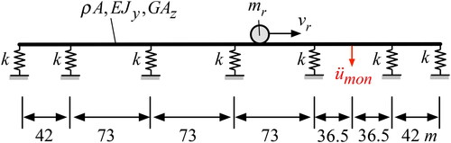
Figure 14. Mode shapes for natural frequencies f₂, f₄ and f₆ of the FE model using 2D beam elements.

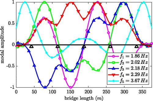
Table 2. Natural frequencies and participation factors for the first five modes of the 2D FE model.

Mode no. I	1	2	3	4	5
Natural frequency fi (Hz)	1.85	2.01	2.18	2.29	3.66
Participation factor Li	0.00	0.26	0.00	1.06	0.54

In order to uncover the most important mode for traffic loading, for each mode the participation factor (Clough & Penzien, 2003)(1) $$L_i={\int }_0^l{\psi }_i(x)dx, i=1,\dots ,6$$(1) is determined, where ψ_i is the ith mass-normalized mode shape and l denotes the total bridge length. This definition of the participation factor implies a line load equally distributed over the bridge as excitation, which corresponds to a convoy of equal trucks. As can be seen from the values given in Table 2, only modes 2, 4 and 5 have non-negligible participation factors. The participation factors of modes 1 and 3 are zero because the corresponding mode shapes are odd, as can be seen in Figure 14, i.e. ${\int }_0^l{\psi }_i(x)dx=0,$ i = 1, 3. Since mode 2 has a significantly lower participation factor than modes 4 and 5, it will not be considered further in the following. In mode 5 with frequency $f_5=3.66 Hz$ the largest modal displacements occur at the two end spans, while they are comparatively small in the four main spans. The remaining 4th mode has a mode shape with pronounced modal displacements over the four inner bridge spans. Therefore, a series of trucks crossing the bridge excites this mode continuously from the first to the last modeled column. Comparing the corresponding natural frequency $f_4=2.29 Hz$ with the dominating frequency f_id previously identified from the recorded ambient accelerations (see Figures 6 and 7) shows that also the response of the actual bridge is dominated by this mode. Consequently, in the subsequent numerical simulations special emphasis is placed on mode 4.

5.2. Mechanical truck model

The basic dynamic properties of a truck can be captured with a model in the form of a multi-body system composed of rigid bodies with mass connected by springs and dashpot dampers. As an example, in (Simeon, Grupp, Führer, & Rentrop, 1994) a planar model for a $18 t$ truck is presented. In a simpler approach, the vehicle is represented by a series of modal SDOF oscillators, as examined in Cantero et al. (2017). However, the spring force of the vehicle suspension is typically nonlinear, and consequently an appropriate linearized spring stiffness, which strongly depends on the truck type and the load, must be determined (Simeon et al., 1994). The literature on the dynamic properties of trucks is quite scarce, and particularly for the entire ensemble of vehicles encountered in practice no studies have been published to the best of the authors’ knowledge. Since the Lueg bridge was crossed by a large number of vehicles of different types with unknown parameters (spring stiffnesses, damping ratios, mass distributions) during the observation period, the dynamic vehicle characteristics cannot be taken into account in the present study on the global impact of the mass loading effect on the structure. Therefore, in the following simulations the rth truck is represented as a lumped mass m_r crossing the bridge model at the constant speed v_r, see Figure 13. The horizontally moving truck model is rigidly coupled vertically to the structural beam model.

5.3. Stochastic model for truck traffic

For the truck traffic crossing the bridge model, a stochastic model is built using several random variables. Basis of this stochastic model is the statistically evaluated data of the counted traffic for each day of the week, as described in Section 4. The number of trucks in each mass class is assumed to be a standard-normally distributed random variable with the mean value and standard deviation according to Figure 10. These random variables are accumulated in the vector ${\mathbf{y}}_1\in {\mathbb{R}}^9\sim \mathcal{N}(0,1).$ The random vector ${\mathbf{y}}_2\in {\mathbb{R}}^{24}\sim \mathcal{N}(0,1)$ contains the set of 24 standard normally distributed random variables that describe the distribution of the heavy traffic at one-hour intervals during the course of the day. The mean and standard deviation of these variables can be read from Figure 9. The actual mass of a truck within a mass class is captured by another uniformly distributed random variable denoted as ${\mathbf{y}}_3.$ It is assumed that the trucks cross the bridge at constant but random speed (denoted as y₄) with a mean value of $50 km/h$ and a standard deviation of $10 km/h.$ Another assumption is that both directions of traffic are statistically equivalent, with positive and negative speed representing a north-south and a south-north crossing, respectively. The random arrival time (variable y₅) of each truck at the bridge in each one-hour interval is initialized so that it is uniformly distributed. In reality, however, trucks often travel in convoys. To account for this biased behavior, the number of trucks traveling in convoys is described by the (deterministic) variable $0\le C\le 1.$ Within each hour of the simulated truck traffic, the arrival times of a percentage of C trucks is directly related to each other over the trucks lengths, captured by the normally distributed random variable y₆ with a mean value of $15 m$ and a standard deviation of $3 m.$ The arrival times of the remaining percentage of $1-C$ remain randomly distributed. In the simulations described in Section 5.4 the influence of this parameter is examined with values of $C=10\%$ and $C=90\%$ convoy occurrence. In Table 3, all random variables are compiled for convenience.

Table 3. Random variables (RV) for the stochastic simulation of truck traffic.

RV	Dimension	Distribution	Assignment
${\mathbf{y}}_1$	9	Normal	Number of trucks of each mass class
${\mathbf{y}}_2$	24	Normal	Distribution of trucks per hour
${\mathbf{y}}_3$	Variable	Uniform	Mass of each truck
y4	1	Normal	Velocity of the truck
y5	1	Uniform	Arrival time of truck within one hour
y6	1	Uniform	Length of the truck

With these random variables, the mass, position and speed of each truck on the bridge is determined at all times. In order to take into account the weekly traffic pattern shown in Figure 9, in this study realizations of the stochastic process covering a period of one week each are simulated. For a single response simulation of one week, about 30,000 trucks with a total mass of about $850,000 t$ are generated.

5.4. Natural frequencies of the coupled beam-truck model

The natural frequencies of the coupled beam-truck model, which are time-dependent due to the driving trucks, can be determined directly by performing a series of modal analyses at each discrete time instant, or by application of an identification procedure to the response found in response history analysis.

5.4.1. Modal analysis

In the course of analysis, the diagonal entry $2(j-1)+1$ of the mass matrix M of the discretized bridge structure is augmented by the lumped mass m_r, which describes the rth truck located at the j-th node of the beam. The augmentation of the mass matrix by the mass of all trucks currently on the bridge results in the mass matrix $\overline{\mathbf{M}}(t)$ for the considered time instant. Modal analysis at each time step with the updated mass matrix $\overline{\mathbf{M}}(t)$ results in the natural frequencies as a function of time. Since each point in time is treated independently, the calculations can be performed in parallel, which drastically reduces the required computing time. However, this approach assumes that the underlying system is time-invariant. This is clearly not the case with a lumped mass moving on a beam.

5.4.2. Response history analysis

In theory, physically more ‘correct’ results are obtained by response history analyses and then identifying the resonance frequency of interest. Response history analyses are, however, computationally much more expensive, since parallelization is only possible for calculations within one time step. For example, 60.5 million time steps are required to calculate the system response for a single realization of the stocahstic process at a sampling rate of $100 Hz,$ and storing only one response value for this period with double precision requires $480 MB$ memory. Stochastic simulations comprise a multitude of calculations with different realizations, and therefore, an efficient simulation algorithm is of utmost importance.

A significant reduction of computational demands can be achieved by performing simulations in modal space considering only the significant modal contributions to the response. Modal expansion of the response vector u comprising nodal deflections and rotations into the n modes of the bridge model yields (Clough & Penzien, 2003)(2) $$\mathbf{u}=\sum _{i=1}^n{\mathit{\psi }}_i q_i$$(2) with ${\mathit{\psi }}_{\mathit{i}}$ denoting the discretized mode shape of the i-th mode. Substituting this modal expansion into the coupled equations of motions of the discretized bridge structure (with mass matrix M, damping matrix C, stiffness matrix K, and load vector p) and pre-multiplication by the transposed vector ${\mathit{\psi }}_{\mathit{i}}{}^T$ yields n equations of motion of modal single degree of freedom (SDOF) oscillators (Clough & Penzien, 2003)(3) $$m_i^{\ast }{\ddot{q}}_i+c_i^{\ast }{\dot{q}}_i+k_i^{\ast }{q}_i=p_i^{\ast }, i=1,\dots ,n$$(3) (4) $$m_i^{\ast }={\mathit{\psi }}_i^T\mathbf{M}{\mathit{\psi }}_i, c_i^{\ast }={\mathit{\psi }}_i^T\mathbf{C}{\mathit{\psi }}_i, k_i^{\ast }={\mathit{\psi }}_i^T\mathbf{M}{\mathit{\psi }}_i, p_i^{\ast }={\mathit{\psi }}_i^T\mathbf{p}$$(4)

Denoting the current position of the truck at time instant t with $s_r=v_{r}t,$ the vertical interaction force between the bridge structure and the lumped mass m_r is (Frýba, 1996)(5) $$P_r=m_r(g-\ddot{u}(s_r))$$(5) where g is the gravitational acceleration. The lateral acceleration of the beam $\ddot{u}(s_r)$ at the current position of the mass m_r is obtained by deriving $u(s_r)={\sum }_{i=1}^n{\psi }_i(s_r) q_i$ twice with respect to time t as (Frýba, 1996)(6) $$\ddot{u}(s_r)=\sum _{i=1}^n{\psi }_i(s_r){\ddot{q}}_i+2{\psi }_{i,x}(s_r)v_r{\dot{q}}_i+{\psi }_{i,xx}(s_r)v_r^2{q}_i$$(6) since the ith mode shape evaluated at position s_r, ${\psi }_i(s_r),$ and the modal coordinate q_i are both a function of the time t. ${\psi }_{i,x}(s_r)$ and ${\psi }_{i,xx}(s_r)$ denote the first and the second spatial derivative, respectively, of ${\mathit{\psi }}_i,$ obtained by numerical differentiation. For the rth truck, the modal load in Equation 3(3) $$m_i^{\ast }{\ddot{q}}_i+c_i^{\ast }{\dot{q}}_i+k_i^{\ast }{q}_i=p_i^{\ast }, i=1,\dots ,n$$(3) then becomes(7) $$p_i^{(r)\ast }={\psi }_i(s_r)P_r$$(7)

Substituting this expression into Equation 3(3) $$m_i^{\ast }{\ddot{q}}_i+c_i^{\ast }{\dot{q}}_i+k_i^{\ast }{q}_i=p_i^{\ast }, i=1,\dots ,n$$(3) and considering Equations 5–6 finally yields after some rearrangements the following modal equations of motion of the bridge structure coupled with the rth truck represented by the mass m_r,(8) $$\begin{array}{c}\underset{m_i^{(r)}(t)}{\underbrace{\left[m_i^{\ast }+m_r{\psi }_i{(s_r)}^2\right]}}{\ddot{q}}_i+\underset{c_i^{(r)}(t)}{\underbrace{\left[c_i^{\ast }+2m_r{v}_r{\psi }_i(s_r){\psi }_{i,x}(s_r)\right]}}{\dot{q}}_i+\underset{k_i^{(r)}(t)}{\underbrace{\left[k_i^{\ast }+m_r{v}_r^2{\psi }_i(s_r){\psi }_{i,xx}(s_r)\right]}}{q}_i\\ =\underset{p_i^{(r)}(t)}{\underbrace{m_{r}g{\psi }_i(s_r)}}, i=1,\dots ,n\end{array}$$(8)

These differential equations with time-dependent parameters $m_i^{(r)}(t),c_i^{(r)}(t),$ and $k_i^{(r)}(t)$ are solved with the Newmark method (Chopra, 2017).

In the following stochastic computations, only the fourth mode (i = 4) is considered, because at the position where the accelerations were recorded, the response of the bridge is dominated by this mode, as previously discussed. This enables an extremely efficient numerical calculation. As from the recorded accelerations for the considered mode a damping coefficient of about 1% was identified, a modal damping coefficient of $\zeta =c_4^{\ast }/2\sqrt{k_4^{\ast }{m}_4^{\ast }}=0.01$ is used in the simulations. For the time-efficient solution, simulations for the one-week periods are performed in blocks of 10,000 time samples. Initially, all time-dependent variables are pre-calculated for the considered block. Then the modal displacement, velocity and acceleration are calculated according to the Newmark scheme using vectors with a size of 10,000 elements. Finally, the current block is transferred to the output vector, which includes accelerations of the bridge deck for the entire week. The accelerations are stored only at the position of the acceleration sensor (see Figure 13). Since only one mode with a resonance frequency of about $2.2 Hz$ is considered, the chosen sampling rate is $20 Hz.$ With this method the computational time of a single response history prediction can be reduced to 4 minutes on a $3.6 \mathit{GHz}$ CPU.

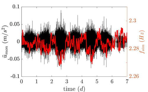
In Figure 15, the black line shows a sample time-history of the bridge acceleration at the sensor location, ${\ddot{u}}_{\mathit{mon}},$ for one week. As observed, the daily amplitude increases in the morning and decreases at night, and the response on Sunday (7th day) is significantly smaller compared to the other days. To identify the resonance frequency, the acceleration time-history resulting from response history analysis can be evaluated in the same way as the experimentally obtained data, i.e. the estimation of PSDs and subsequent peak-picking. However, since the signal comprises only one modal contribution, in the present study the so-called instantaneous frequency can be directly determined. Typically, the instantaneous frequency is calculated using the derivative of the phase angle of the Hilbert transform of the considered signal (Mathworks Inc, 2018). A more robust method for determining this quantity is to calculate the first conditional spectral moment of the time-frequency distribution of the signal referred to as spectrogram P(t, f), according to (Mathworks Inc, 2018)(9) $$f_{\mathit{sim}}(t)=\frac{{\int }_0^{\infty }f P(t,f)df}{{\int }_0^{\infty }P(t,f)df}$$(9)

Figure 15. Accelerations at monitor node ${\ddot{u}}_{\mathit{mon}}$ and instantaneous frequency f_sim from time-history analysis of one week truck traffic.

The spectrogram P(t, f) is based on a short-time Fourier transform (STFT). Due to the averaging character of the STFT, the instantaneous frequencies obtained by Equation 9(9) $$f_{\mathit{sim}}(t)=\frac{{\int }_0^{\infty }f P(t,f)df}{{\int }_0^{\infty }P(t,f)df}$$(9) are smoother than those computed by the Hilbert transform, but at the expense of the lower time resolution. The red line in Figure 15 represents the instantaneous frequency determined from the acceleration signal according to Equation 9(9) $$f_{\mathit{sim}}(t)=\frac{{\int }_0^{\infty }f P(t,f)df}{{\int }_0^{\infty }P(t,f)df}$$(9) . At first glance it can be seen that for periods with higher acceleration amplitudes the instantaneous frequency is smaller than the reference value $f_{\mathit{ref}}=2.29 Hz.$

6. Frequency shift due to mass loading

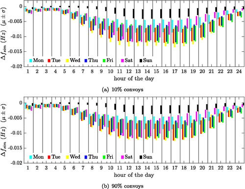
In this section, results obtained by numerical analyses employing 100 realizations of stochastically generated truck traffic of one week duration each, i.e. a total observation time of 100 weeks, are presented. Based on the results of the stochastic simulations, in the following the influence of traffic on the resonance frequency of interest is comprehensively assessed. In particular, four different simulation setups are considered: The frequency is determined both by modal analysis and by response history analysis with subsequent instantaneous frequency identification, and each method of analysis is conducted both with 10% of the trucks driving in convoys (parameter C = 0.1) and with 90% of the trucks driving in convoys (parameter C = 0.9). In each of these simulation setups, the response and subsequently the frequency of the system subjected to 100 truck traffic time histories is computed and statistically evaluated by taking the mean and standard deviation for each point in time. The averaging of these quantities in time frames in the same way as the PSD of the recorded data was estimated (i.e. four hour time segments with one hour update rate, see Section 3) results in time histories of the calculated mean resonance frequency f_sim and its standard deviation. Subtracting f_sim from the reference frequency $f_{\mathit{ref}}=2.29 Hz$ yields the frequency shift due to mass load, denoted as $\Delta f_{\mathit{sim}}.$

As the result of the calculations with modal analysis, Figure 16 shows the mean frequency shift ± standard deviation for each weekday as a function of the daytime based on an observation time of 100 weeks. The frequency shift for each weekday is illustrated by a different color. It is seen that the resonance frequency reductions are proportional to the daily variations in traffic, as shown in Figure 9(a). During the nights and on Sunday, the frequency shifts are less than $0.005 Hz,$ while during the weekdays the mean frequency shifts are about $0.01 Hz.$ Another observation is that the results based on 10% of the trucks in convoys (Figure 16(a)) and 90% of the trucks in convoys (Figure 16(b)) show only small differences. The fact that the convoy occurrence has almost no influence on the derived frequency shifts can be explained by the long averaging periods of $4 h.$ Although there are differences in the instantaneous frequency shifts between the two simulations, these differences are averaged out when calculating the mean frequency shift in this time frame. The quantitative extent of the frequency shift can be verified by a simple calculation. During one week about 30,000 trucks cross the bridge with an average dwell time of $27 s$ on the bridge. This corresponds to fictitious $30,000/(24·7)·27/3600\approx 1.5$ trucks permanently on the bridge. With an average truck mass of $30 t,$ the average mass loading is $\Delta m=45 t.$ The frequency shift due to $\Delta m$ approximated by(10) $$\Delta f=\frac{1}{2\pi }\sqrt{\frac{k^{\ast }}{m^{\ast }+\Delta m{\overline{\psi }}^2}}-f_{\mathit{ref}}$$(10) yields $\Delta f=-0.006 Hz$ when $m^{\ast }=1 kg,k^{\ast }=208 N/m$ obtained from the FE model of the bridge, and the squared mean mode shape amplitude along the bridge ${\overline{\psi }}^2=2.25·{10}^{-7}.$ This frequency shift approximates the outcome shown in Figure 16.

Figure 16. Change of resonance frequency with respect to reference value $f_{\mathit{ref}}=2.29 Hz$ (mean value μ, standard deviation σ) for two percentages of convoys, from modal analyses. 100 weeks observation time.

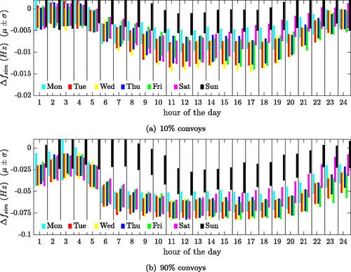
The frequency shift obtained from response history analyses are depicted in Figure 17. In contrast to the frequency shifts from modal analyses, a significant influence of the percentage of convoy occurrence is visible (note the differing ordinate scales in Figure 17(a) and (b)). While the frequency shifts obtained with 10% convoys are within the range of the results shown before (compare Figure 17(a) with Figure 16), the frequency shifts predicted from response history analyses are about seven times larger with 90% convoys than those obtained by modal analysis. Another observation is that the scatter range for the frequency shifts is significantly higher for the results from response history analysis. An explanation of this response behavior is given in the subsequent section.

Figure 17. Change of resonance frequency with respect to reference value $f_{\mathit{ref}}=2.29 Hz$ (mean value μ, standard deviation σ) for (a) 10% and (b) 90% of all trucks in convoys, from response history analyses. 100 weeks observation time.

7. Compensation of the variable mass loading effect

As discussed in the introduction, a resonance frequency that serves as performance indicator should be ‘cleaned’ of the mass loading effect. For this purpose, after determining the frequency shift for each hour of the week, a compensation value for the identified resonance frequency $f_{id}(t)$ (as shown in Figure 7) is calculated for any time instant t. For mean compensation, the mean values of $\Delta f_{\mathit{sim}}$ presented in Figures 16 and 17 are subtracted from $f_{id}(t).$ This yields the time-histories of the mass-compensated resonance frequency denoted as $f_{\mathit{comp}}(t).$ The standard deviation of $f_{\mathit{comp}}(t)$ to the corresponding standard deviation of the uncompensated frequency time-histories $f_{id}(t)$ delivers the relative change of this quantity.

For the frequency shifts based on the four different simulation setups (modal analyses/response history analyses, 10%/90% convoys), these relative changes are given in Table 4. A negative relative change represents a reduction in the time dispersion of the identified resonance frequency and is therefore a favorable result. Both the compensations that take into account the results of modal analyses and those of response history analyses with 10% convoys lead to similar outcomes. From the first three lines of the Table 4 it can be concluded that compensation of the mass loading effect does not reduce the scattering of the identified resonance frequencies in winter. This confirms the assumption that in winter climatic effects (for instance, due to freeze-thaw cycles) dominate the disturbance of the identified resonance frequency. However, compensation of this effect is out of the scope of this paper. In spring (March/April period) the compensation of the mass loading effect leads to an average reduction of the standard deviation of 4%, whereas in summer (July/August period) the average reduction is 9%. This again confirms that the mass loading effects are most relevant when temperature does not fall below freezing.

Table 4. Relative change in % of standard deviation of the identified resonance frequency over 50 days due to mass compensation (compare with Figure 7).

Period		Modal analyses		Response history analyses
		10%	90% convoys	10%	90% convoys	90%, scale 1/7
	2006/07	+1.5	+1.1	+1.8	+87.4	+2.2
Dec/Jan	2008/09	+0.3	+0.2	+0.5	+24.9	+0.5
	2010/11	+0.1	+0.0	+0.1	+28.8	+0.2
	2008	−5.0	−4.8	−4.6	+44.1	−4.1
Mar/Apr	2010	−3.5	−3.7	−3.3	+60.2	−2.9
	2011	−3.2	−3.0	−3.1	+19.1	−2.8
	2009	−8.3	−8.1	−8.0	+131.3	−5.5
Jul/Aug	2010	−8.7	−8.4	−8.7	+80.8	−8.0
	2011	−11.2	−10.7	−11.8	+87.9	−9.5

Table 4 further shows that the results of response history analyses with 90% convoys overestimates the mass loading effect, which leads to significant increases in the standard deviation of the resonance frequency time-histories. If the mean frequency shifts from Figure 17(b) are scaled by a factor 1/7, the results obtained from the compensation are consistent with the results obtained with 10% convoys, as can be seen in the last column of Table 4. Note that 1/7 corresponds approximately to the scale factor that refers to Figure 17(a) and 17(b). In an effort to further reduce the standard deviation, various scale factors were tested, but no significant improvement was found.

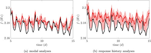
In a final investigation the effect of the standard deviation on the frequency shift presented in Figures 16 and 17 is examined. In Figure 18(a), the black graph is the identified resonance frequency over a period of 10 days in the period July/August 2011. During this period, no drastic temperature changes occurred, except for typical diurnal variations, resulting in a relatively regular resonance frequency time-history. Mean mass-compensated time-histories using frequency shifts from modal analysis and response history analysis, both with 10% convoys, are shown in red. Corresponding 95% confidence intervals (approximated by two times the standard deviations) are represented by the shaded areas. From the mean compensation curves, a significant reduction of the diurnal variations is observed. The remaining fluctuation of the resonance frequency is due to the diurnal temperature variations. While the results from the modal analyses (18(a)) show relatively narrow-banded confidence intervals, the uncertainty of the outcomes based on response history analyses (18(b)) is relatively large, since the size of the confidence interval is in the order of magnitude of the diurnal resonance frequency variation before compensation.

Figure 18. Identified resonance frequency time-history for 10 days in July 2011 (black), mass-compensated time-histories (mean values in red including 95% confidence interval).

Based on these results it can be concluded that the presented compensation approach due to time-history simulations yields relatively uncertain results. One possible cause might be the computation of the instantaneous frequency by means of Equation 9(9) $$f_{\mathit{sim}}(t)=\frac{{\int }_0^{\infty }f P(t,f)df}{{\int }_0^{\infty }P(t,f)df}$$(9) . Longer time windows for the computation of the underlying STFT would reduce the temporal scatter, but at the expense of a reduced temporal resolution, as already discussed.

8. Conclusions

In this contribution, the accelerations due to ambient loading of a freeway bridge located in the Austrian Alps from a long-term monitoring campaign were used to identify the temporal development of a resonance frequency of the bridge, which may serve as a performance indicator of the bridge. Since no structural changes or damage to the bridge were reported during the period considered, the temporal scatter of this frequency can be attributed to disturbance effects. An obvious source of disturbance is the temperature. However, in the present study the focus was put on the variable mass loading effect.

To this end, statistical data of traffic over the bridge was evaluated, and it was shown that the heavy goods traffic is highly instationary. Stochastic simulations with an FE model of the bridge were conducted to quantify numerically the effect of the time-varying truck traffic on a more global level on the considered dynamic bridge parameter. Although response history analysis represents more accurately the effect of a driving truck on the bridge, from the point of view of engineering practice, the results of this study lead to the conclusion that modal analysis seems to provide more robust and thus more reliable prediction of the frequency variation. The maximum predicted relative change of the resonance frequency due to the mass loading effect is about 0.5% (a frequency shift of $0.01 Hz$ for frequency $2.2 Hz$), and thus smaller, than the disturbance due to climatic effects. Nonetheless, in the case of performance indicators for structural damages to bridges, such as resonance frequency, the mass loading effect needs to be compensated for in order to avoid misinterpretation of the observation data. This finding can also be transferred to other freeway bridges with similar structural design, geometry and traffic volume.

The mass loading effect could also be used for other purposes: For instance, overloaded trucks can be identified in real time or the traffic volume can be inferred continuously on an entire road route. Basis for such exploitation is that the interrelationships of the mass loading effect on bridges are understood in their entirety, to which the present work aims to contribute.

Disclosure statement

No potential conflict of interest was reported by the authors.

Additional information

Funding

This work was part of the research project Street Life (project number 849045) partially funded by the Austrian Research Promotion Agency (FFG).

References

- ASFINAG. (2019). ASFINAG traffic count (in German). Retrieved from https://www.asfinag.at/verkehr/verkehrszaehlung/
- Brandt, A. (2011). Noise and vibration analysis: Signal analysis and experimental procedures. Chichester, UK: John Wiley & Sons Ltd.
- Brenner Autobahn AG. (1972). The brenner motorway (in German). Innsbruck, Austria: Verlag Tiroler Nachrichten.
- Brincker, R., & Ventura, C. (2015). Introduction to operational modal analysis. Chichester, UK: John Wiley & Sons Ltd.
- Cantero, D., Hester, D., & Brownjohn, J. (2017). Evolution of bridge frequencies and modes of vibration during truck passage. Engineering Structures, 152, 452–464. doi:https://doi.org/10.1016/j.engstruct.2017.09.039
- Chopra, A. K. (2017). Dynamics of structures (5th ed.). New York City, USA: Pearson Education.
- Clough, R. W., & Penzien, J. (2003). Dynamics of structures (3rd ed.). Berkeley, USA: Computers & Structures, Inc.
- Cross, E., Koo, K., Brownjohn, J., & Worden, K. (2013). Long-term monitoring and data analysis of the Tamar Bridge. Mechanical Systems and Signal Processing, 35(1-2), 16–34. doi:https://doi.org/10.1016/j.ymssp.2012.08.026
- Delgadillo, R. M., & Casas, J. R. (2020). Non-modal vibration-based methods for bridge damage detection. Structure and Infrastructure Engineering, 16(4), 676–697. doi:https://doi.org/10.1080/15732479.2019.1650080
- Frýba, L. (1996). Dynamics of railway bridges. London, UK: Thomas Telford.
- González, A., Rattigan, P., OBrien, E. J., & Caprani, C. (2008). Determination of bridge lifetime dynamic amplification factor using finite element analysis of critical loading scenarios. Engineering Structures, 30(9), 2330–2337. doi:https://doi.org/10.1016/j.engstruct.2008.01.017
- Ivanković, A. M., Skokandić, D., Žnidarič, A., & Kreslin, M. (2019). Bridge performance indicators based on traffic load monitoring. Structure and Infrastructure Engineering, 15(7), 899–911. doi:https://doi.org/10.1080/15732479.2017.1415941
- Kim, C., Jung, D., Kim, N., & Yoon, J. (1999). Effect of vehicle mass on the measured dynamic characteristics of bridges from traffic-induced vibration test. In Proceedings of IMAC XIX, pp. 1106–1110. Kissimmee, Florida 2001.
- Martin-Sanz, H., Tatsis, K., Dertimanis, V. K., Avendano-Valencia, L. D., Brühwiler, E., & Chatzi, E. (2020). Monitoring of the uhpfrc strengthened chillon viaduct under environmental and operational variability. Structure and Infrastructure Engineering, 16(1), 138–168. doi:https://doi.org/10.1080/15732479.2019.1650079
- Mathworks Inc. (2018). Signal Processing Toolbox user’s guide. Natick, USA: Mathworks Inc.
- Moser, P., & Moaveni, B. (2011). Environmental effects on the identified natural frequencies of the dowling hall footbridge. Mechanical Systems and Signal Processing, 25(7), 2336–2357. doi:https://doi.org/10.1016/j.ymssp.2011.03.005
- Nuttall, A., & Carter, C. (1982). Spectral estimation using combined time and lag weighting. Proceedings of the IEEE, 70(9), 1115–1125. doi:https://doi.org/10.1109/PROC.1982.12435
- Pandey, A., Biswas, M., & Samman, M. M. (1995). Damage detection from changes in curvature mode shapes. Journal of Sound and Vibration, 184(2), 311–328. doi:https://doi.org/10.1006/jsvi.1995.0319
- Peeters, B., & Roeck, G. D. (2001). One-year monitoring of the z24-bridge: Environmental effects versus damage events. Earthquake Engineering & Structural Dynamics, 30(2), 149–171. doi:https://doi.org/10.1002/1096-9845(200102)30:2<149::AID-EQE1>3.0.CO;2-Z
- Rainieri, C., & Fabbrocino, G. (2014). Operational modal analysis of civil engineering structures. New York, USA: Springer.
- Roeck, G. D., Maeck, J., Michielson, T., & Seynaeve, E. (2002). Traffic-induced shifts in modal properties. Proceedings of SPIE, 4753, 630–636.
- Sheibani, M., Hadjian-Shahri, A., & Ghorbani-Tanha, A. (2017). Mass scaling of mode shapes based on the effect of traffic on bridges: A numerical study. In Dynamics of Civil Structures, Volume 2: Proceedings of the 35th IMAC, pp. 95–106. Garden Grove, USA.
- Simeon, B., Grupp, F., Führer, C., & Rentrop, P. (1994). A nonlinear truck model and its treatment as multibody system. Journal of Computational and Applied Mathematics, 50(1-3), 523–532. doi:https://doi.org/10.1016/0377-0427(94)90325-5
- Sohn, H. (2007). Effects of environmental and operational variability on structural health monitoring. Philosophical Transactions of the Royal Society A: Mathematical, Physical and Engineering Sciences, 365(1851), 539–560. doi:https://doi.org/10.1098/rsta.2006.1935
- Sohn, H., Farrar, C. R., Hemez, F. M., Shunk, D. D., Stinemates, D. W., Nadler, B. R., & Czarnecki, J. J. (2004). A review of structural health monitoring literature: 1996–2001 (Los Alamos National Laboratory Report LA-13976-MS). Los Alamos, USA.
- Tributsch, A., & Adam, C. (2018). An enhanced energy vibration-based approach for damage detection and localization. Structural Control and Health Monitoring, 25(1), e2047. doi:https://doi.org/10.1002/stc.2047
- Veit-Egerer, R. (2014). Development of a novel, monitoring-based dynamic weighing system to describe realistically the load collective of heavy traffic and analyis of its consequence on the resulting load models on steel bridges, exemplified for the europa bridge (in German) (PhD thesis). Vienna, Austria: Technical University of Vienna.
- Veit-Egerer, R., Widmann, M., & Wenzel, H. (2008). Hot spot – Advanced weakness determination & assessment of bridges (Technical Report of FFG project 811355/3381 - GLE/BLC). VCE ZT GmbH, Vienna, Austria.
- Welch, P. D. (1967). The use of fast Fourier transform for the estimation of power spectra. A method based on time averaging over short, modified periodograms. IEEE Transactions on Audio and Electroacoustics, 15(2), 70–73. doi:https://doi.org/10.1109/TAU.1967.1161901
- Wenzel, H., & Veit-Egerer, R. (2011). Measurement-based traffic loading assessment of steel bridges – A basis for performance prediction. Structure and Infrastructure Engineering, 7(4), 261–271. doi:https://doi.org/10.1080/15732470802586428
- Westgate, R., Koo, K., & Brownjohn, J. (2015). Effect of vehicular loading on suspension bridge dynamic properties. Structure and Infrastructure Engineering, 11(2), 129–144. doi:https://doi.org/10.1080/15732479.2013.850731
- Wolf, J. P. (1994). Foundation vibration analysis using simple physical models. Upper Saddle River, USA: PTR Prentice Hall.
- Worden, K., & Cross, E. (2018). On switching response surface models, with applications to the structural health monitoring of bridges. Mechanical Systems and Signal Processing, 98, 139–156. doi:https://doi.org/10.1016/j.ymssp.2017.04.022
- Yang, Y., Lin, C., & Yau, J. (2004). Extracting bridge frequencies from the dynamic response of a passing vehicle. Journal of Sound and Vibration, 272(3-5), 471–493. doi:https://doi.org/10.1016/S0022-460X(03)00378-X
- Zhang, Q. W., Fan, L. C., & Yuan, W. C. (2002). Traffic-induced variability in dynamic properties of cable-stayed bridge. Earthquake Engineering & Structural Dynamics, 31(11), 2015–2021. doi:https://doi.org/10.1002/eqe.204