Re-deployable sensors for modal estimates of bridges and detection of damage-induced changes in boundary conditions

Abstract

Mode shapes are sensitive to the structural condition of bridges but a reasonable estimate of such changes require several accelerometers, which can be resource intensive. This paper obviates this problem through a novel structure health monitoring (SHM) approach for estimating modal parameters of bridges, including damage-induced changes of boundary conditions by using progressively re-deploying sensors along a monitored bridge. This concept of re-deployable sensors and subsequent use of a series of measurements allow extracting data from different bridge segments and also to get an indication of the condition of the bridge through frequency domain decomposition. Data from different segments are combined to estimate the global mode shape of the bridge and its gradient is observed to be indicative of support stiffness change. The concept is successfully tested through a full-scale field trial on a railway bridge in the Republic of Ireland, before and after the rehabilitation of its supports. The results are expected to guide future on-site measurement of damages due to flooding, scour, and other natural hazards, along with the effectiveness of intervention actions like repair and rehabilitation, providing a clear evidence base for practical value of SHM.

Keywords:

• Bearings
• bridges
• damage detection
• mode shapes
• re-deployable sensors
• structural health monitoring

1. Introduction

Detection and monitoring of damage or repair on a bridge can be relevant in establishing investment decisions for such repair and rehabilitation by the owner (Quirk, Matos, Murphy, & Pakrashi, 2018). It can also establish the impact of such decisions for the users and other stakeholders like the taxpayer and businesses affected by the decisions (Weninger-Vycudil, Hanley, Deix, O'Connor, & Pakrashi, 2015). While data-driven decision making using Structural Health Monitoring (SHM) can be particularly relevant in ensuring that most effective decisions are taken while maximising safety and other needs in a bridge network, lack of full-scale implementation often undermines the value of SHM. Under such circumstances, clear demonstrations of full-scale applications of novel SHM implementations can lead to a paradigm shift in terms of how decisions are eventually made on individual or a stock of bridges.

A particular problem in this regard is the detection of damage, which often manifests itself through changes in boundary conditions (Aloisio, Alaggio, & Fragiacomo, 2020; Morassi & Tonon, 2008; Majumder & Manohar, 2003; Yau, Wu, & Yang, 2001) due to flooding, scour, and other natural hazards. Such changes also take place when a repair or rehabilitation in a bridge is carried out and there is a need to assess the efficacy of such repair or rehabilitation from on-site measurements. Over its lifetime, a bridge is increasingly exposed to natural hazards and the relevance of this problem is thus fundamentally linked its safety and functionality.

To address damage detection of this nature, it is important to be able to estimate the mode shapes of a bridge in field-conditions and ensure that changes in such mode shapes are detected due to damage. This is a challenge by itself since higher mode shapes are more sensitive to damage but more uncertain in their estimates while the more consistently measured lower mode shapes are less sensitive to damage. Additionally, the estimation of a mode shape requires measurements at multiple locations on the bridge, which in turn requires access to several accelerometers (Gomez, Fanning, Feng, & Lee, 2011; Kim, Ryu, Cho, & Stubbs, 2003; Shi, Law, & Zhang, 2000; Shih, Thambiratnam, & Chan, 2013). This can be resource intensive and may require the closing down of the bridge, leading to significant loss of tangible and intangible financial resource (Pakrashi, Kelly, & Ghosh, 2011). Extensive instrumentation requiring bridge closure is also related to safety of traffic and workers and can be difficult to maintain. Consequently, an effective SHM method for practical applications must be sensitive to damage, stable in terms of measurement and with minimised impact on the operations of the bridge. Minimisation of instrumentation needs would also be preferable to establish its value.

The recently concluded EU Cooperation in Science and Technology (COST) Action TU1402 established the needs for demonstrating the value of SHM in different fields of operation, with its quantification being firmly rooted in full-scale evidence bases. The action focused on the relevance on optimal sensor placement and robust metrics (Leyder, Dertimanis, Frangi, Chatzi, & Lombaert, 2018; Žnidarič, Kalin, & Kreslin, 2018) and in-service monitoring relevance (Thöns et al., 2017).

This paper addresses the practical problem of detecting damage in bridges through changes in mode shapes due to damage induced variations of boundary conditions by using re-deployable sensors along the bridge and assembling data from each-segment in a bespoke manner. Accelerometers are ubiquitous as a choice for mode shape measurement (Doebling, Farrar, & Prime, 1998; Hester & González, 2015) and they can be instrumented to the bridge or the vehicle traversing it. Strain gauges can detect damage but generally need to be significantly close to the damage location for localised damages in which bridge strain due to damage peaks sharply within a very short length close to the damage location (Carneiro & Inman, 2002; Pakrashi, Harkin, Kelly, Farrell, & Nanukuttan, 2013). Strain gauges can thus require extensive instrumentation and can be disruptive to traffic.

The decentralised approach, used in this paper, provides the advantage of obtaining data from relatively denser monitoring points than what we would have achieved with static sensors. In the absence of re-deployable strain gauges, this method of using accelerometers provides a particular advantage, as has been demonstrated in the paper. The changes in boundary conditions can be due to varied causes including scour from flooding and gradual degradation of bearings due to daily wear. Overall, such damage or changes are typically linked to changes in rotational stiffness at the supports (Kliewer & Glisic, 2017), for which an array of strain sensors is often unfeasible due to practical challenges on site despite numerical or small-scale experimental feasibility studies (Kliewer & Glisic, 2017). In fact, repair or rehabilitation of such damage will also demonstrate a change in rotational stiffness as compared to the damage state or the reference state.

Deviation of mode shapes due to damage has been characterised through changes in curvature (Kliewer & Glisic, 2017), change in modal energy (Shi et al., 2000) and similar markers. However, the process of measuring the curvature involves the differentiation of bridge accelerations which is prone to errors. Densely spaced strain gauges can avoid this problem, but it comes with the aforementioned challenges of bridge closedown and sensor maintenance problems along with traffic and worker safety.

An alternative approach to this is the bourgeoning idea in the literature around using the responses of bridge-vehicle interaction (Pakrashi, O'Connor, & Basu, 2010) and then obtaining modal (natural frequency, damping, mode shape) and damage information indirectly. This approach reduces instrumentation but introduces variability from road surface roughness (Jaksic, O’ Connor, & Pakrashi, 2014). Additionally, there is a paucity in literature in full-scale implementation of estimating relevant features of interest of a bridge by utilising the interaction with a moving vehicle. For example, Zhang, Wang, and Xiang (2012) estimate bridge mode shape squares from the vehicle accelerations and take them as a damage index while Yang, Li, and Chang (2014) extend this research by constructing the bridge mode shapes theoretically using responses from a passing vehicle.

Recently, a method of Short Time Frequency Domain Decomposition (STFDD) has been proposed which estimates bridge mode shapes using a multi-stage series of acceleration measurements (Malekjafarian & OBrien, 2014, 2017). The multi-stage process estimates segments of mode shape using the Frequency Domain Decomposition (FDD) concept (Brincker, Zhang, & Andersen, 2001) and connects them using common points between neighbouring segments (Sim, Spencer, Zhang, & Xie, 2010). A main criticism of the STFDD drive-by method is that it is critically influenced by vehicle velocity, thereby making it difficult to detect damage unless it is travelling at an unrealistically slow speed. Direct decentralised and multi-setup approaches for modal analysis have been proposed for modal estimation techniques, that use independent groups of measurements with overlapping nodes to capture local spatial information in stitch-able segments (Sim et al., 2010), or reference-based multi-setup stochastic subspace identification algorithms (Döhler, Lam, & Mevel, 2013).

Sim et al. (2010) analysed different sensors topologies to study the effect of changing overlapping nodes on the accuracy of the estimated global mode shapes, and Döhler et al. (2013) computed statistical uncertainties and covariance mode shapes derived using multi-setup subspace system identification algorithm and applied the approach on bridge ambient vibration data. Although, these direct approaches provide successful results using free or ambient vibrations of the structure, the effect of forced vibrations caused by moving vehicles, still poses a challenge for the decentralised modal estimation techniques. The forced vibrations provide higher amplitude of bridge dynamic responses due to heavy traversing loads as compared to the free or ambient vibrations, hence, resulting cleaner signals and sharper frequency peaks. Therefore, the forced vibrations may facilitate the mode shape estimation and damage detection technique proposed in this paper.

This paper addresses several of the challenges described in this section with a focus around practical implementation. A bespoke method is proposed here where a small number of sensors are moved along the bridge and are re-deployed for various segments (by changing the location of the sensors on the bridge with time and independently of traffic movement) to obtain the modal parameters and the variations due to damage in the form of changes in rotational stiffness of the boundary condition of the bridge. This approach does not need indirect methods of analyses, which is typical for drive-by measurements using instrumented vehicles for which vehicle conditions are required to be known precisely and uncertainties are introduced in real life from lack of control over the vehicular characteristics and their movement. The proposed approach with re-deployable sensors allows a high-density array of measurement points to be monitored without using a large number of sensors.

In this work, a novel approach of using bridge forced vibrations due to traversing vehicles is proposed to offer a more repeatable testing condition and cleaner signals than free vibrations, which have been used in the past, but exhibit significantly lower response amplitudes. A sequence of movements ensures that accelerations are recorded over the full span of the bridge. Subsequently, the FDD technique (Brincker et al., 2001) is applied to the bridge accelerations to calculate segments of mode shape, which are subsequently stitched together at common locations to create a global mode shape. Change in the global mode shape with different bridge bearing condition changes is studied for damage detection. To initially establish the feasibility of the idea numerically, a simplified vehicle model is simulated traversing a beam with rotational springs at the supports (Cantero, O'Brien, & González, 2010; González, 2010; Yang & Lin, 2005) to represent bridge bearing stiffness (Kliewer & Glisic, 2017). A typical class ‘A’ road profile is randomly generated (Tyan, Hong, Tu, & Jeng, 2009) for a road surface and the bridge acceleration responses are analysed (Bathe & Wilson, 1976) to determine the mode shape segments at relevant locations, along with the changes of the mode shapes due to damage.

The first mode shapes have been used to numerically demonstrate the concept of re-deployable sensors and the first global mode shape, along with its gradient, is observed to be an effective way of detecting damage. The idea is then established in a comprehensive fashion by demonstrating its implementation through a full-scale test on a railway bridge in the Republic of Ireland and considering before and after scenarios of damaged and rehabilitated conditions. The results from these field tests demonstrate and quantify the effectiveness of the proposed concept in damage detection and provides key evidence in establishing its value for implementation at a wider scale by the owners of bridge infrastructure. This work also has the potential to be applied to the renewable energy sector (Buckley, Watson, Cahill, Jaksic, & Pakrashi, 2018) where changes in boundary condition from soil-structure interaction can be a significant problem in terms of lifetime performance and design of control systems.

2. Numerical estimation of mode shapes within a re-deployable sensor framework

2.1. The bridge-vehicle interaction model

A bridge is idealised as a finite element (FE) model (Figure 1) of a simply supported beam (González, 2010) spanning 20 metres. It consists of 20 discrete beam elements, each with 4 degrees of freedom (DOF) (2 per node—vertical translation and in-plane rotation) (González, 2010). The horizontal translation is not included in the analysis given that axial deformations in the beam element can be neglected due to a lack of loading in that direction. To represent realistic bridge support conditions, a spring is added at each support with rotational stiffness (K_rot). This spring is added in a way that provides additional restraint to the rotational DOF at both bridge ends without adding extra DOFs in the model. The value of K_rot in reality lies somewhere between 0 (free to rotate) and infinity (fully fixed). The mechanical properties of the bridge with simply supported boundary conditions and the first three natural frequencies are shown in Table 1.

Figure 1. An idealized bridge model with support degradation traversed by a quarter-car vehicle.

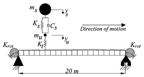
Table 1. Properties of the bridge model.

Bridge Property	Notation	Value
Total no. of degrees of freedom	n	42
Young's Modulus	E	35 × 10^9 N/m^2
Breadth	w	5 m
Depth	d	1 m
2^nd moment of area	J	0.417 m^4
Mass per unit length	µ	12500 kg/m
Damping	ξ	3%
1^st natural frequency	f1	4.24 Hz
2^nd natural frequency	f2	16.97 Hz
3^rd natural frequency	f3	38.18 Hz

A sampling frequency (f_s) of 500 Hz is used when simulating bridge accelerations, which vary with time based on the position of the passing vehicle. A location matrix, N_b (n_a x n_s), is calculated for each axle location on the bridge where n_s is the total number of time steps and n_a is the number of vehicle axles. An approach length of 100 metres is added to ensure equilibrium before the vehicle arrives on the bridge (McGetrick, Kim, González, & Brien, 2015). A class ‘A’ road surface profile is generated according to the ISO standard (ISO, 1995) with a geometric spatial mean of 16 × 10⁻⁶ m³/cycle and added to the model (Keenahan, OBrien, McGetrick, & Gonzalez, 2014). Bridge dynamic response to time-varying forces is calculated at each time step (McGetrick, González, & OBrien, 2009) using the system of equations as: (1) $${\mathrm{M}}_{\mathrm{b}}{\ddot{\mathrm{y}}}_{\mathrm{b}}+{\mathrm{C}}_{\mathrm{b}}{\dot{\mathrm{y}}}_{\mathrm{b}}+{\text{ K}}_{\mathrm{b}}{\mathrm{y}}_{\mathrm{b}}={\mathrm{N}}_{\mathrm{b}}{\mathrm{f}}_{\mathrm{int}}$$(1) where K_b, C_b and M_b are the (n x n) bridge stiffness, damping and mass matrices, respectively, and ${\mathrm{y}}_{\mathrm{b}},$ ${\dot{\mathrm{y}}}_{\mathrm{b}}$ and ${\ddot{\mathrm{y}}}_{\mathrm{b}}$ are the (n x n_s) vectors of bridge nodal displacements, velocities and accelerations, respectively. The term f_int is the vector of total bridge and vehicle interaction forces at each axle contact point calculated using the road profile and the bridge displacement under each vehicle axle.

The bridge is assumed to be simply supported in its healthy state and to have gained rotational stiffness at the supports due to deterioration (Kliewer & Glisic, 2017). Thus, K_rot changes from zero to a finite value as the supports become constrained, thereby resulting in changes in mode shapes. A quarter-car (Figure 1) model of vehicle, which is a simplified manifestation of a moving axle, is considered consisting of 2 DOFs corresponding to sprung mass bounce (y_s) and axle hop (y_u), respectively (McGetrick, González, & O'Brien, 2010). The mechanical properties of the quarter-car considered in this paper (Keenahan et al., 2014) are shown in Table 2. The sprung mass (m_s), and the unsprung axle mass (m_u) are connected through a linear spring with stiffness K_s and a viscous damper with damping coefficient C_s. The axle mass is connected to the road surface via another spring with stiffness K_t.

Table 2. Mechanical properties of the idealized quarter-car adapted from (Keenahan et al., 2014).

Quarter-Car Vehicle Property	Notation	Value
Unsprung mass	mu	700 kg
Tyre stiffness	Kt	1.75 × 10^6 N/m
Suspension stiffness	Ks	40 × 10^4 N/m
Suspension damping	Cs	10^4 Ns/m

The equations of motion for the vehicle model, expressed in terms of vehicle DOFs, are created by imposing equilibrium of the forces (González, 2010) acting on the masses: (2) $${\mathrm{M}}_{\mathrm{v}}{\ddot{\mathrm{y}}}_{\mathrm{v}}+{\mathrm{C}}_{\mathrm{v}}{\dot{\mathrm{y}}}_{\mathrm{v}}+{\mathrm{K}}_{\mathrm{v}}{\mathrm{y}}_{\mathrm{v}}={\mathrm{f}}_{\mathrm{v}}$$(2) where K_v, C_v and M_v are the (n_v x n_v) stiffness, damping and mass matrices of the vehicle respectively, and ${\mathrm{y}}_{\mathrm{v}},$ ${\dot{\mathrm{y}}}_{\mathrm{v}}$ and ${\ddot{\mathrm{y}}}_{\mathrm{v}}$ are the (n_v x n_s) vectors of vehicle displacements, velocities and accelerations respectively. The f_v vector represents the dynamic interaction forces applied to the vehicle by the road profile and the bridge displacements.

The bridge and the vehicle models are coupled in a global coordinate system at each axle contact point to implement the dynamic interaction (González, 2010) between them as: (3) $${\mathrm{M}}_{\mathrm{g}}\ddot{\mathrm{u}}+{\mathrm{C}}_{\mathrm{g}}\dot{\mathrm{u}}+{\mathrm{K}}_{\mathrm{g}}\mathrm{u}=\mathrm{F}$$(3) where M_g and C_g are the coupled ((n + n_v) x (n + n_v)) mass and damping matrices, respectively, K_g is the time-varying coupled stiffness matrix that depends on the axle locations and the bridge static displacements due to vehicle loading and F is the system force vector (McGetrick et al., 2009). The vectors, $\mathrm{u},$ $\dot{\mathrm{u}}$ and $\ddot{\mathrm{u}}$ ((n + n_v) x n_s) contain the modal displacements, velocities and accelerations of the system, respectively. The equations of the coupled system are solved using the Wilson-Theta integration scheme (Bathe & Wilson, 1976), with θ = 1.420815 for unconditional stability in the integration process.

2.2. Re-deployable sensors for bridge mode shapes estimation

The modal properties of the bridge are estimated using a sequence of measurements from a small set of accelerometers that are moved from one end of the bridge to the other. In this study, only two accelerometers (Ac1 & Ac2 in Figure 2) are considered at any given instant of time. These accelerometers are re-deployed to different bridge nodes at different time instants. This re-deployment of accelerometers is independent of the location and speed of the moving vehicles. The bridge acceleration responses at each node undergo a Frequency Domain Decomposition (FDD) and an estimated mode shape for each measured segment between two measured nodes is created for a desired frequency from the spectral densities of the accelerations in the frequency domain (Brincker et al., 2001). Numerically, the bridge accelerations due to the quarter-car passage were calculated using the equations of the coupled system in the previous section.

Figure 2. A Visual Schematic of the proposed accelerometer redeployment concept.

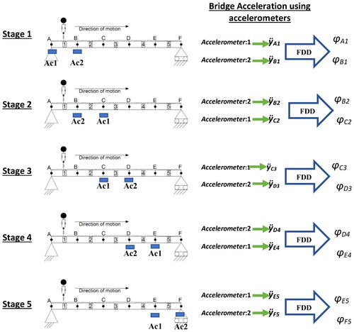
Figure 2 illustrates the proposed concept applied in five stages. In each stage, FDD gives a vector of mode shape amplitudes [φ_li, φ_ri] for a segment of mode shape, where l and r are the left and the right ends of the segments, respectively and i is the stage number. It should be noted that to implement the concept of re-deployable sensors, neighbouring segments must be contiguous to allow consistent rescaling and subsequent combination to create a global mode shape. This is achieved by allowing one accelerometer to stay fixed in a segment while the other moves to the next.

The use of FDD enables the estimation of segments of bridge mode shape without prior knowledge of vehicle parameters, which is advantageous over several drive-by approaches. Mode shape amplitudes are obtained by decomposing the power spectral density matrix (Ĝ(jω_i)) through Singular Value Decomposition (SVD) for each frequency i of the acceleration response (Brincker et al., 2001; Hoskere, Park, Yoon, & Spencer, 2019; Malekjafarian & OBrien, 2014) as: (4) $$\widehat{G}\left(j{\omega }_i\right)=\mathrm{ }{U}_i{S}_i{U}_i^H$$(4) where U_i is the unitary matrix of singular vectors, S_i is a diagonal matrix containing singular values and H denotes the complex conjugate of the matrix. Mode shape amplitudes are calculated as the singular vectors corresponding to a selected frequency. Details of the FDD method are provided in (Brincker et al., 2001).

To obtain a global mode shape, the segments are stitched together using the decentralised modal analysis procedure (Sim et al., 2010). This combines the mode shape amplitudes at the common locations by rescaling them. The rescaling factor, R_s, is calculated as the ratio between the mode shape amplitude at the s^th stage common location to the one at the (s + 1)^th stage. The global mode shape (${\mathrm{\varnothing }}_{\psi }^i$) for a frequency i, using the r number of segments [ψ_1, ψ_{2, …} ψ_r], is then given by: (5) $${\mathrm{\varnothing }}_{\psi }^i={\cup }_{s=1}^r{R}_s{\psi }_s$$(5)

2.3. Numerical validation of the proposed concept

Bridge accelerations are simulated using the vehicle-bridge interaction model presented (González, 2010) and segments of mode shapes are calculated using the FDD algorithm (Malekjafarian & OBrien, 2014). The mode shape segments are stitched together using Equation (5)(5) $${\mathrm{\varnothing }}_{\psi }^i={\cup }_{s=1}^r{R}_s{\psi }_s$$(5) to generate the global mode shape. In this work, the first three mode shapes of the bridge model, shown in Figure 1, are estimated using the proposed concept.

The span is divided into 5 equal segments, each having a length of 4 m, with nodes at 0, L/5, 2 L/5, 3 L/5, 4 L/5 and L respectively (Figure 2). The healthy bridge condition corresponds to a perfectly pinned support. For each stage, the body mass and vehicle velocity of the quarter-car are chosen randomly, based on a Monte Carlo simulation (Figueiredo, Radu, Worden, & Farrar, 2014), drawing from Normal distributions with means and standard deviations of typical two-axle traffic data. White noise (OBrien & Keenahan, 2015) with a mean of 0 and 5% of the forced signal standard deviation which depends on the moving vehicles’ mass and speed parameters, is added to the acceleration responses to allow for possible measurement inaccuracy.

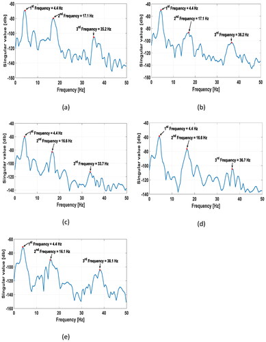
For each stage, the bridge accelerations are calculated at the left and right ends of the segment of interest starting from the arrival of the quarter-car model on the bridge until 2 seconds after it exits regardless the velocity of the vehicle. Consequently, the signal consists of a mix of forced and free vibration responses. The SVD diagrams from the 5 stages (Figure 3) indicate that at each stage the dominant peaks are present at or near the bridge natural frequencies. The difference in the frequencies between the true values (from Table 1) and those found from the SVD diagrams, can be explained by the effect of the moving load (Cantero, Ülker-Kaustell, & Karoumi, 2016).

Figure 3. SVD Diagrams for (a) stage 1; (b) stage 2; (c) stage 3; (d) stage 4; (e) stage 5.

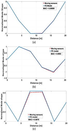
The singular vectors for the first three bridge frequencies are obtained from the labelled peaks in the SVD diagrams (see Figure 3) and define the local mode shape for each segment. By applying the rescaling process, the first three global mode shapes are calculated. These have been normalised and compared with the exact mode shapes obtained from the FE model in Figure 4. The MAC values (Malekjafarian & OBrien, 2014) for the first three mode shapes, compared with the theoretical eigen-value mode shapes, are all greater than 0.9975, suggesting a good accuracy, with lower values for higher modes as expected.

Figure 4. Bridge mode shapes measured using the concept of moving sensors: (a) 1st mode shape; (b) 2nd mode shape; (c) 3rd mode shape; MAC = Modal Assurance Criterion.

2.4. Influence of rotational stiffness on mode shape

Damage in the form of bearing stiffness is chosen to be investigated in this paper as an illustrative case. Bearing damage introduces constraints at the boundaries of the bridge in the form of rotational stiffness and thus changes modal properties. The degree of damage is related to the magnitude of rotational stiffness. The first translational mode shape (in vertical direction) is measured most accurately and is relatively easy to obtain in site. Additionally, the static deflected shape is often a reasonable approximation of the first translational mode shape. The gradient of the first mode shape is used an indicator of damage.

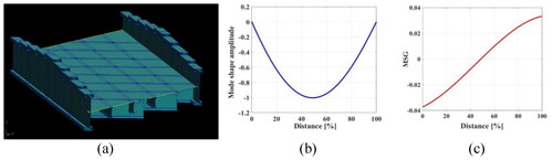
The support bearing damage is simulated numerically by increasing the K_rot value, starting from 0 Nm (the healthy condition) and increasing to a value of 10¹² Nm, at which point, the supports start behaving almost like a beam with two fully fixed (mode shape gradient at support (support gradient) = 93% of fully fixed) ends. The body mass and the velocity of the quarter-car model are taken as 10 t and 20 m/s respectively while other properties are kept constant as in Table 2. The first natural frequencies (Table 3) and translational mode shapes (Figure 5) are calculated for different values of K_rot reflecting the degree of support stiffness. In the context of Table 3, the severity is defined based on the percentage of mode shape gradient to a fully-fixed bearing condition. The change in the natural frequency, which is typical of any damage case, is used in this paper as a secondary parameter to verify change in the bridge condition. The bridge frequency corresponding to K_rot = 10¹² Nm and K_rot = 10¹³ Nm are close, showing that the bridge supports have nearly reached fixed support condition. Figure 5 also indicates that increasing the stiffness of the supports reduces the gradient of the first mode shape at those points.

Figure 5. Numerically obtained first mode shape of an idealized bridge with different damage constraints at the boundaries.

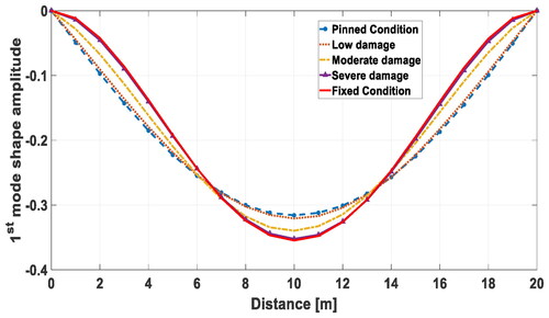
Table 3. First natural frequency of an idealized bridge for different percentages of K_rot obtained numerically.

Krot (Nm)	0	10^9	10^10	10^11	10^12	10^13
Support gradient (% of fully fixed value)	0	3	12	55	93	99
Damage Condition	Pinned	Low	Moderate	Severe	Fixed	Fixed
Bridge 1^st Frequency (Hz)	4.24	5.18	7.81	9.35	9.60	9.64
Difference in Frequency (%)	0	22	84	121	126	127

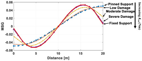
The Mode Shape Gradients (MSGs) of the first mode shape are plotted in Figure 6. The use of MSGs can be seen to amplifies the effect of changing support stiffness. The general trend is a change from a sigmoid shape for the simply supported state, towards an approximate sine wave shape for the fixed-fixed state. The increase in K_rot percentage forces the MSG at the support toward a value of zero and demonstrates reasonable sensitivity to this change. It can be seen in Figure 6 that the MSG indicator can effectively detect moderate damage of the bearing condition which corresponds to almost 12% of fully fixed mode shape gradient value. Therefore, in this paper, the MSG curve is used as one of the indicators of changes in the bridge support condition.

Figure 6. Numerically obtained First Mode shape gradient for different support stiffnesses for an idealized bridge.

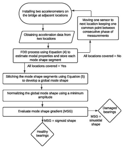
The flowchart of the proposed approach for detecting bridge bearing seizure is illustrated in Figure 7. It should be noted that in this paper, the approach is developed based on one type of bridge damage—bearing failure, instead of combination of different types of damages. For any combined case, it will be difficult to inverse-model and detect the difference only using this one scheme of re-deployable sensors, especially if they are overlapping in their effects. On the other hand, damages due to stiffness loss within the structure can be picked up by re-deployable sensors even with bearing rotational stiffness deterioration, since it will be identified in a different set of experiments. The topic of inverse detection of combined damage from various sources remains a challenging topic.

Figure 7. Flowchart of the proposed approach.

3. Experimental validation of modal parameters and damage effects using the proposed re-deployable sensor framework

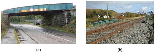
The proposed concept of using re-deployable sensors was validated next through a full-scale study. The Oranmore bridge (UBG165) (Figure 8) in Co. Galway, Republic of Ireland was selected for this purpose. UBG165 has an 18.3 m long single-span skewed steel deck and carries one operational rail track. The bridge consists of 2 primary longitudinal, 8 secondary transverse and 4 tertiary longitudinal steel beams with a thin steel plate deck. The bridge is 8.8 m wide and is skewed at an angle of 48.5^°.

Figure 8. The Oranmore Bridge: (a) North side from the South; (b) top of the bridge from the West.

There was uncertainty about the support conditions (Figure 9) and the bridge was rehabilitated on 26^th October 2019. The ends of the deck were repaired and new bearings and abutments were installed (Figure 10). Re-deployable accelerometers were used to assess the bridge before refurbishment on 15^th–16^th of October and then again after refurbishment on 12^th–13^th November. The field tests utilised bridge accelerations induced by passing trains and the first bridge mode shape was estimated before and after the replacement of support bearings.

Figure 9. Support conditions of the Oranmore bridge - before rehabilitation: (a) primary longitudinal beam; (b) tertiary beam.

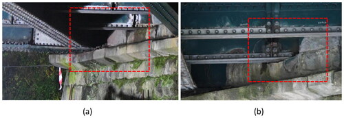
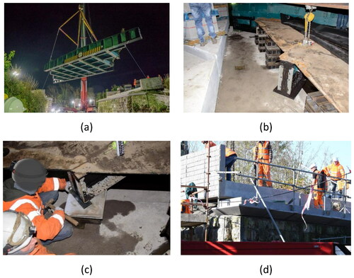
Figure 10. The rehabilitation of Oranmore bridge: (a) deck lift; (b)view on top of new precast concrete abutments and bearings; (c) bridge support bearing installation; and (d) side view of new precast concrete abutments.

3.1. Rehabilitation details

Before the rehabilitation, the Oranmore bridge was inspected by the Irish operator and identified as being affected by inadequate bridge support conditions. Figure 9 illustrates the support conditions before the rehabilitation. Two primary, two secondary and two tertiary beams were resting on stone abutments at both sides of the bridge with unknown restraints to rotational capacity of the beams. Following refurbishment, the constraints at the boundaries were released and the field-implementation aimed to see if damage resulting in non-zero support stiffness could be identified following refurbishment.

The replacement of the supports of the Oranmore bridge took place on the 26^th of October 2019. The rails were cut, and ballast removed to clear the deck, which was then lifted using a crane (Figure 10(a)) and placed on the road below. The bridge was out of operation for two days while the rehabilitation took place. The abutments were replaced with a precast concrete transition slab and elastomeric bearings fitted at the beam ends. Other minor repairs were carried out on rusted areas of the bridge.

3.2. Instrumentation details

Two triaxial wireless MEMS accelerometers (LORD MicroStrain G-Link-LXRS) were used to record the deck accelerations due to passing trains before and after the rehabilitation. Technical specifications of the accelerometers are mentioned in Table 4. In order to maintain time-synchronisation (Veluthedath Shajihan et al., 2020), a sensors’ in-built beacon-based time-synchronisation tool is used, which is facilitated by a gateway, that communicates wirelessly to all the sensors before measuring the bridge accelerations in each stage. Six measurement locations were selected on the primary beam on the North side (Figure 11). Testing was carried out in 5 stages, each involving sensors at two locations on the beam, while always keeping one location in common with the neighboring segment/stage. These correspond to A-B, B-C, C-D, D-E and E-F in Figure 11.

Figure 11. Meaurement locations on primary beam on North side: (a) elevation with dimensions (in mm) and percentage of span; (b) photograph.

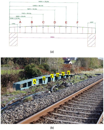
Table 4. Technical specifications of LORD G-Link/LXRS accelerometers.

Sensors’ Property	Value
Measurement range	± 10 g
Accuracy	10 mg
Resolution	12 bit
Sampling frequency	256 Hz
Sampling mode	Synchronized

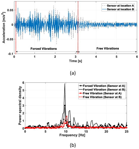
The accelerometers were attached to the beam web at each location using magnetic mounting bases and accelerations were recorded at a scanning rate of 256 Hz. Recharging of the accelerometers was carried out after each phase using a car battery and DC inverter. It has been observed that in most of the measurements, the acceleration response damps out instantly after the train leaves the bridge, making it difficult to estimate mode shapes using only free vibrations. For that reason, the modal estimation is carried out using the forced accelerations, which provided reasonable excitation in the bridge. An example of measured acceleration responses at locations A and B before rehabilitation, in time and frequency domain are shown in Figure 12(a) and 12(b), respectively. For each stage of measurement, the accelerations in response to 3 passing trains were recorded and transmitted wirelessly to a base station near the bridge. Recording was continued for two seconds of free vibrations after the passage of each train.

Figure 12. Acceleration signals (forced and free vibrations) from bridge locations C and D (before rehabilitation); (a) in time domain; and (b) in frequency domain.

3.3. Development of a numerical model of the bridge

To compare the first mode shape of the bridge for the healthy support condition with that obtained from full-scale experimentation, a Finite Element (FE) model of the bridge was created in PATRAN/NASTRAN 2018 (Figure 13(a)). Typical steel properties were assigned to all elements and pinned supports were assumed on both ends. The first mode shape is illustrated in Figure 13(b) and its gradient in Figure 13(c). These are used as damage indicator reference values in this study. For practical deployments, such a model is useful but is not a must if the unconstrained experiment is consistent and if there is confidence about the freedom at the boundaries.

Figure 13. The Oranmore bridge numerical model: (a): the FE model; (b) calculated 1st bridge mode shape; and (c) the 1st bridge mode shape gradient.

3.4. Experimental results and discussion

The first natural frequency of the bridge is calculated experimentally using a Fast Fourier Transform (FFT) from the forced and free vibration signals for each passing train (Table 5). It can be seen from Table 5 that the average frequencies have decreased after the rehabilitation for both forced and the free vibrations. This change is consistent with a release of support stiffness due to the installation of new bearings (see Table 3). The frequency change in Table 3 for the numerical study is higher due to the idealised conditions. However, in reality the deviation obtained from experimentation is, although lower than the numerical model but is reasonably high and indicates that the stiffness change is approximately 10%, indicating that a definitive change in structural condition has occurred. Although this change indicates significant bridge damage, further mode shape analysis must be carried out to detect specific bridge bearing seizure.

Table 5. First bridge natural frequency from the bridge accelerations to each passing train at UBG165.

1^st Natural Frequency
Before bridge rehabilitation					After bridge rehabilitation
Sensor locs.	Train No.	Route	Forced Freq./ Hz	Free vibration freq. /Hz	Train No.	Route	Forced Freq./ Hz	Free vibration freq. /Hz
A & B	1	Galway to Dublin	10.15	10.32	16	Galway to Dublin	9.66	9.64
	2	Limerick to Galway	9.72	10.26	17	Limerick to Galway	9.51	9.65
	3	Dublin to Galway	9.16	10.23	18	Galway to Dublin	8.98	9.65
B & C	4	Galway to Dublin	10.18	10.25	19	Dublin to Galway	7.20	7.39
	5	Dublin to Galway	10.10	10.27	20	Limerick to Galway	9.00	9.62
	6	Galway to Limerick	10.12	10.26	21	Dublin to Galway	9.29	9.62
C & D	7	Limerick to Galway	9.72	10.25	22	Galway to Limerick	9.59	9.65
	8	Dublin to Galway	10.54	10.33	23	Galway to Dublin	7.17	7.31
	9	Galway to Dublin	10.43	10.48	24	Limerick to Galway	9.84	9.66
D & E	10	Limerick to Galway	10.05	10.28	25	Dublin to Galway	7.31	7.65
	11	Dublin to Galway	10.04	10.10	26	Dublin to Galway	9.46	9.61
	12	Limerick to Galway	9.25	10.25	27	Limerick to Galway	9.37	9.65
E & F	13	Galway to Dublin	9.98	10.14	28	Galway to Dublin	9.49	9.57
	14	Galway to Limerick	9.03	10.01	29	Galway to Limerick	9.28	9.62
	15	Galway to Dublin	9.59	9.80	30	Galway to Dublin	7.24	7.38
Avg.			9.85	10.22	Avg.		8.83	9.05

The data from each stage of the field test is analysed using FDD to obtain a segment of the first mode shape. For each stage, the mode shape segment is calculated three times, once for each of the passing trains. Over five stages, with three segments of mode shape per stage, there are (3⁵=) 243 possible ways in which the segments can be combined. All 243 estimates of the mode shape are normalised and presented in Figures 14 and 15(a) for the pre- and post-rehabilitation measurements. A second statistical estimation based on a Monte Carlo approach (Figueiredo et al., 2014) is also carried out to assess the uncertainty of the estimated mode shapes. A mean and a standard deviation of modal amplitudes are used to randomly generate 500 modal amplitudes for each sensor location which are then stitched together to obtain 500 global mode shapes.

Figure 14. Normalised 1st bridge mode shape of the Oranmore bridge from 243 combinations: (a) before rehabilitation; (b) after rehabilitation.

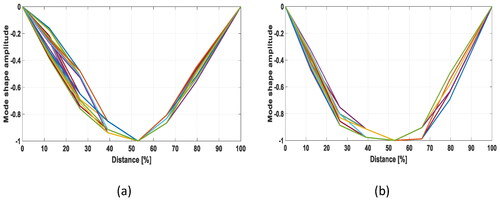
Figure 15. Mean ± one standard deviation of 1st bridge mode shape before and after the rehabilitation; (a) using 243 combinations; (b) using Monte Carlo estimation.

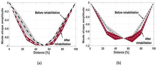
The normalised mode shapes for the pre- and post-rehabilitation measurements, using the Monte Carlo estimation, are shown in Figure 15(b). It can be seen in Figure 15(a) and (b) that there is considerable overlap in mode shape values near the peak (normalisation) point. However, this is not the case for other points and, when the whole mode shape is taken together, the differences are clear. There is a significant difference between the two mode shapes, with the post-rehabilitation mode shapes being more U-shaped towards the centre. This change is due to a lower support stiffness and is consistent with the numerical results shown in Figure 5.

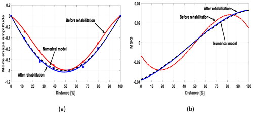
To obtain a finer resolution of the mode shape (as only five sample points were monitored in the field tests), a 4^th degree polynomial is fitted to the mean mode shape (Figure 16(a)). The post-rehabilitation fitted mode shape matches well with the numerical FE model results (shown in Figure 13(b)) and is significantly different from the pre-rehabilitation shape. The gradients of the fitted mode shapes are illustrated in Figure 16(b). Again, the post-rehabilitation result is a good match to the numerical FE model results (shown in Figure 13(c)). The pre-rehabilitation MSG shape is clearly different and is close to the shape of a sine wave than a sigmoid shape (see Figure 6). Both mode shape amplitude and MSG can be seen to be appropriately robust indicators of support condition.

Figure 16. Damage indicators before and after rehabilitation; (a) fitted 1st bridge mode shape; (b) Mode Shape Gradient (MSG).

4. Conclusions

This paper presents a novel measurement and analyses strategy for bridge structural health monitoring to assess damages due to changes in support conditions. The approach utilises a low number of re-deployable accelerometers to estimate modal parameters by combining estimated mode shapes at various segments of the bridge and subsequently compute damage indictors. The proposed method demonstrates its application on damages in bridge bearings. For both forced and free-vibration data form bridge-vehicle interaction due to random traffic, the changes in the first translational mode shape and its gradient were observed to be consistently indicative of damages related to changes in rotational constraints at the boundaries.

The proposed concept, by using the forced vibrations due to passing random vehicles, reduces field instrumentation, avoids a need of sensitivity analysis and indirect computation from instrumented drive-by vehicles and their related uncertainties allowing a bridge to remain operational. The approach can also be used to establish the efficacy of repair and rehabilitation work. The proposed approach was numerically demonstrated to be feasible. Subsequently, the concept was tested successfully on a full-scale bridge before and after a bearing change. Only two accelerometers were adequate to demonstrate the proposed concept in field conditions, by moving them progressively along one of the primary beams of the bridge with three train passages occurring between each move. The numerical study and the field study concur in their overall observation.

The key findings of this study are as follows:

1. In the numerical analysis, the re-deployable sensors concept effectively calculated the first three mode shapes with MAC values in excess of 0.9975.

2. In the numerical analysis, the first mode shape and its gradient undergo a definitive change due to bearing damage. The shape of the gradient curve in particular, is an effective indicator of support stiffness.

3. In the field analysis, the first mode shape of the bridge after rehabilitation closely resembles the numerically generated mode shape with simple supports. The mode shape and its gradient successfully indicate the change in support conditions, due to rehabilitation.

Bridge mode shapes are sensitive to changes in support condition, and the possibility of using the re-deploying sensors concept for detecting bridge bearing/abutment damage appears to have excellent potential. The approach can also be helpful for bridges that have undergone scour damage, damage due to flooding and earthquake. The work can also be relevant for monitoring the soil-structure interaction conditions of onshore and offshore wind turbines along with intervention designs like the installation of a passive controller. Bridge monitoring using this approach in a case of multiple sources of damage may still remain a challenge and can be investigated in the future studies.

Acknowledgements

This research has received funding from Science Foundation Ireland (SFI) under the US-Ireland R&D partnership with the National Science Foundation (NSF) and Invest Northern Ireland (ID: 16/US/13277). The authors thank Irish Rail for their support and for permission to perform field testing in Galway, Ireland. Vikram Pakrashi and Eugene OBrien would like to thank EU-funded SIRMA (Strengthening Infrastructure Risk Management in the Atlantic Area) project (Grant No. EAPA\_826/2018).

Declaration of interest

No potential conflict of interest was reported by the authors.

Additional information

Funding

This study was funded by EU Interreg.

References

- Aloisio, A., Alaggio, R., & Fragiacomo, M. (2020). Dynamic identification and model updating of full-scale concrete box girders based on the experimental torsional response. Construction and Building Materials, 264, 120146. doi:https://doi.org/10.1016/j.conbuildmat.2020.120146
- Bathe, K.-J., & Wilson, E. L. (1976). Numerical methods in finite element analysis: Englewood Cliffs, NJ: Prentice-Hall.
- Brincker, R., Zhang, L., & Andersen, P. (2001). Modal identification of output-only systems using frequency domain decomposition. Smart Materials and Structures, 10(3), 441–445. doi:https://doi.org/10.1088/0964-1726/10/3/303
- Buckley, T., Watson, P., Cahill, P., Jaksic, V., & Pakrashi, V. (2018). Mitigating the structural vibrations of wind turbines using tuned liquid column damper considering soil-structure interaction. Renewable Energy., 120, 322–341. doi:https://doi.org/10.1016/j.renene.2017.12.090
- Cantero, D., O'Brien, E. J., & González, A. (2010). Modelling the vehicle in vehicle—infrastructure dynamic interaction studies. Proceedings of the Institution of Mechanical Engineers, Part K: Journal of Multi-Body Dynamics, 224(2), 243–248.
- Cantero, D., Ülker-Kaustell, M., & Karoumi, R. (2016). Time–frequency analysis of railway bridge response in forced vibration. Mechanical Systems and Signal Processing, 76, 518–530.
- Carneiro, S. H. S., & Inman, D.J. (2002). Continuous model for the transverse vibration of cracked Timoshenko beams. Journal of Vibration and Acoustics, 24, 310–320.
- Doebling, S. W., Farrar, C. R., & Prime, M. B. (1998). A summary review of vibration-based damage identification methods. The Shock and Vibration Digest, 30(2), 91–105. doi:https://doi.org/10.1177/058310249803000201
- Döhler, M., Lam, X.B., & Mevel, L. (2013). Uncertainty quantification for modal parameters from stochastic subspace identification on multi-setup measurements. Mechanical Systems and Signal Processing, 36(2), 562–581. doi:https://doi.org/10.1016/j.ymssp.2012.11.011
- Figueiredo, E., Radu, L., Worden, K., & Farrar, C. R. (2014). A Bayesian approach based on a Markov-chain Monte Carlo method for damage detection under unknown sources of variability. Engineering Structures, 80, 1–10. doi:https://doi.org/10.1016/j.engstruct.2014.08.042
- Gomez, H. C., Fanning, P. J., Feng, M. Q., & Lee, S. (2011). Testing and long-term monitoring of a curved concrete box girder bridge. Engineering Structures, 33(10), 2861–2869. doi:https://doi.org/10.1016/j.engstruct.2011.05.026
- González, A. (2010). Vehicle-bridge dynamic interaction using finite element modelling Finite element analysis (pp. 637-662): InTech, Croatia.
- Hester, D., & González, A. (2015). A bridge-monitoring tool based on bridge and vehicle accelerations. Structure and Infrastructure Engineering, 11(5), 619–637. doi:https://doi.org/10.1080/15732479.2014.890631
- Hoskere, V., Park, J.-W., Yoon, H., & Spencer, B. F. Jr, (2019). Vision-Based Modal Survey of Civil Infrastructure Using Unmanned Aerial Vehicles. Journal of Structural Engineering, 145(7), 04019062. doi:https://doi.org/10.1061/(ASCE)ST.1943-541X.0002321
- ISO (1995). Mechanical vibration—Road surface profiles—Reporting of measured data.
- Jaksic, V., O’ Connor, A., & Pakrashi, V. (2014). Damage detection and calibration from beam–moving oscillator interaction employing surface roughness. Journal of Sound and Vibration, 333(17), 3917–3930. doi:https://doi.org/10.1016/j.jsv.2014.04.009
- Keenahan, J., OBrien, E. J., McGetrick, P. J., & Gonzalez, A. (2014). The use of a dynamic truck–trailer drive-by system to monitor bridge damping. Structural Health Monitoring: An International Journal, 13(2), 143–157. doi:https://doi.org/10.1177/1475921713513974
- Kim, J.-T., Ryu, Y.-S., Cho, H.-M., & Stubbs, N. (2003). Damage identification in beam-type structures: frequency-based method vs mode-shape-based method. Engineering Structures, 25(1), 57–67. doi:https://doi.org/10.1016/S0141-0296(02)00118-9
- Kliewer, K., & Glisic, B. (2017). Normalized curvature ratio for damage detection in beam-like structures. Frontiers in Built Environment, 3, 50. doi:https://doi.org/10.3389/fbuil.2017.00050
- Leyder, C., Dertimanis, V., Frangi, A., Chatzi, E., & Lombaert, G. (2018). Optimal sensor placement methods and metrics–comparison and implementation on a timber frame structure. Structure and Infrastructure Engineering, 14(7), 997–1010. doi:https://doi.org/10.1080/15732479.2018.1438483
- Majumder, L., & Manohar, C. (2003). A time-domain approach for damage detection in beam structures using vibration data with a moving oscillator as an excitation source. Journal of Sound and Vibration, 268(4), 699–716. doi:https://doi.org/10.1016/S0022-460X(02)01555-9
- Malekjafarian, A., & OBrien, E. J. (2014). Identification of bridge mode shapes using short time frequency domain decomposition of the responses measured in a passing vehicle. Engineering Structures, 81, 386–397. doi:https://doi.org/10.1016/j.engstruct.2014.10.007
- Malekjafarian, A., & OBrien, E. J. (2017). On the use of a passing vehicle for the estimation of bridge mode shapes. Journal of Sound and Vibration, 397, 77–91. doi:https://doi.org/10.1016/j.jsv.2017.02.051
- McGetrick, P., González, A., & O'Brien, E. J. ( (2010). ). Monitoring bridge dynamic behaviour using an instrumented two axle vehicle. Paper presented at the Bridge & Infrastructure Research in Ireland 2010 (BRI 10), Cork, 2–3. September 2010.
- McGetrick, P. J., González, A., & OBrien, E. J. (2009). Theoretical investigation of the use of a moving vehicle to identify bridge dynamic parameters. Insight - Non-Destructive Testing and Condition Monitoring, 51(8), 433–438. doi:https://doi.org/10.1784/insi.2009.51.8.433
- McGetrick, P. J., Kim, C.-W., González, A., & Brien, E. J. O. (2015). Experimental validation of a drive-by stiffness identification method for bridge monitoring. Structural Health Monitoring: An International Journal, 14(4), 317–331. doi:https://doi.org/10.1177/1475921715578314
- Morassi, A., & Tonon, S. (2008). Dynamic testing for structural identification of a bridge. Journal of Bridge Engineering, 13(6), 573–585. doi:https://doi.org/10.1061/(ASCE)1084-0702(2008)13:6(573)
- OBrien, E. J., & Keenahan, J. (2015). Drive‐by damage detection in bridges using the apparent profile. Structural Control and Health Monitoring, 22(5), 813–825. doi:https://doi.org/10.1002/stc.1721
- Pakrashi, V., Harkin, J., Kelly, J., Farrell, A., & Nanukuttan, S. (2013). Monitoring and repair of an impact damaged prestressed bridge. Paper presented at the Proceedings of the Institution of Civil Engineers-Bridge Engineering.
- Pakrashi, V., Kelly, J., & Ghosh, B. (2011). Sustainable prioritisation of bridge rehabilitation comparing road user cost. Paper presented at the Transportation Research Board Annual Meeting, Washington DC, USA.
- Pakrashi, V., O'Connor, A., & Basu, B. (2010). A bridge-vehicle interaction based experimental investigation of damage evolution. Structural Health Monitoring: An International Journal, 9(4), 285–296. doi:https://doi.org/10.1177/1475921709352147
- Quirk, L., Matos, J., Murphy, J., & Pakrashi, V. (2018). Visual inspection and bridge management. Structure and Infrastructure Engineering, 14(3), 320–332. doi:https://doi.org/10.1080/15732479.2017.1352000
- Shi, Z., Law, S., & Zhang, L. (2000). Damage localization by directly using incomplete mode shapes. Journal of Engineering Mechanics, 126(6), 656–660. doi:https://doi.org/10.1061/(ASCE)0733-9399(2000)126:6(656)
- Shih, H. W., Thambiratnam, D., & Chan, T. (2013). Damage detection in slab‐on‐girder bridges using vibration characteristics. Structural Control and Health Monitoring, 20(10), 1271–1290. doi:https://doi.org/10.1002/stc.1535
- Sim, S.-H., Spencer, B., Jr, Zhang, M., & Xie, H. (2010). Automated decentralized modal analysis using smart sensors. Structural Control and Health Monitoring, 17(8), 872–894. doi:https://doi.org/10.1002/stc.348
- Thöns, S., Limongelli, M., Ivankovic, A. M., Faber, M., Val, D., Chryssanthoplous, M., … Chatzi, E. (2017). Progress of the COST Action TU1402 on the Quantification of the Value of Structural Health Monitoring.
- Tyan, F., Hong, Y.-F., Tu, S.-H., & Jeng, W. S. (2009). Generation of random road profiles. Journal of Advanced Engineering, 4(2), 1373–1378.
- Veluthedath Shajihan, S. A., Chow, R., Mechitov, K., Fu, Y., Hoang, T., & Spencer, B. F. (2020). Development of synchronized high-sensitivity wireless accelerometer for structural health monitoring. Sensors, 20(15), 4169. doi:https://doi.org/10.3390/s20154169
- Weninger-Vycudil, A., Hanley, C., Deix, S., O'Connor, A., & Pakrashi, V. (2015). Cross-asset management for road infrastructure networks. Paper presented at the Proceedings of the Institution of Civil Engineers-Transport.
- Yang, Y., Li, Y., & Chang, K. (2014). Constructing the mode shapes of a bridge from a passing vehicle: a theoretical study. Smart Structures and Systems, 13(5), 797–819. doi:https://doi.org/10.12989/sss.2014.13.5.797
- Yang, Y., & Lin, C. (2005). Vehicle–bridge interaction dynamics and potential applications. Journal of Sound and Vibration, 284(1-2), 205–226. doi:https://doi.org/10.1016/j.jsv.2004.06.032
- Yau, J. D., Wu, Y. S., & Yang, Y. B. (2001). Impact response of bridges with elastic bearings to moving loads. Journal of Sound and Vibration, 248(1), 9–30. doi:https://doi.org/10.1006/jsvi.2001.3688
- Zhang, Y., Wang, L., & Xiang, Z. (2012). Damage detection by mode shape squares extracted from a passing vehicle. Journal of Sound and Vibration, 331(2), 291–307. doi:https://doi.org/10.1016/j.jsv.2011.09.004
- Žnidarič, A., Kalin, J., & Kreslin, M. (2018). Improved accuracy and robustness of bridge weigh-in-motion systems. Structure and Infrastructure Engineering, 14(4), 412–424. doi:https://doi.org/10.1080/15732479.2017.1406958