Quantification of influence of monitoring duration on measured traffic action effects on fatigue of RC deck slabs of road bridges

Abstract

The safety of existing bridges may be assessed using data from monitoring. The fatigue damage induced during observation period is extrapolated to the total service duration of a structure, and the reserve capacity is estimated. However, due to the randomness of road traffic, there exists a risk of underestimation of damage using a short-term monitoring campaign. This paper analyses the influence of monitoring duration on the obtained results using datasets collected during two long-term (>3 years) dynamic monitoring campaigns. Two road bridges with different nature of traffic are considered: (a) a heavily loaded two-lane highway viaduct and (b) a road viaduct with a bi-directional traffic. The deck slabs of both bridges are monitored using strain gauges installed on reinforcement bars. The daily, seasonal, year-to-year and COVID-19 lockdown-induced variations of measured action effects and calculated equivalent fatigue damage are discussed. The resampling method is used for simulation of possible short-term monitoring campaigns during the period considered, with different order of heavy vehicles arriving. The Extreme Value Theory serves to answer what is the required monitoring duration for reliable results. Possible ways of considering the monitoring duration in the fatigue damage calculation are discussed, and the methodology for damage extrapolation proposed.

KEYWORDS:

• Fatigue
• safety factor
• cumulative damage
• monitoring
• scatter
• viaducts
• Generalized Extreme Value (GEV) distribution

1. Introduction

Maintenance, use and management of existing infrastructures is an engineering task of first importance (ASCE., 2017; Brühwiler, 2017; Olofsson et al., 2005). Structural engineering codes are established and calibrated to be used for the design and construction of new structures, for which the uncertainty about the material properties and actions (loads) is higher than in case of existing structures, where these parameters are updated (Nilimaa et al., 2016). The Swiss standards for existing structures (SIA 269, 2011) are a comprehensive set of codes addressing engineering of existing structures, which is still unique worldwide. However, general recommendation are given by the standard (ISO 13822, 2010) and relevant workgroups are currently preparing similar recommendations with Eurocode system and fib Model Code 2020 aside from already published recommendations of several national and international committees.

Verification of structural safety of existing structures is done by a procedure in stages (SIA 269, 2011). The general verification is the simplest but least precise and conservative. The detailed verification is more refined and complex but precise and more realistic. It can be stated that in general any existing bridge structure designed using former codes would obviously fail in the general verification stage if current design codes are applied for structural safety verification. Thus, before any (costly) structural intervention is undertaken, detailed verification must be performed as this is always more economic and sustainable.

Importantly, in the case of slender elements under bending, like bridge decks and beams, and given that the concrete is in a good state, the fatigue resistance of element is governed exclusively by the resistance of reinforcement bars (Herwig, 2008; Plos et al., 2006; Schläfli & Brühwiler, 1998). It was confirmed for one of the case study bridges discussed in the current paper as well (Bayane, Mankar, Brühwiler, & Sørensen, 2019). Consequently, only verification of fatigue resistance of reinforcement is recommended by SIA 269, and is the method adopted in the current paper.

Monitoring of traffic action effects on bridge elements is one of detailed verification methods leading to reduction of uncertainty of demand. Using basic electronic devices, strains and thus stresses due to regular traffic can be directly measured. The researchers (Kromanis & Kripakaran, 2016; Treacy, Brühwiler, & Caprani, 2014) recommend the duration of monitoring campaign to be one full year for the massive concrete bridges, which allows to grasp the yearly variation of traffic and temperature. However, especially in case of fatigue monitoring, the extrapolation of data collected during monitoring campaign to the remaining service duration of structure rises many questions. To obtain safe yet realistic results, the probabilistic methods are used (Chen, Wu, & Feng, 2019; Li, Chan, & Ko, 2001) or, most commonly, arbitrary assumptions about traffic need to be made (Crespo-Minguillón & Casas, 1998; Flanigan, Lynch, & Ettouney, 2020; Leander, 2010; Zhao, Fu, Lu, & Saad, 2018).

In some cases, due to time or financial constraints as well as engineering efficiency, there is a need to know the shortest monitoring period necessary to comply with the required reliability of obtained monitoring data. This research addresses the question how long the monitoring campaign should last to obtain reliable data, and how to take into account the duration of monitoring in extrapolation of results in the case of fatigue loading effects. The statistical methods, generalized extreme value theorem and Palgrem-Miner rule are applied to two case-study viaducts. Long duration (>3 years) and high-frequency (>50Hz) monitoring campaigns were deployed on both structures in 2016. The results are used for quantification of monitoring data representability and for development of a new method for extrapolation of the measured cumulative fatigue damage for the total service duration of structures, potentially leading to reduced monitoring duration needs and more realistic outcomes of monitoring-based assessment of safety of structures.

2. Tools and methods

The signal registered by strain gauges carries two types of information: 1) traffic induced stresses and 2) partially restrained temperature expansion induced stresses (Sawicki & Brühwiler, 2019). In this paper, only the traffic-induced part of the signal will be discussed, which is extracted using running average function. The thermally-induced strain variation has much larger period (hours) than traffic-induced variation (seconds). By averaging the registered signal over a large number of registered values, the thermal part can be extracted. After subtracting it from the complete registered signal, only the strain variations due to traffic remain (Sawicki & Brühwiler, 2020; Treacy & Brühwiler, 2015), which are further translated into stress ranges using relevant modulus of elasticity. In the present case E = 205GPa was adopted for steel reinforcement bars and elements.

2.1. Apparent daily damage

The standard approach for fatigue analysis of bridges is the Palgrem-Miner method with damage accumulation calculation on the basis of stress cycles and S-N curve. In the two case studies presented in this paper, the registered stress cycles are below the CAFL (Constant Amplitude Fatigue Limit), and thus no real damage is induced. The CAFL according to Swiss standard for existing structures (SIA 269/2, 2011) is equal to 120 MPa for straight reinforcement bars of diameter below 30 mm.

For the sake of comparison, the apparent fatigue damage is computed on the basis of the bi-linear S-N curve from the Swiss standard for reinforced concrete structures (SIA 262, 2014, p. 262) with slope m = 4 for cycles higher than 120 MPa and m = 7 for cycles lower than 120 MPa. The point of slope change is located at 5 million cycles. The apparent daily damage is computed using daily histograms, prepared on basis of the traffic induced stresses registered by strain gauges, and with application of the rainflow algorithm as recommended by European standards (EC1.,1, 2003).

2.2. Narrowing confidence interval

Road traffic actions are stochastic in their nature. While treated from probabilistic point of view, the measured values are extrapolated for a given return period using Extreme Value Theorem (EVT) based on fitting of Generalized Extreme Value (GEV) distribution. On this basis, the return levels are obtained, representing the expected maximum magnitude of action to be experienced by structure during respective return period. Using this method, the measured structural response due to, e.g., road traffic can be extrapolated to foresee the maximum traffic action effect during service of given structure. Depending on the quality and amount of input data, different confidence intervals of extrapolation are obtained.

Contrary to the classical use of EVT for static loads, here the return levels are treated from qualitative point of view. The width of the confidence interval (CI) can be used to verify whether the duration of monitoring is sufficient and representative (Treacy et al., 2014). The Narrowing Confidence Interval (NCI) using block maxima is used in this paper. The daily block maximum, which is a maximum traffic induced stress level registered for a given day, was chosen as representative. Due to diurnal variation of the traffic (peak hours and small traffic at night) choice of smaller blocks is not recommended. In this paper, return period of 75 years (Z75) is used, which is reasonable for an existing bridge and was used recently by other researchers (Lipari, O’Brien, & Capriani, 2012; Treacy et al., 2014).

The NCI method is applied to the daily monitoring data taking into account all days recorded previously. Two indicators are used to quantify the quality of collected data by NCI method. The first one is the time step comparison (TSC) describing width of CI after each day, according to:(1) $$I_{\mathit{TSC},i}={\left[z_{95}-z_5\right]}_i-{\left[z_{95}-z_5\right]}_{i-1}$$(1) where z₅ and z₉₅ are respectively 5^th and 95^th percentile of estimated return levels for return period of 75 years, thus width of CI, after i^th day of monitoring. The second method is the Normalized Confidence Interval width (NCIW):(2) $$I_{\mathit{NCIW},i}=\frac{{\left[z_{95}-z_5\right]}_i}{{Z75}_i}$$(2) where Z75 is the estimated return level for return period of 75 years after i^th day of monitoring. The smaller both indicators, the better and more stable is the recorded data.

2.3. Sampling of monitoring data

The probability of an event can be defined as its relative frequency in many trials. In this frequentist probabilistic approach, a sufficiently big number of tests will lead to a set of solutions following the distribution of a sample space. This principle is used to explore the influence of stochastic traffic data on the results of the NCI and apparent daily damage. Similar approach, akin bootstrapping, was used by other authors for weight-in-motion data (Treacy et al., 2014) and for bridge monitoring data (Wang, Ni, & Ko, 2003).

The daily histograms (for apparent damage approach) and daily block maxima (NCI approach) were prepared on the basis of monitoring data. The information about a) season – to indirectly take into account possible influence of temperature on the structural response; and b) day of the week – to take into account variation of traffic between week days and weekends; were recorded. Then, by means of a large number (100) of permutations, keeping the season and day of the week, a set of observations of one-year-duration were prepared. In this way, the influence of stochastic nature of traffic on convergence of two methods (NCI and apparent damage) and the variation of possible results can be analyzed. This method is valid under the assumption of stationarity of traffic volume and weight in the following years, which was verified for the highway viaduct previously (Ahmadivala et al., 2019).

2.4. Variation of cumulative damage

The cumulative damage obtained using the sum of daily damage recorded by monitoring is a basis of the fatigue assessment using Eurocode Load Model 5 (EC1.,1, 2003). However, due to the stochastic nature of traffic, the cumulative damage recorded during a short period may not be representative for the whole service duration of the bridge. To cope with that, Eurocode 1-2 (EC1.,1, 2003) Annex B (12) recommends multiplication of the number of lorries (stress cycles) by 2 and load levels (stress amplitudes) by 1.4. In the case of the discussed viaducts, this leads to an augmentation of cumulative damage by factor of 20 using the S-N curve with slopes 7 and 4. Thus, more economical guidance is needed.

Cumulative Damage correction Factor (CDF) depending on the monitoring duration is proposed in this paper. Using the abovementioned sampling method, 100 one-year-long monitoring campaigns were simulated and cumulative damage was computed after each day of monitoring. Then, 5^th (CD₅) and 95^th (CD₉₅) fractiles are found. The Cumulative Damage correction Factor is defined as follows:(3) $${\gamma }_{\mathit{CDF},i}=\frac{{CD}_{95,i}}{C{D}_{5,i}}$$(3)

Multiplication of the cumulative damage obtained in short-term monitoring campaign with this factor should bring a correction taking into account the stochastic nature of traffic, under assumption that the measured values remain in lower 5% end of distribution, while the corrected values are higher than the top 95%. In this way, the cumulative damage taken for extrapolation remains on the safe site.

3. Case studies

In this section, the methods presented above are applied to the RC deck slabs of two bridges for which long-term monitoring data is available. Since the two bridges carry different classes of road (two-lane highway and bi-directional road) and their structure is different (posttensioned concrete and concrete-steel composite structure) the obtained results are expected to be representative for a wide range of bridge types.

To grasp correctly the seasonal variation of structural response to traffic actions, each one-year-long simulation was started on four different dates during the year: January 1^st, April 1^st, July 1^st and October 1^st. Below, the detailed procedure is presented for the two-lane highway viaduct and starting date on January 1^st only. The results obtained for the bi-directional road viaduct by resampling data obtained before the COVID-19 lockdown with the starting date on January 1^st are discussed as well. The post-lockdown data is briefly analyzed for sake of comparison, but not used in the further considerations as potentially nonrepresentative due to lack of stationarity.

3.1. Two-lane highway viaduct

This viaduct consists of two independent structures with length of 2.1 km each, located in Switzerland. Each viaduct carries one direction of highway with two lanes and an emergency lane. The prefabricated post-tensioned reinforced concrete box-girder structure is in service since 1969. In 2014/2015 it was strengthened with cast-in-place layer of reinforced UHPFRC (Ultra High Performance Fiber Reinforced Cementitious composite) (Brühwiler et al., 2015). The layer of UHPFRC accommodating steel reinforcement bars was casted to increase the stiffness and structural resistance of the deck slab and the box girder, and to serve as a waterproofing layer protecting the existing reinforced concrete.

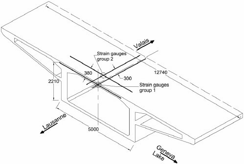
In 2016, strain gauges were glued directly on the locally exposed reinforcement bars on the bottom side of the slab. Representative location, at the viaduct centerline and middle of a typical span, was chosen. The transversal rebar response depends on the axle load, while the longitudinal rebar response is a mix of local response due to axle loads and global response due to truck weight (Sawicki & Brühwiler, 2019), thus the two are discussed here. In this paper 815 days of data registered between January 2017 and March 2020 are discussed. Data registered after introduction of lockdown in Switzerland on 13^th March 2020 is not used nor discussed due to possible lack of representativeness (Figure 1).

Figure 1. Scheme of monitoring of the highway viaduct, dimensions in mm.

3.1.1. Results of NCI

The first step in NCI method is the extrapolation of daily block maxima. One hundred one-year-long monitoring campaigns were simulated by sampling daily block maxima over the full monitoring period. Then, the return levels for return period of 75 years was extrapolated after each day of monitoring. The extrapolated values starting on January 1^st are presented in Figure 2. It can be noticed that when the amount of data is sufficient, the values are less scattered. The mean of extrapolated values after one year of monitoring is 33 µε and 132 µε for longitudinal and transversal rebars respectively, while the maximum values of strains registered during monitoring campaign were equal to 32 µε and 122 µε, respectively. Since these highest registered values are not present in every sampled dataset, it can be concluded that the number of 100 samples gives a representative mix of data. Similar behavior in terms of stabilization of value with an increase of observation time was noticed for the width of confidence interval, presented in Figure 3.

Figure 2. Extrapolated return levels for return period of 75 years for two strain gauges of the highway viaduct and the average value, 100 simulations starting on January 1^st.

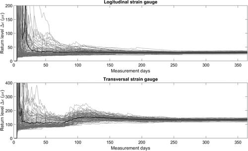
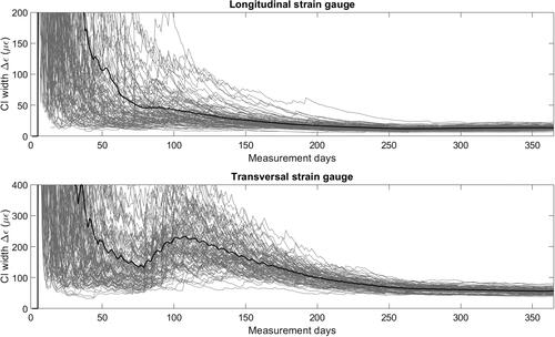
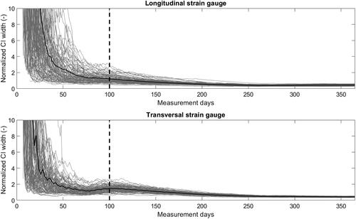
Figure 3. Confidence interval width of extrapolation of return levels for two strain gauges of the highway viaduct and the average value, 100 simulations starting on January 1^st.

The next step is to use Equations (1)(1) $$I_{\mathit{TSC},i}={\left[z_{95}-z_5\right]}_i-{\left[z_{95}-z_5\right]}_{i-1}$$(1) and (2)(2) $$I_{\mathit{NCIW},i}=\frac{{\left[z_{95}-z_5\right]}_i}{{Z75}_i}$$(2) to calculate the TSC and NCIW indicators respectively. Their values are presented in Figures 4 and 5. The TSC for longitudinal rebar stabilizes approximately after 100 days. The transverse rebar needs around 180 days to achieve stable indicator. Since the transversal rebar receives higher strains, and its response is determined by the axle load only (Sawicki & Brühwiler, 2019), this reinforcement bar is more sensitive to the traffic variability. Interestingly, the individual sampled curves reveal peaks which are spaced by 7 days. Each jump of confidence interval width is provoked by an inconsistency of new data with the previously collected. The reason is the repetitive change of daily maxima, provoked by large weekly variation of traffic. Heavily loaded trucks are observed during weekdays, while on weekends the registered daily maxima are lower. The mean NCIW is stabilizing at similar pace for both rebars. After 100 days it reaches values that are close to final, and after 180 days the final values are achieved.

Figure 4. Time Step Comparison for two strain gauges of the highway viaduct and the average value with, 100 simulations starting on January 1^st; 100 and 180 days period marked.

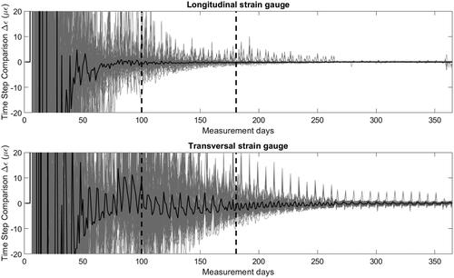
Figure 5. Normalized Confidence Interval Width for two strain gauges of the highway viaduct and the average value with, 100 simulations starting on January 1^st; 100 days period marked.

However, for individual curves this pace varies a lot for both indicators. This variability comes from the stochastic nature of traffic data. The heaviest trucks can occur in the very beginning of the monitoring campaign, leading to fast stabilization of indicators, or, they might arrive later de-stabilizing the extrapolated values. This phenomenon is discussed below.

3.1.2. Results of cumulative apparent damage

The apparent daily damage was resampled as discussed previously. The simulated curves, together with the mean value, 5^th and 95^th fractile curves are presented in Figure 6. The accumulation of damage depends on the mix of traffic present on the bridge on the given day. There is a clear seasonal variation of accumulated apparent damage, with faster growth during summer and slower during winter. This is explained by the temperature variation (Bayane et al., 2019). It was for this phenomenon that the seasons of daily damage and block maximum were kept.

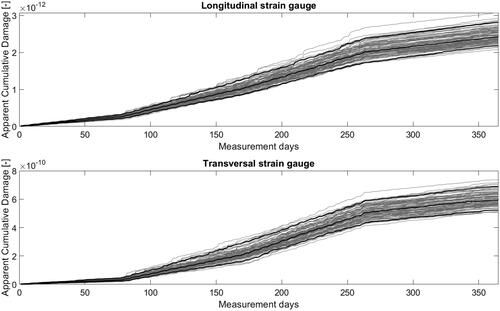
Figure 6. Apparent cumulative damage for two strain gauges of the highway viaduct and the 5^th, 50^th and 95^th fractile, 100 simulations starting on January 1^st.

As mentioned previously, the 5^th and 95^th fractiles (Figure 6) are used to calculate the γ_CDF factor. This factor is monitoring time-dependent, i.e., the shorter the monitoring duration, the higher the chance that important action effects and their combinations were omitted. Importantly, it is intended to take into account the stochastic nature of traffic only. It does not consider the seasonal variation in damage accumulation, nor it was calibrated with respect to the necessary reliability level of the structure. The values of γ_CDF factor are discussed later, taking into account data from the bi-directional road viaduct.

3.2. Bi-directional road viaduct

This viaduct was built in 1959 and is composed of seven spans of 25.6 m and an approach span of 15.8 m, with total length 195 m. The composite steel-concrete structure is located in Switzerland and carries bi-directional road traffic. The slab of variable thickness (17 cm to 24 cm) is fixed on two 1.3 m high steel box-girders. The monitoring was deployed in June 2016 (Bayane et al., 2019). Strain gauges were glued on the transverse (T1, T2) and longitudinal (L1, L2) rebars of slab, at midspan and centerline of bridge and around 70 cm from this point (see Figure 7), on spans 2 (S2) and 4 (S4).

Figure 7. Scheme of monitoring of the road viaduct; strain gauges naming: T1, T2 – transverse rebar 1 and 2; L1, L2 – longitudinal rebar 1 and 2; BG – bottom of girder.

Furthermore, one strain gauge was glued on the bottom of steel girder (BG) in longitudinal direction on span 4. Since the gauge S2T1 (transverse 1 on span 2) was not working for around 50% of monitoring duration, and gauge S4L1 (longitudinal 1 on span 4) failed soon after installation, in this paper seven strain gauges are considered. Because of expected change of traffic nature due to COVID-19 lockdown in Switzerland, the monitoring data is divided into two groups – until March 13^th 2020 when the preventive measures were introduced by the Swiss Government, and after this date. In total the presented result are prepared using 1034 full days of data registered during 44 months in pre-COVID-19 period, and 338 full days of data registered during 11 months after COVID-19 lockdown.

3.3. Before COVID lockdown

The results collected during 44 months of monitoring, between May 2016 and March 2020 were bootstrapped and analyzed as discussed previously. They are assumed to be representative for the whole service duration of the bi-directional viaduct and thus will serve as a basis for quantification of fatigue damage variation due to randomness of the traffic.

3.3.1. Results of NCI

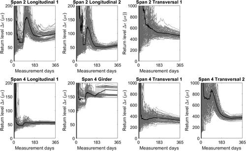
The results of extrapolation of a bootstrapped data after each day of 100 simulations starting on January 1^st are presented in Figure 8. After few days, the return level value stabilizes, to rise again around day 80 when the data collected in spring is taken into account. Due to warmer temperatures, the contribution of asphalt to the overall response of a thin reinforced concrete slab is reduced, resulting in higher measured strains. This rise is especially important in the case of gauge S4T2, and other rebars in this direction indicate similar but smaller rise in values. This can be attributed to the fact that gauge S4T2 is located directly under the wheels of passing trucks, while gauges S2T1 and S4T1 are in a certain distance, and therefore the stress due to traffic action is partially redistributed (Bayane et al., 2019) and thus less sensitive to the local variations of asphalt stiffness. The influence of temperature on structural response due to change of properties of asphalt (Watson & Rajapakse, 2000) was previously observed for a reinforced concrete bridge slabs (Hassan, Burdet, & Favre, 1993; Martín-Sanz et al., 2020). Despite these seasonal variations, the return level values after full year of monitoring are similar for all three gauges.

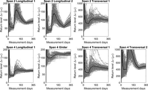
Figure 8. Extrapolated return levels for return period of 75 years for seven strain gauges of the road viaduct and the average value, 100 simulations starting on January 1^st.

Interestingly, the extrapolated return levels for three longitudinal gauges after the winter period are similar and around 50 µε, but two gauges in Span 2 (S2L1 and S2L2) indicate larger rise in values in spring and after summer months, comparing to the gauge in Span 4 (S4L1). This can be possibly attributed to different general stiffness of the two spans due to articulation axis and support stiffness (Bayane, Pai, Smith, & Brühwiler, 2021), but impossible to verify using the discussed monitoring scheme.

The variation of the extrapolated return level based on the strain gauge installed on girder (S4BG) is the smallest. This is because the two possible phenomena governed by the stiffness of asphalt: modification of slab inertia and distribution of wheel load, do not affect the longitudinal steel structure. The contribution of asphalt to the bridge inertia in longitudinal direction is negligible, since most of stiffness comes from girders and reinforced concrete. Furthermore, the reduced capabilities of wheel load distribution is not affecting the steel girder as there is no direct action of traffic imposed on it. The above confirms therefore that it is a local response that changes with the temperature variation, rather than the global behavior of structure.

The mean extrapolated return levels after 365 days and the measured maximum values for each gauge are presented in Table 1. For all strain gauges glued on rebars the extrapolated values are higher than measured, indicating scatter of obtained results and thus sensitivity to the traffic variation. The scatter can be qualitatively assessed by the difference between maximum measured value and extrapolated value, in the current case varying between 10% and 25%. Comparing to the highway viaduct (3% and 7%) this difference is larger probably due to the influence of asphalt as discussed previously. However, in case of the strain gauge installed on the steel girder (S4BG), the extrapolated value is even slightly smaller (3%) than the maximum measurement, indicating uniform monitoring results with some isolated events which are not drafted for certain permutations. Values of the confidence interval width are presented in Figure 9. For all sensors, except for the one installed on girder, the stabilization occurs much later than in case of the highway viaduct, especially for gauges S2L1, S2L2 and S4T2. In case of the strain gauge installed on girder, a stable and narrow confidence interval is reached around day 70.

Figure 9. Confidence interval width of extrapolation of return levels for seven strain gauges of the road viaduct and the average value, 100 simulations starting on January 1^st.

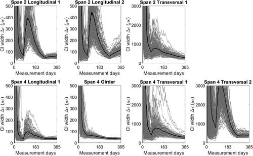
Table 1. Comparison of maximum measured values of strain and return levels extrapolated after 365 days starting January 1^st for the road viaduct before COVID-19 lockdown.

Strain gauge	S2L1	S2L2	S2T1	S4L1	S4BG	S4T1	S4T2
Maximum measured value Δε (με)	83	57	445	64	180	389	372
Mean return level after 365 days Δε (με)	97	93	499	73	175	434	501

Figure 10 presents the time step comparison (TSC) and Figure 11 the normalized confidence interval width (NCIW) for all gauges of bi-directional road viaduct starting on January 1^st. Around day 100 there is a clear rise of all indicators due to change of seasons as discussed previously. Strain gauges S2T1, S4L1, S4T1 and S4GB present a quick pace of decrease of indicators’ values. In all cases the values of indicators after day 100 are decreasing and, except for transverse rebars, values similar to those observed for the previously discussed highway viaduct are reached after 180 days or earlier. The values of TSC indicator for transverse gauges are one magnitude larger than for other gauges. This cannot be observed for NCIW, which is normalized with respect to the return value. Therefore, the large gap between TSC values for rebars in two directions can be attributed to difference in magnitude of measured values of strain ranges, and consequently extrapolated return values and associated widths of confidence intervals.

Figure 10. Time Step Comparison for seven strain gauges of the road viaduct and the average value with, 100 simulations starting on January 1^st; 100 and 180 days period marked.

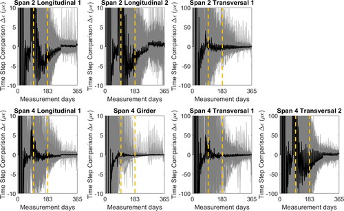
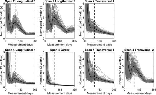
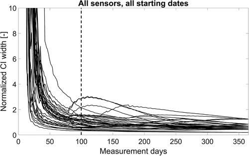
Figure 11. Normalized Confidence Interval Width for seven strain gauges of the road viaduct and the average value with, 100 simulations starting on January 1^st; 100 days period marked.

3.3.2. Results of cumulative apparent damage

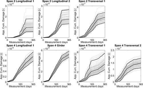
The bootstrapped apparent cumulative damage for the bi-directional road viaduct starting on January 1^st is presented in Figure 12. Very large increase of damage accumulation is visible in spring and summer due to the abovementioned contribution of asphalt layer, except for the girder. Since the strain variation in transversal reinforcement bars is larger than in longitudinal direction, and the number of cycles is associated with axles passes rather than trucks pass, the apparent accumulated damage is two orders of magnitude larger as well. The accumulated fatigue damage between each rebar in the respective direction varies largely, proving that proper placing of sensors is crucial for successful and informative monitoring campaign (Bertola, Proverbio, & Smith, 2020).

Figure 12. Apparent cumulative damage for seven strain gauges of the road viaduct and the 5^th, 50^th and 95^th fractile, 100 simulations starting on January 1^st.

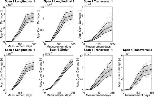
For transversal reinforcement bars 1 on both spans (S2T1 and S4T1), a rapid increase of 95% fractile values compared to 5% fractile can be noticed. This is due to few isolated days in autumn, which for this starting date is towards the end of bootstrapping period, when the high strain variation and number of cycles was registered, bringing considerably large amount of damage. These events get resampled for some permutations, while not for the others. The effect of this overloading is less visible for sensor S4T2, and not at all in longitudinal direction. This is because the transversal reinforcement is much more sensitive to single axle loads, while in the longitudinal direction the overall loading is more important. After discussing with the road owner it was concluded that the large accumulation of damage occurred during few days when construction works were taking place on a nearby road, and a large amount of aggregate was transported by heavily loaded trucks. This kind of events can alter the obtained results and need to be taken into account while planning short-term monitoring campaigns.

3.4. During and after COVID lockdown

Since the COVID-19 lockdown lead to temporary halt of economic activity and almost complete lack of road traffic, it is expected that the results obtained by the monitoring are not representative. To verify this assumption, data collected between introduction of preventive measures by the Swiss government (13.03.2020) and the end of the monitoring campaign (14.02.2021) are treated separately in the same way as discussed above. Since the amount of data is much smaller compared to the pre-lockdown period, and shorter than one year, shuffling with repetition was used.

3.4.1. Results of NCI

The extrapolated return level on the basis of 11 months of monitoring during and after COVID-19 lockdown is presented in Figure 13. Large scatter of obtained values is visible especially for S4BG gauge. This is due to an isolated event registered on September 3^rd 2020, when a strain of 183µε was measured, being 20% larger than the second largest daily maximum of this period. It is however comparable with the largest strain recorded in the pre-covid period by this gauge (180µε). An elevated peak, although not the largest one, is visible on the given day for transversal rebars on the discussed span 4, albeit not on longitudinal. It is probably produced by an unfortunate position of a heavily loaded truck on the viaduct, and cannot be considered as an outlier. Since shuffling with repetitions is used here, this isolated event is drafted for some cases multiple times, while not at all for the others. Furthermore, it occurs in autumn which is close to the end of a year-long monitoring period for a given starting date. Therefore, two groups of datasets are formed, with return levels around 155µε and 185µε.

Figure 13. Extrapolated return levels for return period of 75 years after COVID-19 lockdown for seven strain gauges of the road viaduct and the average value, 100 simulations starting on January 1^st.

The extrapolated return levels after one year in comparison with the previously discussed results can serve for quantification of representability of the data collected during that period. The maximum measured values in this period and the extrapolated return levels after 365 days are presented in Table 2. While comparing with Table 1 it cannot be stated unambiguously that there exists a large difference between the two monitoring periods. All return levels are larger than the maximum measured values except for S4BG gauge, due to an isolated event on 03.09.2020 as discussed before. Since the daily maxima are compared here, it can be concluded that the weight of heaviest trucks did not change in the period considered. The TSC and NCIW will not be discussed as not enough data is available.

Table 2. Comparison of maximum measured values of strain and return levels extrapolated after 365 days starting January 1^st for the road viaduct after COVID-19 lockdown.

Strain gauge	S2L1	S2L2	S2T1	S4L1	S4BG	S4T1	S4T2
Maximum measured value Δε (με)	90	46	388	53	183	317	323
Mean return level after 365 days Δε (με)	99	58	465	56	173	324	375

3.4.2. Results of cumulative apparent damage

The apparent cumulative damage bootstrapped on the basis of data collected after COVID-19 lockdown in Switzerland (13.03.2020) is presented in Figure 14. Considerably large scatter of values is observed due to drafting with repetitions. Comparing to the pre-lockdown results (Figure 12) the mean values are similar for sensors S2L2, S2T1 and S4GB. For all other strain gauges except of S2L1 the results are much smaller. Interestingly, in case of gauge Span 2 Longitudinal 1 the obtained means value is more than one order of magnitude larger, with rapid increase in summer. No valid explanation for this large difference was found.

Figure 14. Apparent cumulative damage after COVID-19 lockdown for seven strain gauges of the road viaduct and the 5^th, 50^th and 95^th fractile, 100 simulations starting on January 1^st.

The above observations, together with daily maxima values already discussed, can lead to the conclusion that the number of heavily loaded trucks slightly decreased. However, it can be stated that the lockdown period did not significantly influence collected monitoring data. Still, the data collected after 13.03.2020 is not take into account for discussion of monitoring duration and extrapolation methods.

4. Discussion

The data from the two viaducts was resampled and processed as discussed previously, using all available sensors and four starting dates. The general results taking into account mean values of NCI indicators and γ_CDF calculated for each set of 100 permutations for each gauge on a given starting day are presented in this section. As mentioned previously, only data collected before COVID-19 lockdown in Switzerland (13^th March 2020) was used.

4.1. Minimum monitoring duration

The mean Time Step Comparison and Normalized Confidence Interval width for all sensors are presented in Figures 15 and 16, respectively. For most of the sensors, the stabilization occurs before 100 days of monitoring. In certain cases, the indicators are rising after some monitoring time. These are rebars of the bi-directional road viaduct. As discussed, since the reinforced concrete slab is relatively thin, the contribution of asphalt pavement to the structural response is important, leading to large variation of structural response depending on the temperature. Thus, the strains registered in summer are higher than those registered in winter.

Figure 15. Time Step Comparison for nine gauges of both viaducts, 100 simulations starting on four seasons; 100 days period marked.

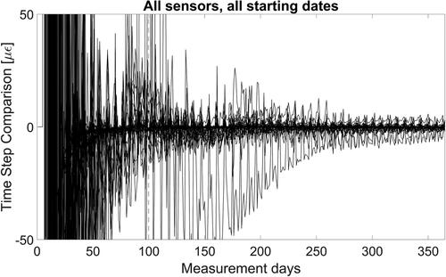
Figure 16. Normalized Confidence Interval Width for nine gauges of both viaducts, 100 simulations, four starting days; 100 days period marked.

The effect of this phenomenon is most visible for simulations starting in winter (January 1^st). After the period of measurements during winter and spring, TSC and NCIW indicators stabilize. Indeed, the TSC for S4T2 gauge of the road viaduct, with bootstrapping starting on January 1^st, reaches values below −50 με around day 100, and joins the other sensors only around day 250. It is represented by the lowermost curve in Figure 15. For this gauge and starting date, similar situation takes place for NCIW indicator (Figure 16) – it is the uppermost curve around day 100.

However, the two other maxima of NCIW around day 100 are reached by gauges S2L1 and S2L2, with bootstrapping starting on January 1^st. It is therefore clear that they are affected by asphalt contribution as well, as discussed previously on the basis of respective confidence interval widths presented in the Figure 9. Furthermore, since the measured strains are relatively lower than in the transversal direction, the NCIW is more sensitive to changes. It is to that extend that in case of gauge S2L2 and simulation starting in July, the NCI indicator rises around day 90 (beginning of autumn) and starts decreasing only around day 170 (beginning of winter), after reaching the value of 2.3.

The presented methods provide reliable results only for stationary data in terms of not only traffic loading, but the temperature as well. However, it can be concluded that if the effect of temperature is taken into account otherwise or it is not important, the minimum monitoring time to capture the traffic data reliably is around 100 days. This confirms findings by (Treacy et al., 2014) as obtained from a monitoring campaign of a reinforced concrete highway viaduct.

4.2. Optimal monitoring duration and correction factor

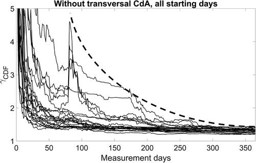
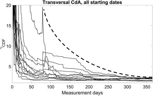
The daily apparent damage was resampled and treated as described previously. Since the response of the transversal reinforcement bars of the road viaduct is very sensitive to temperature variation, they are discussed separately. Figure 17 presents the values of Cumulative Damage correction Factor γ_CDF prepared on the basis of resampling of accumulated damage for six strain gauges (transversal and longitudinal rebars of the highway viaduct; longitudinal rebars and box-girder of the road viaduct). For most of the sensors, the value of γ_CDF stabilizes around the 50^th measurement day. There are two curves with visible peaks around day 70. These are gauges on longitudinal rebars of the road viaduct, which registered an extremely heavy truck passage. Nevertheless, the factor reached the value of 4.0 only. Overall, the value of γ_CDF factor after full year of monitoring is 1.3. The dashed curve in Figure 17 presents proposed time-variation of γ_CDF to be applied to monitoring results of massive reinforced concrete or composite structures not sensitive to temperature effects.

Figure 17. Cumulative Damage correction Factor γ_CDF based on seven gauges (not taking into account transversal rebars of the road viaduct) and four starting dates; curve of proposed γ_CDF values marked with dashed line.

In the case of transversal rebars of the road viaduct, which are highly sensitive to temperature, the convergence rate of the γ_CDF factor depends on the starting date of simulation (Figure 18). The results are destabilized, which was discussed previously. Still, the value of γ_CDF factor after full year of monitoring is below 2.5 in all cases, which is considerably lower than the factor of 20 proposed in Eurocode (EC1.,1, 2003). The dashed curve presents proposed γ_CDF for temperature sensitive elements.

Figure 18. Cumulative Damage correction Factor γ_CDF based on three gauges (transversal rebars of the road viaduct) and four starting dates; curve of proposed γ_CDF values marked with dashed line.

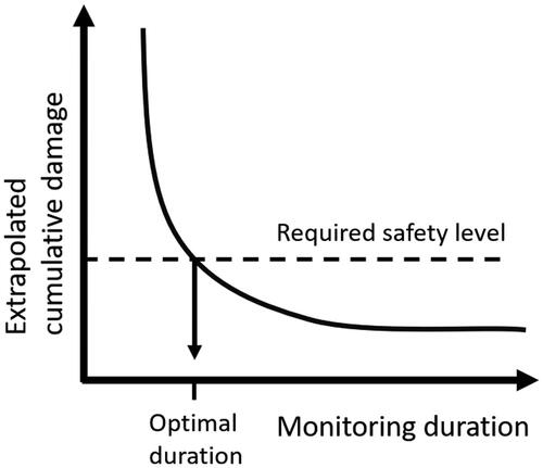
Using the developed Cumulative Damage correction Factor γ_CDF, the case-specific optimum monitoring duration can be found. With longer duration, the resulting extrapolated cumulative damage is reduced as presented schematically in Figure 19. Once the required level of extrapolated cumulative damage, i.e., structural safety, is achieved, the monitoring can be terminated. In this way, the monitoring campaign takes as long as necessary, and the monitoring resources (e.g., data acquisition systems) can be optimally allocated among structures under surveillance.

Figure 19. Schematic presentation of optimal monitoring duration concept.

5. Conclusions

Long term monitoring data from two viaducts was analyzed and resampled to investigate the minimum monitoring time required to capture with sufficient reliability the nature of road traffic loading. The method to take into account uncertainty due to short duration of observation in the cumulative damage approach is proposed as well. This Cumulative Damage correction Factor does not take into account possible future increase in traffic and may vary if other types of S-N curves are applied. Accordingly, the following conclusions can be drawn:

• The minimum monitoring duration for road bridges is 100 days; if the monitoring is shorter, the collected data cannot be considered as reliable.

• Since the structural response can be highly dependent on ambient temperature, the recommended season to conduct short-term monitoring is during summer months with high temperatures.

• Possible seasonal variation of traffic must be taken into account in the planning of short-term monitoring; however, the two case studies did not reveal such variation. Nevertheless, isolated events during short-term monitoring can alter the results.

• Using the resampled data, the Cumulative Damage correction Factor γ_CDF is proposed. It takes into account variation of the road traffic and lack of representability of results of short-term monitoring campaign, while using them in extrapolation of cumulative fatigue damage.

• For most cases, the Cumulative Damage correction Factor of γ_CDF=4 is suggested for cumulative damage extrapolation after 100 days of monitoring, and γ_CDF=1.3 after 1 year.

• For structures highly sensitive to temperature variation, γ_CDF=20 (or Eurocode method) should be used for accumulated damage after 100 days of monitoring and γ_CDF=2.5 for 1 year-long monitoring; to reduce these values, longer monitoring can be considered.

• The COVID-19 lockdown did not significantly alter the measured values of strain and accumulated apparent fatigue damage.

Acknowlegements

This project has received funding from the European Union’s Horizon 2020 research and innovation program under the Marie Skłodowska-Curie grant agreement No 676139.

Disclosure statement

No potential conflict of interest was reported by the authors.

References

- Ahmadivala, M., Sawicki, B., Brühwiler, E., Yamalas, T., Gayton, N., Mattrand, C., & Orcesi, A. (2019). Application of time series methods on long-term structural monitoring data for fatigue analysis. In SMAR 2019 Programme and Downloads. Retrieved from https://infoscience.epfl.ch/record/270411.
- ASCE. (2017). 2017 infrastructure report card. Retrieved from https://www.infrastructurereportcard.org/cat-item/bridges/.
- Bayane, I., Mankar, A., Brühwiler, E., & Sørensen, J. D. (2019). Quantification of traffic and temperature effects on the fatigue safety of a reinforced-concrete bridge deck based on monitoring data. Engineering Structures, 196, 109357. doi:10.1016/j.engstruct.2019.109357
- Bayane, I., Pai, S. G. S., Smith, I. F. C., & Brühwiler, E. (2021). Model-based interpretation of measurements for fatigue evaluation of existing reinforced concrete bridges. Journal of Bridge Engineering, 26(8), 04021054. doi:10.1061/(ASCE)BE.1943-5592.0001742
- Bertola, N. J., Proverbio, M., & Smith, I. F. C. (2020). Framework to approximate the value of information of bridge load testing for reserve capacity assessment. Frontiers in Built Environment, 6. doi:10.3389/fbuil.2020.00065
- Brühwiler, E. (2017). Learning from the past to build the future, Editorial. Proceedings of the Institution of Civil Engineers - Engineering History and Heritage, 170(4), 163–165. doi:10.1680/jenhh.2017.170.4.163
- Brühwiler, E., Bastien-Masse, M., Mühlberg, H., Houriet, B., Fleury, B., Cuennet, S., … Maurer, M. (2015). Strengthening the Chillon viaducts deck slabs with reinforced UHPFRC. IABSE Symposium Report, 105, 1–8. doi:10.2749/222137815818358457
- Chen, S.-Z., Wu, G., & Feng, D.-C. (2019). Damage detection of highway bridges based on long-gauge strain response under stochastic traffic flow. Mechanical Systems and Signal Processing, 127, 551–572. doi:10.1016/j.ymssp.2019.03.022
- Crespo-Minguillón, C., & Casas, J. R. (1998). Fatigue reliability analysis of prestressed concrete bridges. Journal of Structural Engineering, 124(12), 1458–1466. doi:10.1061/(ASCE)0733-9445(1998)124:12(1458)
- EC1. (2003). EN 1991-2: Eurocode 1: Actions on structures - Part 2: Traffic loads on bridges. Retrieved from http://archive.org/details/en.1991.2.2003.
- Flanigan, K. A., Lynch, J. P., & Ettouney, M. (2020). Probabilistic fatigue assessment of monitored railroad bridge components using long-term response data in a reliability framework. Structural Health Monitoring, 19(6), 2122–2142. doi:10.1177/1475921720915712
- Hassan, M., Burdet, O., & Favre, R. (1993). Interpretation of 200 Load Tests of Swiss Bridges. Remaining Structural Capacity. IABSE Report, 67, 319–326. doi:10.5169/seals-51390
- Herwig, A. (2008). Reinforced concrete bridges under increased railway traffic loads [PhD thesis]. EPFL. doi:10.5075/epfl-thesis-4010
- ISO 13822. (2010). ISO 13822:2010(en), Bases for design of structures—Assessment of existing structures. International Organisation for Standardization. Retrieved from https://www.iso.org/obp/ui/#iso:std:iso:13822:ed-2:v1:en:sec:I.
- Kromanis, R., & Kripakaran, P. (2016). SHM of bridges: Characterising thermal response and detecting anomaly events using a temperature-based measurement interpretation approach. Journal of Civil Structural Health Monitoring, 6(2), 237–254. doi:10.1007/s13349-016-0161-z
- Leander, J. (2010). Improving a bridge fatigue life prediction by monitoring. Licentiate, KTH, School of Architecture and the Built Environment (ABE), Civil and Architectural Engineering, Structural Design and Bridges. Retrieved from http://urn.kb.se/resolve?urn=urn:nbn:se:kth:diva-28618.
- Li, Z. X., Chan, T. H. T., & Ko, J. M. (2001). Fatigue analysis and life prediction of bridges with structural health monitoring data — Part I: Methodology and strategy. International Journal of Fatigue, 23(1), 45–53. doi:10.1016/S0142-1123(00)00068-2
- Lipari, A., O’Brien, E. J., & Capriani, C. C. (2012). A comparative study of a bridge traffic load effect using micro-simulation and Eurocode load models. In Biondini F, & Frangopol DM (Eds.), Bridge maintenance, safety, management, resilience and sustainability (pp. 3420–3427). London: CRC Press. Retrieved from https://researchrepository.ucd.ie/handle/10197/7162.
- Martín-Sanz, H., Tatsis, K., Dertimanis, V. K., Avendaño-Valencia, L. D., Brühwiler, E., & Chatzi, E. (2020). Monitoring of the UHPFRC strengthened Chillon viaduct under environmental and operational variability. Structure and Infrastructure Engineering, 16(1), 138–168. doi:10.1080/15732479.2019.1650079
- Nilimaa, J., Bagge, N., Häggström, J., Blanksvärd, T., Sas, G., Täljsten, B., & Elfgren, L. (2016). More realistic codes for existing bridges. In Challenges in Design and Construction of an Innovative and Sustainable Built Environment, p. 9.
- Olofsson, I., Elfgren, L., Bell, B., Paulsson, B., Niederleithinger, E., Jensen, J. S., … Bien, J. (2005). Assessment of European railway bridges for future traffic demands and longer lives – EC project “Sustainable Bridges”. Structure and Infrastructure Engineering, 1(2), 93–100. doi:10.1080/15732470412331289396
- Plos, M., Gylltoft, K., Lundgren, K., Elfgren, L., Cervenka, J., Bruhwiler, E., … Rosell, E. (2006). Structural assessment of concrete railway bridges: Non-linear analysis and remaining fatigue life. In Advances in bridge maintenance, safety management, and life-cycle performance, set of book & CD-ROM (Vol. 1–0, pp. 741–744). London: CRC Press. doi:10.1201/b18175-314
- Sawicki, B., & Brühwiler, E. (2019, August). Long term monitoring of a UHPFRC-strengthened bridge deck slab using strain gauges. SMAR 2019. In 5th International Conference on Smart Monitoring, Assessment and Rehabilitation of Civil Structures, Potsdam, Germany. Retrieved from https://infoscience.epfl.ch/record/270410.
- Sawicki, B., & Brühwiler, E. (2020). Long-term strain measurements of traffic and temperature effects on an RC bridge deck slab strengthened with an R-UHPFRC layer. Journal of Civil Structural Health Monitoring, 10(2), 333–344. doi:10.1007/s13349-020-00387-3
- Schläfli, M., & Brühwiler, E. (1998). Fatigue of existing reinforced concrete bridge deck slabs. Engineering Structures, 20(11), 991–998. doi:10.1016/S0141-0296(97)00194-6
- SIA 262. (2014). Swiss standard SIA 262:2014 Concrete Structures.
- SIA 269. (2011). Swiss standard SIA 269:2011 Existing structures—Bases.
- SIA 269/2. (2011). Swiss standard SIA 269/2:2011 Existing structures—Concrete structures.
- Treacy, M. A., & Brühwiler, E. (2015). Action effects in post-tensioned concrete box-girder bridges obtained from high-frequency monitoring. Journal of Civil Structural Health Monitoring, 5(1), 11–28. doi:10.1007/s13349-014-0097-0
- Treacy, M. A., Brühwiler, E., & Caprani, C. C. (2014). Monitoring of traffic action local effects in highway bridge deck slabs and the influence of measurement duration on extreme value estimates. Structure and Infrastructure Engineering, 10(12), 1555–1572. doi:10.1080/15732479.2013.835327
- Wang, J. Y., Ni, Y. Q., & Ko, J. M. (2003). Local damage detection of bridges using signals of strain measurements. In Proceedings of the 1st International Conference on Structural Health Monitoring and Intelligent Infrastructure. Retrieved from http://hdl.handle.net/10397/56837.
- Watson, D. K., & Rajapakse, R. (2000). Seasonal variation in material properties of a flexible pavement. Canadian Journal of Civil Engineering, 27(1), 44–54. doi:10.1139/l99-049
- Zhao, G., Fu, C. C., Lu, Y., & Saad, T. (2018). Fatigue assessment of highway bridges under traffic loading using microscopic traffic simulation. In Zhou YL, & Wahab MA (Eds.), Bridge optimization—inspection and condition monitoring. London: IntechOpen. doi:10.5772/intechopen.81520