Analytical model of multiview autostereoscopic 3D display with a barrier or a lenticular plate

ABSTRACT

A geometric model of an autostereoscopic 3D display is described herein. This model is based on the geometry of typical display devices and on the projective transformations that provide periodicity in the projective space. The formulas for the transformations between regions and spaces are provided. The model can be applied to the study of an operation of the multiview, integral, plenoptic, and light-field displays. A practical application considered in this paper is the multiview wavelet transform.

KEYWORDS:

• Analytical model
• autostereoscopic display
• multiview wavelet
• integral imaging
• plenoptic imaging

View correction statement:

Correction

1. Introduction

There are several types of the autostereoscopic three-dimensional (3D) devices known: multiview displays, plenoptic displays, and integral imaging displays (sensors) (see [1–5] and the references therein). In these devices, the content of the image plane can be treated as a two-dimensional (2D) representation of a photographed/ computer-generated 3D scene. Depending on the device type, this image is called differently: a multiview image [6], an integral image [7,8], a light-field image [9], or a plenoptic image [10]. Some plenoptic cameras are already available in the market [11,12].

Despite the taxonomic difference between the mentioned autostereoscopic devices and methods, the structure of the image in the image plane of all the mentioned devices is the same or very similar [13]; basically, it consists of repeated image cells spread across the whole image. The similarity between the multiview images and the integral images [13–15] (confirmed in [14] in numerical experiments) allows the description of an integral image in terms of the multiview image, and vice versa. The structure of the plenoptic image is similar to that of the integral image [16]. Therefore, the image in the image plane of all the three types will be called ‘composite multiview image,’ without paying particular attention to the difference. A cell of a composite image has some small patches from different parallaxes [17].

The multiview image can be composed from separate view images [18], as well as decomposed into a set of images [19]. In the case of a digital screen, the number of view images (parallaxes) is equal to the number of pixels in the image cell [19]. For instance, in multiview displays, the number of pixels in a cell is usually about 10, but in super-multiview displays, this number can reach and even exceed a hundred.

The above similarity makes it possible to consider various 3D displays from a common point of view. Today, however, there are only a few models of autostereoscopic devices that are known [20,21], each depicting a particular feature of a 3D display. Useful geometric relationships are given in [22] and [23]. The model in [24] describes a recording system using a hexagonal array of microlenses, including many useful formulas and expressions for the disparity and the spread function. The paper [21] provides a model based on a homogeneous matrix describing the range of perceived distances, including the limitation due to stereopsis (fusion). Stern and Javidi [25] classify the integral displays and analyze an ideal display. [22] is based on the lens model. In [26] and [27], the viewing angle, range, and angular resolution are analyzed. Plenoptic imaging is analyzed in [28] and [29]. None of the above-mentioned works on 3D imaging, however, presents a systematic model of a whole multiview display.

From the authors’ point of view, geometry is one of the most fundamental system properties, whose influence on the quality cannot be neglected. The equivalence of the light sources, pinholes, and lenses is explained in [23]. Therefore, the term ‘point source’ is used in the model even if a device actually uses lenses or pinholes.

Although the analytical formulation was made relatively recently in [30] and [31], some important properties of multiview images were already used in the multiview stereograms [32] in 1999, and some aspects of the model have been occasionally mentioned and have already been used, particularly in [14], [33], and [34].

The proposed analytical model is based on the most typical structure and on most of the general geometric properties of autostereoscopic displays, and therefore covers a wide range of autostereoscopic displays and sensors. The model allows finding various geometric parameters of the autostereoscopic 3D display analytically, in a convenient closed form. An essential part of the model is the projection transformation. The discrete planes in the projected regions are equidistant (an essential feature of the projection model). A particular advantage of the projective form is in the uniform layout of regions; therefore, wider areas of regions can be observed at once. This makes the model a useful and flexible tool for various practical applications, including for the measurements of the optimal viewing distance (OVD) [35] and the estimation of the image quality [33] and wavelet transform [36].

The paper is organized as follows. First, in Section 2, the autostereoscopic 3D display device in the regular Cartesian space is described, and the layout of the image and object regions as well as the screen cells, quasi-horizontal cross-sections, converging/diverging geometry, sites, depth planes, and multiple regions are presented. Second, in Section 3, the projections, plane-to-plane transform, multiple projected regions, and spatial structure are discussed. Third, in Section 4, the multiview wavelets are introduced as a logical consequence of Section 3. Finally, the Discussions and Conclusions sections end the paper.

2. Basic definitions and objects of the model

2.1. Light sources and observer

A plain 2D array (matrix) of point light sources is installed orthogonally to the line of sight. All the light sources in matrix a are identical, have identical brightness, and emit light within a certain cone around their axes. The array consists of horizontal lines, a_i being one of them. The currently visible light source for each eye is selected by the modulation screen s (see Figure 1).

Figure 1. General layout of a typical autostereoscopic 3D display (main items of the geometric description).

The best image is seen from within horizontal line segment b (the observer base), which is parallel to a. Observer base b is sometimes called a ‘sweet spot.’ Screen s is located between the array of light sources and the base. The physical meanings of a, b, and s, however, are different: whereas a and s represent physical bodies (the light source array and the screen), b is just a pre-defined location in front of the screen.

The parallel lines a_i and b lie in a certain plane P_i (see Figure 1). Distance d between observer base b and the array of light sources a is called the ‘OVD.’ The origin is located at the intersection of the diagonals of the isosceles trapezoid with the bases a_i and b. Distances d_a and d_b are the distances from the origin to lines a_i and b.

Although lines a_i and b are horizontal, plane P_i may not be horizontal. Therefore, it will be more accurate to call plane P_i ‘almost horizontal’ or ‘quasi-horizontal.’

2.2. Screen

A multiview autostereoscopic 3D display device, as a rule, consists of two parallel layers: the first layer is the array of light sources, and the second layer is the modulation screen (see Figure 1). The screen s displays a specially prepared composite multiview image.

Instead of the light sources formally considered in the model, their optical equivalents within the framework of the linear geometric optics can be used in practice. For example, lenses or pinholes can be used with a few differences, in almost the same manner. Correspondingly, a transparent screen is combined with the array of physical light sources, and a light-emitting screen is combined with the array of lenses (or pinholes).

The screen of an autostereoscopic 3D display can be regarded as consisting of logical cells, with one cell per light source. The cell is a part of the screen. The corresponding cell is defined as the cell through which the light ray from the light source passes to the center of base b.

The layout of the cells directly corresponds to the layout of the light sources [30,37]. The shape of the screen is geometrically similar to the shape of the array. With a uniform array of light sources, all the cells are identical and thus could be either squares (rectangles, parallelograms, or rhombi) or hexagons.

2.3. Regions

In the space around a 3D autostereoscopic 3D display device, two fundamental spatial volumes can be brought out: where the images are displayed and where the images are observed. These volumes are referred to as the image region and the observer region.

The observer region is located in front of the display screen, around the base. From the base, the image is perceived without visual crosstalk. From the central (main) observer region, all the light sources (each and every light source, without any exception) are seen through the corresponding cells.

Figure 2. Image region (dotted line) and observer region (dashed line).

The image region is a volume for locations potentially seen by an observer at base b. It is a functional analogue of the viewing frustum in 3D computer graphics. The image region occupies the array of light sources: the screen together with the adjacent space in front and behind them.

The cross-section of regions lying in a quasi-horizontal plane P_i is shown in Figure 2. The region is shaped like a deltoid (kite), a symmetric quadrilateral consisting of two adjacent isosceles triangles. Base b and array a_i are the main diagonals of the corresponding regions.

The ratio of the horizontal size (width) of the array of light sources to the width of the observer’s base determines the principal characteristic of the geometry of the multiview display device. (1) $c=\frac{b}{a},$(1) where a and b are defined above, in Section 2.1.

When c > 1, the geometry is converging; otherwise, it is diverging. As the sides of the regions are extensions of the same two rays, only one region is closed (finite); the other is open (infinite), as can be seen in Figure 2.

2.4. Sites

Observer base b is divided into n segments, often called ‘viewing zones’; n is equal to the number of parallaxes N_v (view images) corresponding to the specific position and direction of the camera when the image was photographed or synthesized. In displaying, each of the segments receives an image of one parallax. In multiview displays, there are typically a few segments per interocular distance (approx. 6.5 cm). In super-multiview displays [38], the segments are short as their length is essentially smaller than the interocular distance and can be even less than the diameter of the pupil of the human eye.

Similarly, the main diagonal a of the image region is divided into m segments (m = N*−1), where N* is the number of light sources along one row of the matrix.

The geometric structure and other properties of regions [39] are basically defined by the rays from the light sources to the segments of the base. By these rays, the regions are divided into a number of subregions [40,41] (see Figure 3).

Figure 3. Rays across two regions, sites, and depth planes for (a) four light sources (c > 1, N_v = 1, N* = 4) and (b) four views (c < 1, N_v = 4, N* = 2).

The rays of two minimal layouts (in the first, N* light sources are combined with one parallax, while in the second, two light sources are combined with n parallaxes) define quadrilateral subregions called ‘sites’ herein (see Figure 3). Due to their special meaning, the intersections of the rays of the minimal layouts are sometimes called ‘nodes.’ In the case of the first minimal layout (one parallax), there are m² sites in the image region; in the case of the second minimal layout (two light sources), there are n² sites in the observer region (Figure 3).

2.5. Discrete depth planes

The main diagonals of the sites (which are parallel to the array of light sources) can be merged together and form a set of discrete lines l_i, where i = 0, 1, … , 2n for the image region, and i = 0, 1, … , 2 m for the observer region (see Figure 3). They will be called ‘depth lines’ because they are cross-sections of the depth planes. These lines are sometimes called ‘nodal lines’ [30]. The depth planes were considered in [17] and [42].

The 0th depth line of both regions coincides with the x-axis. The nth depth line of the observer region is observer base b, while the mth depth line of the image region is the array of light sources. The 2nth and 2mth lines are at the farthest apexes of the regions.

2.6. Analytical formulas

A formula for the location of the depth line can be obtained from geometric considerations, as follows. The similar triangles of two kinds (with sides a and b and an intermediate i-th depth line; see Figure 3(a)) imply that (2) $\frac{m{w}_i}{a}=\frac{d_b+l_i}{d},$(2) and (3) $\frac{i{w}_i}{b}=\frac{l_i}{d_b},$(3) where d_b is the distance between the observer base and the origin. (4) $d_b=\frac{1}{1+c^{-1}}d=\frac{c}{1+c}d.$(4) Excluding w_i from Equations (2) and (3), (5) $\frac{b}{i}\frac{l_i}{d_b}=\frac{a}{m}\frac{d_b+l_i}{d},$(5) and substituting the definitions of c and d_b from Equations (1) and (4), the equation below is obtained. (6) $m{l}_i=i\frac{1}{1+c}(d_b+l_i)$(6) Isolating the terms with l_i in Equation (6), the formula for the location of the depth line l_a is obtained.

(7) $l_a\left(i\right)=\frac{i}{f_a\left(i\right)}{d}_b=\frac{i}{f_a\left(i\right)}\cdot \frac{c}{1+c}d,$(7) where (8) $f_a\left(i\right)=m(c+1)-i.\left(8\right)$(8) The formulas for other important geometric characteristics of the image region, such as the distance between the successive depth lines Δl_a and the width of the sites w_a, are derived from Equation (7), as shown below (these quantities are graphically shown in Figure 3).

(9) $\mathrm{\Delta }{l}_a\left(i\right)=l_a(i+1)-l_a\left(i\right)=\frac{mc}{f_a\left(i\right)\left(f_a\right(i)-1)}d,$(9) (10) $w_a\left(i\right)=\frac{1}{f_a\left(i\right)}b.$(10) Equation (4) represents the location of the base (the distance to the origin) shown in Figure 1, while Equation (8) defines a function that is common for many expressions, such as Equations (7), (9), and (10). This function characterizes the region.

Note that the subscript b means the observer region while the subscript a relates to the image region.

2.7. Location of the screen

Although the screen can generally be located anywhere between the array of light sources and the base, it is typically located at the discrete plane adjacent to the main diagonal of the image region: either the (m − 1)-th or the (m + 1)-th discrete plane. At these planes, the screen area is used most efficiently, without gaps and overlaps. The formulas for the screen are available in [30] and [42]. The screen at the (m − 1)-th line is a transparent screen combined with the physical light sources at a, while the screen at the (m + 1)-th line is a light-emitting screen combined with the lens array or pinhole array at a (see Figure 4). The images of these cases can be easily transformed into each other [43].

Figure 4. Screen (two options) (N_v = 1, N* = 4).

In the case of the lens array, as a rule, the distance between the lens array and the array of light sources coincides with the focal length of the lenses, although this is not a requirement. This condition is not satisfied in the modified integral photograph [44].

2.8. Correspondence between two regions

The formulas for the observer region were obtained in [45]. The picture of the regions, sites, and discrete planes (Figure 3) suggests a similarity between the regions; as such, the analytical descriptions of the regions should be similar. Therefore, in principle, it is sufficient to consider only one region; the description of another region can be based on the similarity (i.e. the changes in the variables), (11) $\begin{array}{rl}a& \leftrightarrow b,\\ m& \leftrightarrow n,\\ x& \leftrightarrow -x,\\ z& \leftrightarrow -z,\end{array}$(11) and consequently, (12) $c\leftrightarrow c^{-1};$(12) this converts the formulas for one region to the formulas for another.

The above correspondence creates an interchangeability of the analytical descriptions of the regions. The formulas for the observer region are obtained by applying the rules in Equations (11) and (12) to Equations (7)–(10). The result is as follows: (13) $l_b\left(i\right)=\frac{i}{f_b\left(i\right)}{d}_a=-\frac{i}{f_b\left(i\right)}\frac{1}{1+c}d,$(13) (14) $\mathrm{\Delta }{l}_b\left(i\right)=l_b(i+1)-l_b\left(i\right)=\frac{n{c}^{-1}}{f_b\left(i\right)\left(f_b\right(i)-1)}d,$(14) (15) $w_b\left(i\right)=\frac{1}{f_b\left(i\right)}a,$(15) where d_a and f_b are defined similarly as their counterparts in the image region in Equations (4) and (8). (16) $d_a=-\frac{1}{1+c}d,$(16) (17) $f_b\left(i\right)=n(c^{-1}+1)-i$(17)

2.9. Multiple lateral regions

Technically, some rays from a light source may propagate outside the observer region even if they pass through the corresponding cell. Also, there are rays that pass through the neighboring (not the corresponding) cells [20]. These rays may potentially create some extra regions to the left and to the right of the main region defined in Section 2.3. For example, two additional lateral object regions with bases b₋₁ and b₁ are shown in Figure 5. A ray to main base b passes the corresponding cell whereas a ray to the lateral bases b₋₁ and b₁ passes through the left and right neighbors of such cell.

Figure 5. Neighboring cells and multiple observer regions (N_v = 1, N* = 4, N_reg = 3).

Multiple regions were considered in [31] and [45]. The first necessary condition for multiple regions to exist [46] is that the angular luminosity of the light source should cover the next lateral base: (18) $\tan \left(\frac{a_{max}}{2}\right)>\frac{a+Mb}{2d},$(18) where M is the number of lateral regions.

Another necessary condition is the presence of extra screen cells beyond the edges of the screen, which is typically designed only for the central region. Also, the transparency of the screen cells should not essentially drop at the low incident angles.

The regions are spatial shapes. For different rows a_i of the array of light sources and the same b, potentially visible objects are arranged within a wedge (the case of the horizontal parallax only (HPO) with vertical lenticulars or barrier slits) (see Figure 6(a)). In this case, the cross-section for all the rows of the screen have exactly the same shape and are stacked consisting of a compound of two prisms (wedges).

Figure 6. Main observer region in space: (a) horizontal-parallax-only case; and (b) full-parallax case.

The same shape can be built in the full-parallax case in the direction orthogonal to b. Therefore, the observer area of the latter case is an intersection of two wedges (i.e. an octahedron) (see Figure 6(b)). In this case, the cross-sections for different rows of the screen are geometrically similar but have different sizes; thus, the resulting spatial shape is a compound of two prisms.

3. Projective model

Both regions have a repetitive but non-periodic structure [47]. To obtain uniform and periodic regions, a projective transformation is applied. The projective transformation is characterized by its center and its projection plane (screen), for which reason it is also called ‘central projection.’ The projective transform of regions was proposed in [33].

The contents of this section are as follows. The centers and planes of projections are defined, and they are used to derive the transformation matrices. Thereafter, the projected regions are described, and the formulas for the main geometric characteristics of the projected regions are obtained based on the above matrices.

3.1. Centers and planes of projections

A convenient layout of the centers and projection planes of the central projection (which ensures a periodic structure of the projected regions and sites) was found in [31]. This layout is shown in Figure 7 for two regions, separately. Such layouts were also proposed in [45].

Figure 7. Layout of the centers and projection planes (c < 1). a and b are the diagonals of the regions; a′ and b′ are the projected diagonals.

Shown in Figure 7 are the central projections of the quasi-horizontal cross-sections of the regions (xz-plane) lying in the half-planes of the xz-plane onto the half-planes of the xy-plane; the screen is the xy-plane, and the projection centers (cameras) are: (19) $\begin{array}{r}{P}_a={\left(\begin{array}{cccc}0& g_a& -f_a& 0\end{array}\right)}^T,\\ P_b={\left(\begin{array}{cccc}0& g_b& -f_b& 0\end{array}\right)}^T,\end{array}$(19) where g is the distance from the projection center to the xz-plane, and f is the distance from the camera to the screen. These projections are independent of each other. Therefore, the variables f and g of each region generally do not relate to each other.

3.2. Projection matrices

A projective transformation can be conveniently written in the homogeneous coordinates [48] and [49], as follows: (20) $(\begin{array}{cccc}{x}^{\mathrm{\prime }}& y^{\mathrm{\prime }}& z^{\mathrm{\prime }}& W^{\mathrm{\prime }}\end{array}{)}^T=M(\begin{array}{cccc}x& y& z& W\end{array}{)}^T,$(20) where x, y, z, and W are four-dimensional homogeneous coordinates, and M is the homogeneous transformation matrix 4 × 4: (21) $M=\left(\begin{array}{cccc}1& 0& 0& 0\\ 0& 1& -g/F& 0\\ 0& 0& 1& 0\\ 0& 0& -1/F& 1\end{array}\right),$(21) where F is an effective focal distance of the camera.

Although its own projective transformation is used in each region, the expressions for the transformations are similar (see Section 2.8) and can be mutually interchanged by applying Equations (11) and (12). The particular matrices can be found in [14], [31], and [45].

In a 3D display device, certain physical relationships should be fulfilled, and therefore, some parameters of projection are interconnected. That is, in the image region, F_a must be equal to the modulus of distance d_b between the base and the origin: (22) $F_a=|d_b|=\frac{1}{1+c^{-1}}d.$(22) Therefore, (23) $M_a=\left(\begin{array}{cccc}1& 0& 0& 0\\ 0& 1& \frac{1+c}{c}\frac{g_a}{d}& 0\\ 0& 0& 1& 0\\ 0& 0& \frac{1+c}{c}\frac{1}{d}& 1\end{array}\right).$(23) Note that g is an arbitrary constant, which is involved only in the transformation of the affected y-coordinate; therefore, the scale is only along the y-axis, without reference to the other parameters.

3.3. Reduced matrix

For practical purposes, what is most important is the transformation of the planes, and all three coordinates are not required. Therefore, it is sufficient to use a submatrix of reduced dimensions, which describes a plane-to-plane transformation (mapping) [31].

The reduced matrix describes the transformation with y ≡ 0. The matrix for a 3D display and the corresponding transformation of the planes are as follows: (24) $H_a=\left(\begin{array}{ccc}1& 0& 0\\ 0& \frac{1+c}{c}\frac{g}{d}& 0\\ 0& -\frac{1+c}{c}\frac{1}{d}& 1\end{array}\right),$(24) (25) $\begin{array}{rl}{x}^{\mathrm{\prime }}& =\frac{1}{1-\frac{1+c}{c}\frac{y}{d}}x,\\ y^{\mathrm{\prime }}& =\frac{\frac{1+c}{c}\frac{g}{d}}{1-\frac{1+c}{c}\frac{y}{d}}y.\end{array}$(25) N.B. When the reduced matrix is used, the 3D coordinates (x, y, z) are implicitly renamed into the plain 2D coordinates (x, y), as follows: z → y.

3.4. Projected main region

In the projective form, the projected discrete planes are equidistant. In general, the shape of the projected region is a rhombus. The projective transformation Equation (23) ensures the periodicity of the transformed elements (regions and sites). Then all the sites (originally general quadrilaterals of various sizes) are transformed into identical rhombi. Moreover, through the proper selection of an arbitrary constant g, the rhombus can be transformed into a 45°-rotated square (‘diamond’). (26) $g_a=d_b.$(26) A projected cross-section of the image region satisfying Equation (26) is shown in Figure 8, as in [50]. In a projective space, the general octahedron in Figure 6(b) becomes the regular one. Due to the symmetry, the projected observer region looks similar; its structure is confirmed experimentally [31].

Figure 8. Projected image region with diamond-shaped sites.

The parallaxes are represented by partitioning base b (and projected base b′) into n segments in both forms (Cartesian and projective).

The light sources, however, look different. In the Cartesian form, they are represented by families of rays from the common point, whereas in the projective form, they become families of parallel lines. In either case, however, they intersect the base in a few pre-defined points.

3.5. Multiple projected regions

In the projected form, all the projected sites (rhombi or squares) are identical and can be formally extended in two directions [30,31]. The regularity makes it possible to extend the observer region into multiple regions [45] (Figure 9) by applying the matrix Equation (24). The extended indices are higher than 2n, and each next extended region takes 2n depth planes. Note that here, a distinction has to be made between the regions and the transition volumes.

Figure 9. Multiple regions: periodic extension of the projected observer region in two directions (laterally and longitudinally) in the upper half-plane (N_v = 4, N* = 2, N_reg = 3 × 2).

In the space in front of the screen, multiple octahedral object regions can be seen [51]. It is principally impossible, however, to fill the 3D space using only the octahedra [52]. Some additional volumetric shapes (tetrahedra) are needed to fill the gaps between the octahedra. These tetrahedra represent the transition volumes between multiple regions (see Figure 10). A spatial structure built this way, the tetrahedral-octahedral honeycomb, is composed of alternating octahedra and tetrahedra at a 1:2 ratio (refer to [52]).

Figure 10. Spatial layout of the multiple observer regions (octahedra + tetrahedra).

From within the central octahedron, all the N* light sources are visible (in a row), while from each next lateral octahedron, the number of visible light sources is lower. To overcome this, some extra light sources beyond the edges of the regular (main) screen can be added. From the tetrahedra, both the corresponding and neighboring cells are visible.

3.6. Projective formulas

The formulas for the three main characteristics of the projected image region (the same as in Section 2.6) are as follows: (27) $l_a^{\mathrm{\prime }}\left(i\right)=\frac{i}{f_a^{\mathrm{\prime }}}g,$(27) (28) $\mathrm{\Delta }{l}_a^{\mathrm{\prime }}\left(i\right)=\frac{1}{f_a^{\mathrm{\prime }}}g,$(28) (29) $w_a^{\mathrm{\prime }}\left(i\right)=\frac{c}{f_a^{\mathrm{\prime }}}a,$(29) where (30) $f_a^{\mathrm{\prime }}(i,m,c)=m(c+1).$(30) The expressions for the observer region can be obtained by applying the rules in Equations (11) and (12). The function f() is involved in most formulas and can thus be used as a characteristic of the region (compare Equations (8) and (30)). Note that the formulas became simpler, and that the function in Equation (30) is not dependent of the running index (see also [53] (Cartesian vs. projective) and [45] (for the observer region)).

4. Wavelets

The uniform and periodic structure of the image region inspires the wavelets. Wavelet analysis is a flexible tool. In this paper, [36] is basically followed, but instead of the B-splines, the circularly symmetric 2D wavelets are used; the wavelet packet is a linear combination of the 2D Marr wavelets [54]. This wavelet corresponds to the symmetry of the problem; particularly, it does not have such artifacts as positive flash-ups/spikes at the ±45° diagonals. Therefore, the angular sensitivity would not have peaks in the ± 45° directions. Formally speaking, the multiview wavelets are based on Equations (27)–(30).

In wavelet analysis, there is no need to process the redundant areas between the cells, and as such, wavelet analysis is performed on a cell-by-cell basis. This means that at each next step starting from the upper left corner of the composite image, the convolution is made with the lateral step equal to the size of the cell. As a result, the wavelet coefficient maxima, which show the locations of the visible points in the space, can be obtained. This way, the spatial structure of the object photographed using a multiview/integral/plenoptic camera can be restored.

Examples of the symmetrized 2D wavelets are shown in Figure 11. For better appearance in the printed journal, the colors are as follows: white = low value (min) and black = high value (max). Compared to [36], the definition of the planes is modified; that is, the number of elementary waves in the packet is equal to the incremented absolute value of the distance.

Figure 11. Wavelet packets based on circularly symmetric wavelets (planes −3 and +3).

In all the testing images, the recognized locations are numerically determined by the maximal wavelet coefficients. In the examples below, the colors are the same as in Figure 12. Shown are the layout of the test object, the composite image, and wavelet analysis. The first example is the computer-generated composite image of the spatial diagonals of the cube with two additional spots on the opposite sides, as in [36].

Figure 12. Wavelet analysis of the test object ‘diagonals’ in the planes −3, 0, and +3.

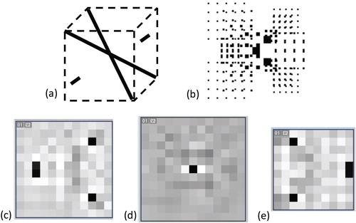
The planes ±3 are taken because the side spots lie at those heights, and the diagonals are not in the corners of the cube. In the output of the wavelet transform in the corresponding depth planes, the cross-sections of the diagonals are clearly recognizable, together with the side spots. Across all the depth planes, the recognized features describe the testing shape exactly.

Compared to the full-parallax case in [36], the recognized points are identified more sharply and thus more accurately.

The next example is an image taken with a plenoptic camera. This image is provided ‘free to use’ at the website of T. Georgiev. This image consists of approx. 100 cells. The recognized objects are as follows (see Figure 13). In the −4th plane, two branches of the tree are recognizable; in plane 0, the wheel and the front of the car are recognizable; and in the 2nd plane, the door and the window of the house are recognizable. The depth of these locations qualitatively corresponds to the layout of the scene.

Figure 13. Wavelet coefficients in the depth planes −4, 0, and +2. Test object ‘house’ (credit to T. Georgiev, www.tgeorgiev.net), available (‘free to use’).

5. Discussions

The model has already been applied to the multiview wavelets [36], to the estimation of the image quality [45,55], to the estimation of the probability of the pseudoscopic effect [31], and to the measurements of the geometric characteristics of displays [35] (i.e. the OVD). The first application relates to the depth planes in the image region; the three others (quality, pseudoscopic effect, and OVD) relate to the fragmentation of the observer region and the layout of the sites. In both cases, the regularity and periodicity of the sites are essential.

The model can also be a useful and flexible tool for many other applications. Among the possible applications are analyzing regions, image cells, and image mixing; designing autostereoscopic displays (full-parallax and HPO displays with rectangular, hexagonal, and slanted image cells); measurement, analysis, simulation, and control of the geometric characteristics of 3D displays [35,56]; and analyzing the depth and resolution [26]. There can be many other applications (e.g. controlling the viewing zones [57], 3D cursors, etc.) in the multiview, integral, plenoptic, and light-field displays.

The main concept of the analytical estimation of the quality is counting mixed-view images. Generally, each site contains its individual set of view images, but there are some common properties in the fragmentation of regions, such as a parameter independent of the lateral displacement. The fragmentation pattern is analyzed in the projective space, and a geometric invariant is found.

The optimal observer distance is one of the most important geometric parameters of a 3D display. It is proposed that the fundamental geometric parameters of the autostereoscopic 3D display devices be measured based on the fragmentation of the observer region and the correspondingly designed test patterns. The following geometric parameters can be measured using a monocular measuring camera and the signed distinction function: the OVD, the width of the sweet spot, and the width of the individual viewing zone. The visual appearance of the special test patterns allows automated measurements. An advantage of the projective form is that the width can be measured at an arbitrary distance to the screen.

Generally speaking, the corresponding cell is not necessarily the closest cell to the current light source.

The screen locations in front of the array of light sources or behind it correspond to the real and virtual modes of integral imaging. Efforts were made, however, not to draw much attention to this, especially because the composite image in the screen plane can be transformed between the two cases (the physical light source and the lens) by means of the inversion of the local coordinates within each cell [43]. Strictly speaking, in the current implementation of the wavelets, the restored location is not a point but is an octahedral volume between the depth lines in the projective space. The accuracy of the depth analysis can be improved, however, by redefining the width of the individual pulses of the packet. The highest depth accuracy (the shortest resolvable distance) will be equal to the double-interline distance in Equation (28) divided by the number of pixels in the cell (note that in the Cartesian space, the result will depend on the distance).

6. Conclusions

An analytical description of multiview images based on the typical structure of autostereoscopic displays is proposed. The main results of this research are the clear analytical description of the space around a 3D display in the projective coordinates. It is based on projections and is therefore periodic and extendable. One application is discussed: the wavelet analysis of multiview images. Based on these results, it may be assumed that the synthesis of 3D images can also be based on these multiview wavelets. In that case, other applications, such as the 3D cursor, will be possible.

Disclosure statement

No potential conflict of interest was reported by the authors.

ORCID

Vladimir Saveljev http://orcid.org/0000-0003-2187-704X

Irina Palchikova http://orcid.org/0000-0002-9039-7157

Correction Statement

This article has been republished with minor changes. These changes do not impact the academic content of the article.

Additional information

Funding

This work was partially (for I. Palchikova) supported by Russian Foundation for Basic Research [grant number 17-47-540269].

Notes on contributors

Vladimir Saveljev

Vladimir Saveljev is a research professor at Myongji University, Yongin, South Korea. He received his M.S. degree from Novosibirsk State University in 1976, and his Ph.D. from the Institute of Automation and Electrometry, Siberian Branch of the Russian Academy of Sciences in 2014. Before occupying his current position, he was with the mentioned institute as well as with Korea Institute of Science and Technology (KIST) and Hanyang University, both in Seoul, South Korea. He is the author of more than 150 research papers and has written 3 book chapters. His current research interests include autostereoscopic 3D displays, image quality, moiré effect, wavelet transform, and nanoparticles.

Irina Palchikova

Irina Palchikova (b. 1954) graduated from Novosibirsk State University (NSU), Russia in 1976, majoring in Physics and Applied Mathematics. She received her Doctor in Physics and Maths degree from NSU in 2000. She is a full professor at NSU, as well as the Head of Laboratory of the Technological Design Institute of Scientific Instrument Engineering SB RAS. Her leading research interests include computer optics, digital image processing, image cytometry, machine vision, and color measurement. She is a member of OSA.

References

- R. Martinez-Cuenca, G. Saavedra, M. Martinez-Corral and B. Javidi, Proc. IEEE 97, 1067 (2009). doi: 10.1109/JPROC.2009.2016816
- B. Lee, S.-G. Park, K. Hong and J. Hong, Design and Implementation of Autostereoscopic Displays (SPIE Press, Bellingham WA, 2016).
- M. Halle, Comp. Graph. 31, 58 (1997). doi: 10.1145/271283.271309
- G. Woodgate and J. Harrold, J. Soc. Inf. Disp. 14, 421 (2006). doi: 10.1889/1.2206104
- A. Kubota, A. Smolic, M. Magnor, M. Tanimoto, T. Chen and C. Zhang, IEEE Signal Proc. 24, 10 (2007).
- N.S. Holliman, N.A. Dodgson, G.E. Favalora and L. Pockett, IEEE T. Broadcast. 57, 362 (2011). doi: 10.1109/TBC.2011.2130930
- C.H. Wu, A. Aggoun, M. McCormic and S.Y. Kung, Proc. SPIE 4660, 135 (2002). doi: 10.1117/12.468026
- J.H. Park, K. Hong and B. Lee, Appl. Opt. 48, H77 (2009). doi: 10.1364/AO.48.000H77
- T. Koike, K. Utsugi and M. Oikawa, in Proceedings of the 3DTV-Conference: The True Vision - Capture, Transmission and Display of 3D Video, edited by A. Gotchev and L. Onural. (IEEE, Tampere, Finland, 2010), pp. 1–4.
- M. Martínez-Corral, A. Dorado, H. Navarro, A. Llavador, G. Saavedra and B. Javidi, Proc. SPIE 9117, 91170H (2014).
- Lytro Support. <https://support.lytro.com/hc/en-us>.
- 3D Light Field Camera. <www.raytrix.de/products/>.
- J.Y. Son, V.V. Saveljev, K.T. Kim, M.C. Park and S.K. Kim, Jpn. J. Appl. Phys. 46, 1057 (2007). doi: 10.1143/JJAP.46.1057
- V. Saveljev and S.J. Shin, J. Opt. Soc. Korea 13, 131 (2009). doi: 10.3807/JOSK.2009.13.1.131
- B.R. Lee, J.J. Hwang and J.Y. Son, Appl. Opt. 51, 5236 (2010). doi: 10.1364/AO.51.005236
- T. Saito, K. Takahashi, M.P. Tehrani and T. Fujii, Proc. SPIE 9391, 939111 (2015). doi: 10.1117/12.2078083
- J.Y. Son, V. Saveljev, S.K. Kim and B. Javidi, Jpn. J. Appl. Phys. 45, 798 (2006). doi: 10.1143/JJAP.45.798
- S.S. Kim, K.H. Sohn, V. Savaljev, E.F. Pen, J.Y. Son and J.H. Chun, Proc. SPIE 4297, 222 (2001). doi: 10.1117/12.430820
- J.Y. Son, V.V. Saveljev, Y.J. Choi and J.E. Bahn, Proc. SPIE 4660, 116 (2002). doi: 10.1117/12.468024
- J. Ren, A. Aggoun and M. McCormick, Proc. SPIE 5006, 65 (2003). doi: 10.1117/12.474128
- J. Bi, D. Zeng, Z. Zhang and Z. Dong, in Proceedings of the World Congress on Computer Science and Information Engineering 6, edited by M. Burgin, M.H. Chowdhury, C.H. Ham, S. Ludwig, W. Su and S. Yenduri (IEEE, Los Angeles, 2009), p. 514.
- J.S. Jang and B. Javidi, Opt. Eng. 44, 01400 (2005).
- D.H. Shin, B. Lee and E.S. Kim, ETRI J. 28, 521 (2006). doi: 10.4218/etrij.06.0206.0014
- S. Manolache, A. Aggoun, M. McCormick and N. Davies, J. Opt. Soc. Am. A 18, 1814 (2001). doi: 10.1364/JOSAA.18.001814
- A. Stern and B. Javidi, Proc. IEEE 94, 591 (2006). doi: 10.1109/JPROC.2006.870696
- J. Hahn, Y. Kim and B. Lee, Appl. Opt. 48, 504 (2009).
- G. Baasantseren, J.-H. Park, N. Kim and K.-C. Kwon, J. Inf. Disp. 10, 1 (2009). doi: 10.1080/15980316.2009.9652071
- R. Ng, M. Levoy, M. Bredif, G. Duval, M. Horowitz and P. Hanrahan, Stanford Tech Report. CTSR 2005-02 (2005).
- T. Georgiev and A. Lumsdaine, J. Electron. Imaging 19, 021106 (2010). doi: 10.1117/1.3442712
- V. Saveljev, J. Inform. Display 11, 21 (2010). doi: 10.1080/15980316.2010.9652123
- V. Saveljev, in Proceedings of the 10th International Meeting on Information Display, edited by S.-D. Lee (SID, K-IDS, Seoul, S. Korea, 2010), pp. 247–248.
- E.F. Pen and V.V. Saveljev, Proc. SPIE 3733, 459 (1999). doi: 10.1117/12.340096
- V.V. Saveljev, J.Y. Son and K.H. Cha, Proc. SPIE 5908, 590807 (2005). doi: 10.1117/12.618167
- V. Saveljev, J.-Y. Son and K.-D. Kwack, in Proceedings of the Spring Conference of Korean Society for Industrial and Applied Mathematics, edited by J.-W. Ra, H.-I. Choi. (KSIAM, Seoul, S. Korea, 2009), pp. 209–212.
- V. Saveljev, in Proceedings of the Winter Annual Meeting of Optical Society of Korea, edited by B.-Y. Kim and G.-W. Ahn. (OSK, Daejeon, S. Korea, 2010), pp. F3F–VIII3.
- V. Saveljev and I. Palchikova, Appl. Opt. 55, 6275 (2016). doi: 10.1364/AO.55.006275
- R. Bregović, P.T. Kovács and A. Gotchev, Opt. Express. 24, 3067 (2016). doi: 10.1364/OE.24.003067
- J.Y. Hong, C.K. Lee, S.G. Park, J. Kim, K.H. Cha, K.H. Kang and B. Lee, Proc. SPIE 9770, 977003 (2016). doi: 10.1117/12.2211823
- V.V. Saveljev, J.Y. Son, S.H Kim., D.S. Kim, M.C. Park and Y.C. Song, J. Disp. Technol. 4, 319 (2008). doi: 10.1109/JDT.2008.922419
- J.Y. Son and B. Javidi, J. Disp. Technol. 1, 125 (2005). doi: 10.1109/JDT.2005.853354
- J.Y. Son, B. Javidi and K.D. Kwack, Proc. IEEE 94, 502 (2006). doi: 10.1109/JPROC.2006.870686
- J.Y. Son, V.V. Saveljev, Y.J. Choi, J.E. Bahn and H.H. Choi, Opt. Eng. 42, 3326 (2003). doi: 10.1117/1.1615259
- Y.S. Hwang, S.H. Hong and B. Javidi, Proc. SPIE 6392, 63920F (2006). doi: 10.1117/12.694541
- J.H. Park, H.R. Kim, Y. Kim, J. Kim, J. Hong, S.D. Lee and B. Lee, Opt. Lett. 29, 2734 (2004). doi: 10.1364/OL.29.002734
- V. Saveljev, J.Y. Son and S.B. Woo, Proc. SPIE. 7329, 73290O (2009). doi: 10.1117/12.821200
- V. Saveljev and S.-K. Kim, in Proceedings of the 17th Conference on Optoelectronics and Optical Communications, edited by B.H. Lee (OSK, Gangwon, S. Korea, 2010), pp. 224–225.
- M. Siegel and L. Lipton, Proc. SPIE 5291, 139 (2004). doi: 10.1117/12.525894
- H.S.M. Coxeter, Projective Geometry (Springer, New York, 2003), Ch. 12.
- A.H. Watt, 3D Computer Graphics (Pearson Education, Harlow, UK, 2000), Chaps. 1, 5.
- V. Saveljev, in Proceedings of the Joint Workshop on the Optical Information Processing and Three-Dimensional Display Technology, Pyeongchang, Gangwon, Korea, edited by S. Lee. (OSK, K-IDS, Pyeongchang, S. Korea, 2009), pp. 101–103.
- V. Saveljev and S.-K. Kim, in Proceedings of the Photonics Conference, Jeju, Korea, edited by K.S. Hyeon. (OSK, Jeju, S. Korea, 2013), pp. 74–75.
- H.S.M. Coxeter, Regular Polytopes (Methuen., London, 1973), pp. 69–72.
- J.Y. Son, V.V. Saveljev, D.S. Kim, S.K. Kim and M.C. Park, Proc. SPIE 6016, 60160N (2005). doi: 10.1117/12.629802
- D. Marr, E. Hildreth, Proc.Roy.Soc. B Biol. Sci. 207, 187 (1980). doi: 10.1098/rspb.1980.0020
- V. Saveljev, J.-Y. Son and K.-D. Kwack, in Proceedings of the International Meeting on Information Display (IMID), edited by H.-D. Park (SID, K-IDS, Seoul, S. Korea, 2009), pp. 1014–1017.
- N.P. Sgouros, S.S. Athineos, M.S. Sangriotis, P.G. Papageorgas and N.G. Theofanous, Opt. Express. 14, 10403 (2006). doi: 10.1364/OE.14.010403
- Y. Hirayama, H. Nagatani, T. Saishu, R. Fukushima and K. Taira, Proc. SPIE 6392, 639209 (2006). doi: 10.1117/12.687075