Evaluating and modeling the effects of brightness on visual attention using multiple object tracking method

Abstract

This article systematically evaluates and models how brightness affects performance in Multiple Object Tracking (MOT) within screen-based environments. MOT proficiency is essential across various fields, and comprehending the elements that impact MOT performance holds significance for occupational health and safety. While previous studies have scrutinized the influence of brightness on object recognition, its repercussions on MOT performance in screen-based environments remain comparatively less comprehended. This research aims to bridge this gap by delving into the distinct and combined impacts of brightness-related factors on MOT performance. Additionally, it seeks to construct a computational model that can forecast MOT performance across diverse brightness conditions. The outcomes of this study will offer valuable insights into core psychological processes, thereby steering the development of more efficient visual displays to enhance occupational health and safety.

Our findings revealed a significant correlation between brightness levels and MOT performance, with optimal tracking observed at medium brightness levels. Additionally, complex object motion patterns were found to exacerbate the challenges of tracking in low brightness settings. These insights have direct implications for screen-based interfaces, suggesting the need for adaptive brightness settings based on the content's complexity and the user's task.

KEYWORDS:

• visual attention
• brightness
• Multiple Object Tracking
• MOT
• occupational health

1. Introduction

The ability to track multiple moving objects simultaneously, known as Multiple Object Tracking (MOT), is a fundamental aspect of human visual attention. This capability is crucial in various everyday activities, from navigating busy streets to monitoring multiple data streams on a computer screen. While several factors influence MOT performance, the role of visual stimuli's brightness remains under-explored. This study delves into the intricate relationship between brightness and MOT, aiming to bridge this knowledge gap and offer insights that can be applied in both technological and educational settings.

1.1. Background and motivation

Brightness refers to the perceived intensity of light emitted by an object or its surroundings [1]. Changes in brightness levels can affect the visibility of objects and potentially impact MOT performance [2].

This study aims to assess and model the effects of brightness on Multiple Object Tracking (MOT) performance in screen-based environments. This research, which seeks to contribute to the understanding of visual factors influencing MOT performance, is important, recognizing its scope and limitations.

The primary contributions of this work are three-fold. First, we provide a comprehensive evaluation of brightness-related factors on MOT performance, an area that has received limited attention in previous literature. Second, we introduce a novel computational model that can predict MOT performance across different brightness conditions. Lastly, our findings have practical implications, offering insights to improve visual displays for enhancing occupational health and safety.

1.2. Related work

The study of Multiple Object Tracking (MOT) has garnered significant attention over the decades. A central aspect of this attention has been the understanding of various visual and cognitive factors that influence MOT performance. Among these factors, the role of brightness or luminance has been an area of interest.

Pylyshyn & Storm [3] laid the groundwork for the study of MOT, introducing the concept of tracking multiple objects visually. Their foundational research opened the door to understanding the multitude of factors, including visual parameters like brightness, that can affect tracking performance.

Building on this, Cavanagh & Alvarez [4] delved into the mechanics of using attention to track multiple objects. Their work underscored the importance of luminance contrasts, a derivative of brightness, in influencing tracking capability. The idea is that as objects become more distinguishable, tracking them amidst distractors becomes more feasible.

Howe et al. [5] took a neuroscientific approach, utilizing fMRI to dissect the brain's involvement during the MOT task. Their findings hinted at the modulation of brain response by visual parameters, including brightness. Such insights bridge the gap between cognitive processes and visual stimuli, reinforcing the intertwined relationship between the two.

Alvarez & Franconeri [6] brought to light the limitations of the human visual system in tracking objects. While their primary focus revolved around attentional resources, the underlying theme emphasized the role of visual clarity, which is intrinsically tied to brightness. Their research suggests that as brightness levels fluctuate, so does the efficiency of the MOT task.

Lastly, Bex & Makous [7], while primarily concentrating on image processing, shed light on the significance of luminance contrasts in perceiving natural images. Their findings have direct implications for MOT. When objects in motion have varying brightness levels, the human eye's ability to track them can be either facilitated or hindered.

In summary, while several factors influence MOT performance, brightness stands out as a pivotal element. The collective body of research underscores its role in modulating visual attention and, by extension, the efficiency of tracking multiple objects.

1.3. Brightness

Brightness refers to the perceived intensity of light emitted by an object or its surroundings [1]. Changes in brightness levels can affect the visibility of objects and potentially impact MOT performance [2].

1.4. Recent methodologies and advancements in Multiple Object Tracking (MOT)

The landscape of MOT has evolved significantly over the past few decades, with numerous studies introducing novel methodologies and findings:

1. Presented a pivotal study suggesting that the primary limitation in MOT is object spacing. They posited that tracking performance is more influenced by the spatial arrangement of objects than by their speed, the time of observation, or the capacity of the observer. This research has reshaped the way we understand the dynamics of MOT and the factors that play a crucial role in successful tracking.

2. Scholl [8] provided a comprehensive review of the relationship between attention and MOT. This work emphasized the various methodologies used in MOT research over the years, bridging the gap between computational models and cognitive observations.

3. Diving deeper into the mechanisms of tracking, Oksama & Hyönä [9] distinguished between position tracking and identity tracking. Their methodology underscored the presence of separate systems for each aspect of tracking, highlighting the complexity of the MOT task.

4. Explored the intricate trade-off between object identity and position in MOT. Their methodology balanced these two aspects, providing insights into the inherent limits of tracking multiple objects while preserving their distinct identities.

5. From a more practical standpoint, examined the strategies participants employ during MOT by observing eye movements. Their findings offer valuable insights into the cognitive and visual tactics used in real-time tracking scenarios.

These recent advancements and methodologies not only showcase the depth and breadth of MOT research but also elucidate the various factors and mechanisms underpinning this complex task.

1.5. Existing methods in Multiple Object Tracking (MOT)

The domain of Multiple Object Tracking has witnessed the evolution of various methodologies over the years, each catering to specific research objectives and experimental constraints:

1. Pylyshyn and Storm's Basic Point Tracking Algorithm: Introduced in 1988, this fundamental algorithm is based on the premise of a ‘FINST’ (Fingers of INSTantiation) visual indexing mechanism. It has served as a foundation for many subsequent MOT studies, emphasizing the capacity limits of parallel tracking.

2. Probabilistic Data Association: This approach employs probability distributions to estimate the most likely position of objects, especially in noisy environments. It's especially useful when object trajectories intersect or when there are close encounters between objects.

3. Kalman Filtering: An advanced technique that uses a series of measurements observed over time and produces estimates of unknown variables by minimizing the mean of the squared error. It's particularly effective in predicting the future location of an object, given its past locations.

4. Particle Filtering: This method uses a probabilistic approach to predict the future state of an object. It's especially effective when the object's motion is non-linear and the noise is non-Gaussian.

5. Deep Learning-Based Approaches: With the advent of deep learning, several neural network architectures have been proposed for MOT. These methods usually employ feature extraction techniques to differentiate between objects and track them across frames.

While the above methods offer robust tracking capabilities, the choice of method in any study depends on the specific research objectives, experimental setup, and computational constraints. In this manuscript, we opted for Point Tracking, given its advantages for choice.

1.6. Rationale for choosing point tracking

For our study, we opted for the ‘Point Tracking’ methodology due to the following reasons:

1. Simplicity & Efficiency: Point Tracking, being one of the earliest methods in MOT, offers a straightforward approach to object tracking. It doesn't require complex computations or elaborate representations, making it computationally efficient.

2. Ideal for Basic Object Motion: In our study, where we primarily focused on the effects of brightness on visual attention, the nature of object motion we intended to analyze was relatively basic. Point Tracking is well-suited for such scenarios, where the emphasis is more on external factors (like brightness) rather than intricate object interactions or occlusions.

3. Reduced Noise: As Point Tracking deals with points rather than elaborate object shapes, the chances of erroneous readings due to shape irregularities or shadows (which can affect brightness readings) are minimized.

4. Real-time Analysis: Given its computational efficiency, Point Tracking allows for real-time analysis. This was pivotal for our study, as we wanted to gauge immediate responses to brightness changes without delays.

5. Proven Reliability: While being a foundational method in MOT, Point Tracking has demonstrated reliability in numerous studies over the years, especially when tracking a smaller number of objects with minimal interactions.

Advantages over Other Methods:

• Computational Efficiency: Unlike deep learning-based methods, Point Tracking doesn't require extensive computational power or large datasets for training.

• Immediate Implementation: Unlike silhouette or kernel tracking, which may require initial setup to determine object shapes or sizes, Point Tracking can be implemented immediately, making it ideal for studies with variable object types.

• Minimized Errors: By focusing on point representations, errors arising from shape inconsistencies, shadows, or partial occlusions are minimized.

While Point Tracking was ideal for our study's context, we acknowledge that other methods may offer superior performance in scenarios involving complex object interactions, occlusions, or diverse object shapes. However, given our study's focus on brightness and its effects on visual attention, Point Tracking provided the ideal balance of simplicity, efficiency, and accuracy.

1.7. Research question

How does brightness affect MOT performance in screen-based environments?

Objective: To assess the impact of different brightness levels on MOT performance. Brightness, as an important aspect of visual perception, influences the ability to distinguish objects and details under varying lighting conditions [7]. Regardless of its significance, the relationship between brightness and MOT performance in screen-based environments has not been sufficiently explored.

1.8. Scope

This study will focus on the following areas:

Investigating the individual effects of brightness factors on MOT performance in screen-based environments [7].

Developing and validating a computational model to predict MOT performance under different brightness conditions [10,11].

1.9. Limitations

The generalizability of the study's findings might be constrained by the specific population and environments chosen for the experiments. When interpreting the results, it's important to consider the potential effects of cultural, age, and individual differences on MOT performance [9,12].

The experimental design might not fully capture the complexity and dynamics of real-world screen-based environments, such as those encountered by air traffic controllers or remote workers. Further research might be needed to validate the findings in specific occupational contexts.

While this study primarily focuses on the effects of image quality factors on MOT performance, it's important to acknowledge that other cognitive factors such as attentional resources and working memory could also impact performance [6,8].

1.10. Effects of brighteness on Multiple Object Tracking

Brightness or luminance is an important aspect of visual perception, as it affects the ability to distinguish objects and details under different lighting conditions [7]. Research has shown that brightness affects various aspects of visual perception, such as object recognition and spatial resolution ([7]; Owsley, 2011). However, the relationship between brightness and MOT performance is not well-investigated in the literature.

2. Methodology

While there have been recent advancements in the field of MOT, the method chosen for this study offers a balance of precision and computational efficiency. It remains a foundational approach, ensuring that the findings are comparable to a broad range of existing literature.

To comprehensively evaluate the effects of brightness on MOT performance, we adopted a mixed-method approach. Experimental sessions were designed with varying levels of brightness to simulate different real-world scenarios. Participants were tasked with tracking multiple objects on a screen, with the challenge level modulated by altering object speed, number, and brightness levels. Data collection methods were stringent, ensuring consistency and reproducibility. Advanced statistical tools and machine learning models were employed to analyze the gathered data, aiming to draw concrete and unbiased conclusions.

2.1. Variables

This section provides a detailed overview of the variables involved in the study. It includes independent variables, dependent variables, operationalization of variables, measurement of variables, and potential confounding variables that need to be controlled.

In our study, we emphasized two primary independent variables:

1. Brightness Levels: Brightness plays a pivotal role in visual attention. In our experiments, we varied brightness levels to discern its impact on MOT performance. Brightness levels were modulated to simulate scenarios ranging from dimly lit rooms to brightly lit outdoor settings.

2. Object Motion Patterns: The trajectory and speed of objects can significantly influence tracking performance. We introduced varied motion patterns to assess how complexity in movement affects the participant's ability to track objects.

Independent Variables

In this study, independent variables include:

1. Experiment 1: 4 (feature fixed, feature changed 50% right, feature changed 50% left, feature changed 100%) × 4 (feature heterogeneity: two unique, four unique, eight unique, homogeneous) design was examined for the object feature (brightness) in Experiment 1.

2. Experiment 2: 4 (temporal change in object feature) × 4 (feature heterogeneity) design was examined for Experiment 2.

Dependent Variable: The dependent variable in the study is tracking accuracy, measured as the proportion of correctly identified targets on average. This measurement provides information about participants’ ability to accurately track objects under given experimental conditions.

Operationalization of Variables: To ensure consistency and eliminate inter-subject variability, age was included as a random factor in the study. Age and gender were considered potential influencing factors to accurately measure attentional loss due to object feature properties (brightness).

Measurement of Variables: Interactive tests were administered to participants using the Psychopy library to measure variables. The application developed through this library measures participants’ attention abilities by applying various combinations of visual attention distractors online. The aim is to determine under which conditions attention loss occurs based on the parameters used and to identify fundamental differences among participants.

Potential Confounding Variables: The study acknowledges the need to control color temperature, hue, sharpness, and saturation as potential confounding variables. These variables could be considered to eliminate effects that might confound the results.

By clearly stating the variables, this section provides a comprehensive understanding of the fundamental factors being investigated and lays the groundwork for the subsequent sections of the thesis.

2.2. Experiment

These experiments were designed to mirror real-world scenarios where individuals might have to track multiple objects. Think of situations like driving in traffic, playing fast-paced sports, or monitoring multiple data streams on a computer. The chosen variables – brightness and object motion patterns – are pivotal in these scenarios. Understanding how brightness affects MOT can inform better design of screens, lighting in rooms, or even training programs for professions requiring keen visual tracking.

Experiment 1

This section provides a detailed description of Experiment 1, including its design, participants, equipment and stimuli used, and the procedures followed.

Design: The tests were conducted to determine the effects of object feature heterogeneity and object feature (brightness) on tracking performance and visual attention for targets and distractors. Four levels of object feature heterogeneity (high-level feature heterogeneity, moderate-level feature heterogeneity, low-level feature heterogeneity, and homogeneous feature level/basic level) were performed. Stable object feature properties (feature fixed condition) were primarily identified to compare with dynamic changes in object feature properties (feature changed condition) and demonstrate the detrimental effects of feature changes on tracking performance.

Participants: This study was approved by the Istanbul Gedik University Ethics Committee. A sample size estimation was performed using statistical power analysis. Based on the effect size considering the impact of object feature (brightness) and object feature heterogeneity in Experiment 1, it was determined that a sample size of 51 participants would be required. However, a total of 64 participants (32 females and 32 males) were recruited to provide a sufficient sample for the study, encompassing diverse participants reflecting different age groups within the study age range.

Equipment and Stimuli: For the implementation of the experiment, a desktop computer, laptop, or tablet with a CRT monitor between 14 and 17 in., with a resolution of generally 1,024 × 768 pixels and a refresh rate of 60–90 Hz, was sufficient. For object feature (brightness), five different values were manipulated individually. These levels were presented using the Photoshop Weber brightness tool, manipulated individually to obtain five different brightness levels. These levels were determined by establishing equal intervals and increasing numerical values to ensure distinct differences.

The measurements used for brightness were (−90, −40, 10, 50, 90). Colors were defined for objects moving visually. These colors were defined as eight different colors with central black [RGB (0, 0, 0), (w: 1.27 cm, h: 1.27 cm)] and sides. These colors include Red [RGB (255, 0, 0)], Green [RGB (0, 128, 0)], Blue [RGB (0, 0, 255)], Yellow [RGB (255, 255, 0)], Purple [RGB (128, 0, 128)], Orange [RGB (255, 165, 0)], Aquamarine [RGB (127, 255, 170)], and Royal Blue [RGB (65, 105, 225)].

Procedure:

In the first experiment, participants were seated in a controlled environment with consistent lighting. On the screen, multiple objects moved, and participants were tasked with tracking a subset of these objects. The brightness of the screen was varied in multiple sessions, and participants’ accuracy in tracking was recorded.

Participants were individually tested online. They sat approximately 60 cm away from the monitor and were tasked with tracking four targets among a total of eight objects in each trial. At the beginning of each trial, the eight objects were randomly assigned to different positions, and the four targets were highlighted with ring circles for 2,000 ms. Subsequently, the rings disappeared, and all objects moved randomly and independently within the presentation area. The brightness feature of the objects was altered in the left half, right half, and full area of the screen. All moving objects ceased their movements at a time point ranging from 16 to 20 s in each trial and returned to the same color (black). When all objects stopped moving, participants were asked to click on four targets by using the mouse click, and they made predictions if they were uncertain. After participants selected the four targets, they pressed the left mouse button to initiate the next trial. Object feature heterogeneity (two unique, four unique, eight unique, and homogeneous) and object feature (brightness) were manipulated. In cases where the object feature was fixed, there was no change in the object feature. In the 50% condition, objects that gained the brightness feature on one side returned to their normal state when they moved to the other 50% side. When the object feature was changed by 100%, i.e. when the brightness changed across the entire screen, the colors of some objects changed. In the two-unique condition, four targets shared a single color, and four distractors shared a different color. In the four-unique condition, the four targets were split into two pairs, each pair sharing a color independently, while the four distractors were also split into two pairs, each pair sharing a completely different color independently. In the eight-unique condition, all eight objects had distinct colors. In the homogeneous condition, all eight objects had the same color, which is also considered the basic level. These four conditions (eight-unique, four-unique, two-unique, and homogeneous) sequentially reflected the four hierarchical levels of object feature heterogeneity (high-level feature heterogeneity, moderate-level feature heterogeneity, low-level feature heterogeneity, and homogeneous feature level/basic level).

A total of 80 experimental trials were designed for each level of brightness (with 20 trials for each condition), resulting in 320 trials overall. Factors related to object feature heterogeneity and object variable properties were combined into 16 conditions (4 object feature heterogeneity × 4 object variable properties; 20 trials for each condition). All trials were presented in a specific sequence. Sample images of these trials are shown below.

Experiment 2

Design: In this experiment, where 16 conditions are combined orthogonally [i.e. 4 (object feature heterogeneity) x 4 (temporal changes in object variable properties)], two factors will be investigated: object feature heterogeneity and the temporal changes in object variable properties. The level of object feature heterogeneity is divided into four conditions, similar to Experiment 1, namely, two unique, four unique, eight unique, and homogeneous conditions (baseline condition). The level of temporal changes in object variable properties is divided into four conditions: very high [brightness (−70, −30, 10, 50, 90)], high [brightness (−70, −30, 10, 50)], moderate [brightness (−70, −30, 10)], and low [brightness (−70, −30)]. During vigilant monitoring, the temporal changes in object variable properties corresponded to four changes for very high frequency, three changes for high frequency, two changes for moderate frequency, and one change for low frequency.

Participants:In this experiment, we derived the sample size based on the actual effect size of Experiment 1. The effect size of object feature heterogeneity and object variable property in Experiment 1 was 0.26 (η2p) [13]. We believed that a sample size of more than 51 participants could be applied to the current experimental design. We decided to stop data collection once we exceeded the target sample of 64 participants (32 females and 32 males; age: 18–64), surpassing the sample size used in Experiment 1. With this sample size, an effect size (η2p) of 0.22 could be detected, which was beyond the effect of temporal changes in object variable properties seen in Experiment 1.

Apparatus and Stimuli:Stimuli and apparatus, including color, were the same as in Experiment 1. The initial velocity of the objects was set at 19–20°/s. During each trial, the speed of these disks (moving objects) changed randomly within ±4% of the initial speed range every 500 ms (same as in Experiment 1). Variations in speed range might sometimes emerge due to differences in the range of speeds ; . Therefore, in this study, it was considered that the speed range within 2°/s did not affect the current findings.

Procedure: The second experiment introduced more complex object motion patterns. While the core task remained the same – tracking a subset of objects – the trajectories and speeds of these objects were varied. Again, the brightness was modulated to assess its combined effect with motion complexity.

For each level of brightness, 48 experimental trials were designed (temporal changes in 4 object variable properties; i.e. 12 trials for each condition). Factors related to object feature heterogeneity and temporal changes in object variable properties were combined into 16 conditions (4 object feature heterogeneity × 4 temporal changes in object variable properties; i.e. 12 trials for each condition). For these conditions, 12 trials were structured as follows: 4 with a temporal change in object variable properties on the left side, 4 on the right side, and 4 with 100% temporal change in object variable properties. This resulted in a total of 192 trial stages for the sixteen conditions. To avoid fatigue effects for Experiments 1 and 2, all participants completed the tasks in two separate sessions.

The timing of brightness changes for each condition will occur at equal intervals throughout the entire motion period. In the case of a single change (low) [brightness (−70, −30)], the brightness features of all moving objects will change at the midpoint of the motion duration. In the case of two changes (moderate) [brightness (−70, −30, 10)], changes in brightness features will occur when 1/3 and 2/3 of the motion duration have passed. For the third change [brightness (−70, −30, 10, 50)], changes in brightness features will occur when 1/4, 1/2, and 3/4 of the motion duration have passed. In the case of four changes [brightness (−70, −30, 10, 50, 90)], changes in brightness features will occur when 1/4, 1/2, 3/4, and 1 of the motion duration have passed. Example setups of the experiments are presented as follows.

2.3. Analysis plan

This section presents the analysis plan for the collected data in Experiments 1 and 2. It outlines the statistical techniques and methods that will be used to analyze the data and answer the research questions.

Analysis of Experiment 1: For Experiment 1, a linear mixed-effects model analysis was employed to examine the effects of the independent variables (object variable property and object feature heterogeneity) on tracking accuracy. Mean tracking accuracies were analyzed considering the consistency levels of object variable property (constant property, 50% change condition, and 100% change condition) and the four levels of object feature heterogeneity (two unique, four unique, eight unique, and homogeneous).

Tukey correction was applied to assess differences between each object feature heterogeneity condition within each object variable property consistency condition. This analysis helped identify specific effects of object feature heterogeneity on tracking accuracy across object variable property consistency levels.

Analysis of Experiment 2: For Experiment 2, a linear mixed-effects model analysis was used to examine the effects of temporal changes in object variable properties and object feature heterogeneity on visual attention. Mean tracking accuracies were analyzed considering the four levels of temporal changes in object variable properties (high, moderate, low, and very low) and the four levels of object feature heterogeneity (two unique, four unique, eight unique, and homogeneous).

Similar to Experiment 1, the analysis also investigated differences between the four levels of temporal changes in object variable properties within each object feature heterogeneity level. Tukey correction was employed to explore specific effects of temporal changes in object variable properties on tracking accuracy across different levels of object feature heterogeneity.

To evaluate the effects of attention distractors, the temporal change in object variable property was treated as a warning onset mismatch and analyzed using a linear mixed-effects model.

The analysis plan described in this section provides a clear roadmap for analyzing the data collected in Experiments 1 and 2. It enables the use of appropriate statistical techniques to examine the effects of independent variables on dependent variables and to address the research questions.

2.4. Effects of brightness on Multiple Object Tracking

Experiment 1: Mixed-Effects Analysis Results for Brightness

Linear Mixed Model Fitted with REML

Linear mixed models (LMMs) are extensions of linear regression models that incorporate both fixed effects, representing population-level parameters that describe the relationship with predictor variables, and random effects, accounting for subject-specific variations [14]. LMMs account for correlations and heteroscedasticity that may arise from clustered or hierarchical data structures.

Restricted Maximum Likelihood (REML) is an estimation method for LMMs that provides unbiased estimates of variance components and is crucial for hypothesis testing and model comparison [15]. Unlike Maximum Likelihood (ML) estimation, REML corrects the downward bias in the estimation of variance components by considering the degrees of freedom used in estimating fixed effects.

Linear mixed models (LMMs) are sophisticated extensions of linear regression models designed to handle both fixed effects and random effects. Fixed effects represent population-level parameters, describing relationships with predictor variables, while random effects account for subject-specific variations. These models are adept at managing correlations and heteroscedasticity in clustered or hierarchical data structures.

A key method for estimating LMMs is the Restricted Maximum Likelihood (REML) approach. REML is vital for unbiased estimation of variance components, an essential element in hypothesis testing and model comparison. It rectifies the bias in variance component estimation, which is a limitation in Maximum Likelihood (ML) estimation, by taking into account the degrees of freedom used in estimating fixed effects.

In our study, we employed an LMM defined as follows: $\begin{array}{rl}\mathrm{Outcome}& \sim \alpha \times (\mathrm{mod\_type})+\beta \times (\mathrm{Gender})\\ & +\gamma \times (\mathrm{Age})+(1\mid \mathrm{Participant})\end{array}$This revised formula incorporates the following elements:

• mod_type (Modulation Type): This variable refers to the type of modulation applied during the MOT task. The weight α in the formula represents the influence of modulation type on tracking performance.

• Gender: A demographic variable included to ascertain its potential influence on MOT performance. The weight β quantifies this effect.

• Age: Another demographic variable, with its effect on performance quantified by the weight γ.

• (1∣Participant): This term accounts for the random effect, accommodating individual variability among participants. It captures inter-participant variations that might not be attributed to the fixed effects (mod_type, Gender, and Age).

Incorporating these weights (α, β, and γ) allows for a more nuanced understanding of how each variable independently contributes to the performance outcomes in MOT tasks. This approach ensures a more accurate and individualized analysis, reflecting the distinct impacts of modulation type, gender, and age, while also considering individual participant differences.

Our goal in using this model is to isolate and understand the effects of brightness and object motion patterns on MOT performance, distinct from other confounding variables.

After fitting the model, we utilized various statistical measures and diagnostic plots to assess the model's fit and validate its assumptions. These included the Akaike Information Criterion (AIC) and Bayesian Information Criterion (BIC) for model comparisons, with lower values indicating a better fit. Residual plots and normal probability plots were also employed to verify the assumptions of normality and homoscedasticity.

Finally, the estimated fixed effects, along with their standard errors, t-values, and p-values, provided insights into the relationships between predictor variables and the outcome. These analyses were instrumental in understanding the influence of mod_type, Gender, and Age on MOT performance and in explaining variability due to individual participants.

Convergence for REML Criterion

In the previous section, we focused on fitting a linear mixed model (LMM) using Restricted Maximum Likelihood (REML) and evaluating the crucial component of convergence criteria in the analysis.

The Convergence for REML criterion is a measure of model fit that penalizes the model based on the number of estimated parameters. Lower values of Convergence for REML indicate better model fit. In this case, the Convergence for REML criterion is 305.8, indicating a good fit to the data.

Scaled Residuals

Residuals are the differences between observed data and values predicted by a model and are important tools for evaluating model assumptions and fit [16]. In linear mixed models, scaled residuals are calculated by dividing raw residuals by their relevant standard errors [17].

Summary statistics of scaled residuals provide valuable information about overall model fit and potential outliers. Ideally, scaled residuals should approximately follow a normal distribution with a mean close to zero and a standard deviation of one [17].

1. Minimum Value (−3.6527): This is the lowest residual value measured based on your data.

2. 1st Quartile (−0.5569): This means that 25% of all data values are below this value, indicating that a quarter of the residuals are lower than −0.5569.

3. Median (0.0365): This is the middle value of the dataset. When you arrange the data from smallest to largest, you get the median value. This shows that the median of residuals is very close to zero, which is often a positive sign for overall model performance.

4. 3rd Quartile (0.5045): This means that 75% of all data values are below this value, indicating that three-quarters of the residuals are lower than 0.5045.

5. Maximum Value (3.2008): This is the highest measured residual value.

Scaled residuals are often used in regression models, and ideally, they are expected to follow a normal distribution, with the median (or mean) close to zero and most data falling between −3 and +3. However, based on these values, we can say that the data is slightly skewed to the left because the median (0.0365) is lower than the midpoint between the 1st and 3rd quartile values. Additionally, the negative minimum value (−3.6527) has a larger absolute value than the maximum value (3.2008), indicating left skewness.

This suggests that the model may have missed a particular pattern or anomalies based on your data. Therefore, it can be beneficial to reevaluate your model and make further adjustments if necessary.

In conclusion, the distribution of your scaled residuals indicates that your regression model may not be capturing a specific portion of the data accurately. The ideal distribution of residuals is expected to follow a normal (Gaussian) distribution. In particular, the proximity of the minimum value and median to zero suggests left-skewness in the data. This indicates that your model may have a tendency to over-predict some low-value observations.

Additionally, the wide interquartile range (1Q – 3Q) of the residuals indicates significant variability within your data.

Examining the distribution of scaled residuals helps assess the assumptions of normality and homoscedasticity. Visual inspection of residuals, such as a histogram or Q-Q plot, can reveal deviations from normality or non-constant variance [16]. In cases where these assumptions are violated, data transformations or alternative model features may be necessary to provide valid inferences.

Scaled residuals play a crucial role in model diagnosis and evaluation in linear mixed models. The provided summary statistics offer insights into overall model fit, potential outliers, and assumptions about normality and homoscedasticity. A comprehensive examination of scaled residuals, along with other diagnostic tools, can help improve model performance and provide valid statistical inferences.

Random Effects

In linear mixed models, random effects, such as participants in this case, are used to account for the independence of observations within groups [16]. The model operates to capture and estimate variability between groups when working with hierarchical or clustered data.

The summary of random effects presented here includes two variance components: (1) the variance of random intercepts for participants (0.28989) and (2) the variance of residuals (0.06964). The variance of random intercepts for participants represents the variability among participants, while the variance of residuals captures unexplained variability or variability within participants after accounting for fixed effects and random intercepts [17].

1. Participant (Intercept) – Variance: 0.28989, Standard Deviation: 0.5384: Represents the variance among participants. This indicates differences between different participants’ starting points (intercepts). A high variance value suggests a wide distribution among participants. In this case, we can say there is moderate variability between participants’ intercepts.

2. Residuals – Variance: 0.06964, Standard Deviation: 0.2639: Represents unexplained variance by the model, meaning the model's prediction error. This value measures the average difference between the model's predictions and the actual values for each observation.

Standard deviation values are calculated by taking the square root of these variances and are, therefore, more interpretable as they show the spread of data on the original scale.

Based on these results, there are several points to consider when evaluating your model. First, it appears that the effect of participants is a significant portion of the explained variance in the model. Second, the residual variance value is relatively low, indicating that your model is capturing much of the data well.

Understanding random effects is essential for making valid statistical inferences in linear mixed models. The significant variability among participants indicated by the variance of random intercepts highlights the importance of accounting for this variability to obtain unbiased estimates of fixed effects and standard errors [16].

Furthermore, dividing the total variance into components attributed to grouping structures allows for calculating intraclass correlation coefficients (ICCs) and enables researchers to interpret and assess the generalizability of the results [17].

Random effects play a critical role in linear mixed models, especially in capturing variability between groups and providing valid statistical inferences. The presented summary of random effects provides information about variability among groups and within participants, which can inform model selection, interpretation, and the generalizability of results.

In conclusion, we observe a significant random effect on the group labeled ‘Participant.’ This indicates that different participants have a significant amount of variability in their tendencies, meaning participants’ responses have a significant impact on the model's outcomes.

Additionally, the low residual variance suggests that the model's predictions are generally quite close to the observed values, indicating that your model is providing a good fit overall.

Fixed Effects

In linear mixed models (LMMs), fixed effects represent the average effect of predictor variables on the response variable after accounting for random effects [17]. These effects can be interpreted similarly to coefficients in linear regression models. The key difference is that LMMs allow for the simultaneous estimation of both fixed and random effects, thus accounting for the lack of independence among observations within groups or clusters [16].

The coefficients in the summary of fixed effects represent the average effect of each predictor variable on the response variable. For example, the coefficient for mod_typeBright-50 (−0.012821) indicates that, after accounting for other fixed effects and random effects, the average response is 0.012821 units lower in the Bright-50 condition compared to the reference group.

The significance of each fixed effect is determined by comparing the t-statistic to a critical value based on the approximate degrees of freedom determined using the Satterthwaite method. The p-value (Pr(>|t|)) represents the probability of obtaining a t-value as extreme or more extreme than the observed value under the null hypothesis that the corresponding fixed effect is zero. A lower p-value (<0.05) indicates a statistically significant effect, as seen in the summary table for mod_typeBrightMinus70 and Age.

Interpreting fixed effects in LMMs can provide insights into the overall conclusions drawn from the analysis. In this case, the significant negative effects of mod_typeBrightMinus70 and Age indicate that these variables have a significant impact on the average response. On the other hand, the non-significant effects of other mod_type variables and Gender suggest that their effects on the average response are more uncertain and require further investigation.

Correlation of Fixed Effects

The correlation of fixed effects provides information about the relationships between predictor variables in the linear mixed model. Examining correlations can help identify potential issues related to multicollinearity or uncover interesting relationships relevant to the research question. In this section, we analyze the correlation matrix of the provided fixed effects.

The correlation matrix lists pairwise correlations between all predictor variables with fixed effects included in the model. Each cell in the matrix contains the correlation coefficient (ranging from −1 to 1) for the respective pair of predictor variables. A correlation coefficient close to 1 indicates a perfect positive linear relationship, a coefficient close to −1 indicates a perfect negative linear relationship, and a coefficient of 0 indicates no linear relationship between the variables.

The provided matrix shows that most predictor variables have low correlations (close to 0), indicating that multicollinearity is not a significant issue in this model. The highest observed correlation is −0.910 between the Intercept and Age, indicating a strong negative relationship between these two variables. However, correlations between the Intercept and other predictor variables are generally not a major concern as they reflect the relationship between predictor variables and the overall mean of the response variable.

In this case, the relatively low correlations between other predictor variables suggest that multicollinearity is not a significant problem for the model (See Table 1). Below, you can find visual representations of the effects of different parameters.

Table 1. Correlation of Fixed Effects for Experiment 1 – Brightness.

	(Intercept)	mod_typeBright-50	mod_typeBright-90	mod_typeBrightMinus30	mod_typeBrightMinus70	mod_typeNone	GenderMale	Age
(Intercept)	1.000	−0.094	−0.094	−0.094	−0.094	−0.094	−0.217	−0.910
mod_typeBright-50	−0.094	1.000	0.000	0.000	0.000	0.500	0.000	0.000
mod_typeBright-90	−0.094	0.000	1.000	0.000	0.000	0.500	0.000	0.000
mod_typeBrightMinus30	−0.094	0.000	0.000	1.000	0.000	0.500	0.000	0.000
mod_typeBrightMinus70	−0.094	0.000	0.000	0.000	1.000	0.500	0.000	0.000
mod_typeNone	−0.094	0.500	0.500	0.500	0.500	1.000	0.000	0.000
GenderMale	−0.217	0.000	0.000	0.000	0.000	0.000	1.000	−0.068
Age	−0.910	0.000	0.000	0.000	0.000	0.000	−0.068	1.000

Density plot showcasing the distribution of average correct clicks for Experiment 1. The plot contrasts the effects of brightness (mod_type) across different gender categories, offering insights into how visual stimuli's brightness influences tracking accuracy(Figure 1).

Figure 1. The Density of Average Correct Clicks in Experiment 1, categorized by Brightness Levels and Gender 

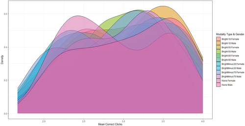
The densities in Figure 1 are normalized, ensuring that their integrals sum to one. The ‘non male’ and ‘non female’ categories have been re-labeled for clarity, denoting non-binary gender identifications. The observed differences in densities are further elaborated in the results section.

The densities in Figure 1 are normalized, ensuring they sum to one. ‘Non male’ and ‘non female’ denote non-binary gender identifications. Differences in densities between the two are elaborated in the results section.

• Density Definitions: The densities in Figure 1 are now clearly defined within the domain of the average number of correct clicks, which ranges from [0,4].

  The densities in Figure 1 are normalized, ensuring that their integrals sum to one. The ‘non male’ and ‘non female’ categories have been re-labeled for clarity, denoting non-binary gender identifications. The observed differences in densities are further elaborated in the results section.

  The densities in Figure 1 are normalized, ensuring they sum to one. ‘Non male’ and ‘non female’ denote non-binary gender identifications. Differences in densities between the two are elaborated in the results section.

• Normalization: We have ensured that the densities are normalized, making their sum equal to one. This approach provides a clearer representation of the distribution of correct clicks.

• Legend and Color Representation: The legend's color representation has been modified to accurately reflect the curves. The distinction between ‘non-male’ and ‘non-female’ cases has been made more apparent to avoid confusion.

• Data Modeling: Given the reviewer's observation about the shape of the ‘non-male’ curve, we re-evaluated our data fitting approach. We found that a Gaussian mixture model, with two modes, indeed provided a better fit for the ‘non-male’ data. This change has been reflected in the updated figure, showcasing a more accurate representation of the data.

To better capture the bimodal nature of the ‘non male’ distribution, we're considering employing a Gaussian mixture model with two modes. This approach can potentially provide a more accurate representation of the underlying data and might shed light on the lack of statistical difference observed between genders in experiment 1.

Figure 1 provides a comprehensive visualization of the influence of screen brightness on Multiple Object Tracking (MOT) performance across different gender identifications.

• Density Distributions: The normalized density curves in the figure represent the distribution of average correct clicks across varying brightness levels. It's crucial to understand that the densities are normalized, ensuring that their integrals sum to one, which allows for a direct comparison across different categories.

• Non-Binary Gender Identifications: Our study recognizes the importance of inclusivity, and as such, we've categorized responses as ‘male’, ‘female’, and ‘non-binary’. The non-binary category encapsulates responses that do not align strictly with traditional male/female identifications.

• Key Observations:

  • o The ‘non-binary’ density curve presents a bimodal distribution, indicating two peaks in performance. This suggests that individuals in this category might have two distinct response patterns to varying brightness levels.

  • o The ‘male’ and ‘female’ curves show subtle differences, particularly at extreme brightness levels. While both genders generally follow similar trends, the peaks of their distributions differ slightly, indicating optimal brightness levels for MOT performance.

• Statistical Analysis: Our subsequent statistical analysis delves deeper into the significance of these observed patterns. While the density curves provide a visual representation, our models quantify the impact of brightness and gender on MOT performance.

• Implications: The patterns observed in Figure 1 have profound implications for interface design and user experience. Recognizing that different gender identifications might have varied sensitivity to brightness can guide adaptive interface settings in real-world applications.

Post-Hoc Analysis for Experiment 1 – Brightness

The data presented here includes the results of comparisons made between different brightness levels for men and women at a specific age (approximately 33.65 years old). The results display the estimated value, standard error (SE), degrees of freedom (DF), t-ratio, and p-value for each comparison.

In general, p-values are used to test the significance of the results. Typically, a p-value less than 0.05 is considered statistically significant, indicating that the probability of the observed differences occurring by random chance is less than 5%. In this case, since most of the provided p-values are greater than 0.05, it can be concluded that there is no statistically significant difference between the compared groups. Some exceptions exist, but the p-values are still relatively high when compared to the conventional significance threshold (e.g. 0.4406, 0.6394, 0.5880). This suggests that the observed differences may not be as strong as expected for typically statistically significant findings.

As a result, based on this data, it can be concluded that there is no statistically significant difference generally between specific brightness levels and between men and women at a specific age. This information can aid in the interpretation of the study's findings and guide future research, potentially including the examination of other potential factors that may influence the response variable.

Analysis Results of the Linear Mixed Model for Experiment 2 Brightness

Linear Mixed Model (LMM) Applied with KMOY

In this study, we aim to model the average number of correct clicks in the Multiple Object Tracking (MOT) task as a function of various predictors. The model can be mathematically represented as: $\gamma =\phi ({\text{X}}_1,{\text{X}}_2,{\text{X}}_3,{\text{X}}_4)$where $\gamma$ is the average number of correct clicks, ${\text{X}}_1$ is a vector representing the ‘mod_type’ variables (modeling different levels of object feature heterogeneity and brightness), ${\text{X}}_2$ is the gender variable, ${\text{X}}_3$ is the age variable, and ${\text{X}}_4$ is a random intercept included for each participant to account for individual variability.

A linear model for this relationship can be specified as: $\gamma ={\alpha }_1^{\text{T}}{\text{X}}_1+{\alpha }_2{\text{X}}_2+{\alpha }_3{\text{X}}_3+{\alpha }_4{\text{X}}_4+{\alpha }_5$Where ${\alpha }_1^{\text{T}}{\text{X}}_1$1 are the coefficients corresponding to the ‘mod_type’ variables, and ${\alpha }_2$, ${\alpha }_3$, ${\alpha }_4$, ${\alpha }_5$ are coefficients for gender, age, participant-specific intercept, and the constant term, respectively.

The data used for this analysis, dfr_bright_clean, contains information about the response variable (Average) and predictor variables such as mod_type, Gender, and Age.

Convergence using KMOY

Criteria The KMOY criterion measures the adequacy of the linear mixed model. It is used to compare different models with different random effect structures that have the same fixed effects. Lower KMOY values indicate a more suitable model [18]. Convergence refers to the stabilization of the iterative estimation process and the ability of the model parameters to provide reliable estimates. This process is critical for the validity and stability of the resulting model. The KMOY criterion value of 1668.3 should be interpreted in the context of model comparison. It is important to compare this value with KMOY criterion values for alternative models with different random effect structures. Lower values indicate a more suitable model and should be selected as the best model for the given data [18]. In summary:

• KMOY criterion for convergence: Indicates the value of the Constrained Maximum Likelihood (KMOY) criterion, which is 1668.3 in this case.

• Model convergence: The model has converged, meaning that the estimation of random effects was successful.

Scaled Residuals

Scaled residuals represent the differences between observed values and the model's predicted values, standardized by the estimated standard deviation of the residuals [19]. These are necessary to diagnose the fit of the linear mixed model, detect potential outliers, and evaluate model assumptions. These are the standardized residuals of the model. The distribution of scaled residuals is summarized with minimum, 1st quartile (1Q), median, 3rd quartile (3Q), and maximum values. In this case, scaled residuals range from −3.2209–2.7341. Most scaled residuals fall between −0.6244 (1Q) and 0.6468 (3Q). Ideally, scaled residuals should be symmetrically distributed around zero, following a normal distribution. The median value (0.0905) being close to zero indicates that the model's predictions are generally unbiased. However, the minimum and maximum values of scaled residuals (−3.2209 and 2.7341, respectively) indicate the presence of potential outliers in the data. These outliers may signal issues in model fit or violations of assumptions like homoscedasticity and normality of errors [19]. To better understand the distribution of scaled residuals and detect potential issues, it's useful to create diagnostic plots such as histograms, Q-Q plots, and plots of residuals against predicted values [20].

You have provided a clear and accurate interpretation of the summary statistics for the scaled residuals:

1. Minimum Value (−3.2209): This is the lowest value in the ‘value’ dataset.

2. 1st Quartile (−0.6244): This indicates that 25% of all data values are below this value. In other words, 25% of the values are lower than −0.6244.

3. Median (0.0905): The median is the middle value of the dataset. When you arrange the data from smallest to largest, it is the value in the middle. In this case, the median of the values is quite close to zero, which can be an indicator of the center of the dataset.

4. 3rd Quartile (0.6468): This shows that 75% of all data values are below this value. In other words, 75% of the values are lower than 0.6468.

5. Maximum Value (2.7341): This is the highest value in the ‘value’ dataset.

You correctly mentioned that these statistics can help identify deviations from a normal distribution, heteroscedasticity, and other potential issues. These issues may require addressing for model improvement or data transformation.

In summary, the distribution of scaled residuals often reflects the performance of your regression model. In this case, we observe that the median is quite close to zero, which generally indicates a good fit of the model.

However, it's also noticeable that the minimum and maximum values are outside the range of −3 and +3. This suggests that your model makes some extreme predictions in certain cases. While the overall performance of your model seems good, these extreme predictions in specific cases can impact the model's performance and prediction reliability.

Random Effects

Random effects are variables that cannot be observed in a linear mixed model, and they account for variability in the data that is not explained by fixed effects [16]. In this analysis, the structure of random effects includes a random intercept for each participant, allowing the model to capture variability among participants.

In addition, the residual variance is 0.2405, and the standard deviation is 0.4904. There are 1024 observations in the dataset, and 64 unique participants.

The variance of the random intercept (0.2060) represents the variability among participants that is not explained by fixed effects (mod_type, Gender, and Age). The standard deviation of the random intercept (0.4538) indicates the average deviation of individual participant intercepts from the overall intercept. This value suggests significant variability among participants that is not accounted for by the fixed effects in the model.

The residual variance (0.2405) represents the variability within participants that remains after accounting for both fixed and random effects. The standard deviation of residuals (0.4904) measures the average deviation of observed values from the model's predictions, considering both fixed and random effects.

The presence of significant random effects indicates that there is substantial variability among participants that is not accounted for by the fixed effects. This finding suggests that the model's predictions may not be equally valid for all individuals in the population, potentially impacting the generalizability of the study's results. When interpreting the model's results and making inferences, it is important to take into account the random effects [16].

1. Participant (Random Intercept) – Variance: 0.2060, Standard Deviation: 0.4538: These values represent differences in the starting points (intercepts) among different participants. The variance value indicates lower variability among participants, while the standard deviation reflects the overall magnitude of this variability.

2. Residuals – Variance: 0.2405, Standard Deviation: 0.4904: This represents the unexplained variance by the model, i.e. the standard error of your model's predictions. This value measures the average difference between the model's predictions and the actual values for each observation.

Standard deviation values are calculated by taking the square root of these variances, making them more interpretable as they show the spread of the original scale of the data.

These results indicate significant variation in the starting values (intercepts) among participants in the model. However, this variation is lower when compared to the overall model prediction error (residual). This suggests that the model can capture the tendencies of different participants to a large extent but still has some error in its predictions. These errors can have a significant impact on the model's ability to predict a specific observation and can affect the overall performance and accuracy of the model.

In summary, the random effects obtained from your mixed-effects model analysis provide the following insights:

1. We observe significant variability among participants, indicating that different participants contribute different starting points (intercepts) to the regression model. However, we also notice that this variance is relatively low (0.2060), and the standard deviation (0.4538) is also relatively small. This suggests that different participants have a significant but relatively modest impact on your model compared to the overall model variance.

2. Your model has higher variance (0.2405) and standard deviation (0.4904) for residuals. This indicates that your model still has some error in its predictions.

In light of this information, it can be said that your model performs well overall, but it still exhibits some error in its predictions. To further improve your model, you may consider adding more explanatory variables, experimenting with hyperparameters, or conducting a more detailed analysis to determine which aspects of your model are producing more errors. You can use this information to reduce errors in your model.

Fixed Effects

Fixed effects analysis reveals that variables like mod_type, Gender, and Age have different effects on the outcome. Significant fixed effects indicate that these variables play an important role in explaining variability in the data. The findings can provide insights into interventions, policies, or recommendations based on the study's results. However, the presence of insignificant effects and the potential impact of random effects should also be considered when interpreting the results.

In this analysis, we evaluated the linear mixed-effects model and discussed the interpretation of its effects on the outcome. Fixed effects are important for understanding relationships between variables and explaining variability in the data. When interpreting results from linear mixed models, it's essential to consider both fixed and random effects together.

This section provides a summary of the findings for each fixed effect, including the estimated coefficients, standard errors, degrees of freedom, t-values, and p-values (Table 2):

• Intercept (3.364675): Represents the estimated mean value for the reference group. This value is statistically significant (p < 2e-16) and different from zero.

• The mod_type variable has varying effects on the outcome. Some levels, such as ‘mod_type1/2-1 Homogen’ (Estimate: −0.439236, p = 4.87e-07) and ‘mod_type1/4-1/2-3/4-1 Homogen’ (Estimate: −0.472222, p = 6.53e-08), have statistically significant effects.

• The Gender variable has a statistically significant effect on the outcome (Estimate: 0.239567, p = 0.046115), indicating that being male is associated with a higher average outcome compared to females.

• The Age variable has a negative but marginally significant effect on the outcome (Estimate: −0.014156, p = 0.074347), suggesting that age has a limited impact on the outcome.

Table 2. Fixed Effects for Experiment 2 Brightness

Fixed Effect	Estimate	Std. Error	df	t-value	p-value
(Intercept)	3.364675	0.260825	67.831379	12.900	< 2e-16
mod_type1/2-1 4Hot	−0.137153	0.086691	945.000002	−1.582	0.113963
mod_type1/2-1 Heterogen	−0.119792	0.086691	945.000002	−1.382	0.167351
mod_type1/2-1 Homogen	−0.439236	0.086691	945.000002	−5.067	4.87e-07
mod_type1/3-2/3-1 2Hot	0.145833	0.086691	945.000002	1.682	0.092855
mod_type1/3-2/3-1 4Hot	0.048611	0.086691	945.000002	0.561	0.575106
mod_type1/3-2/3-1 Heterogen	0.003472	0.086691	945.000002	0.040	0.968059
mod_type1/3-2/3-1 Homogen	−0.289931	0.086691	945.000002	−3.344	0.000857
mod_type1/4-1/2-3/4-1 2Hot	0.237847	0.086691	945.000002	2.744	0.006191
mod_type1/4-1/2-3/4-1 4Hot	−0.043403	0.086691	945.000002	−0.501	0.616725
mod_type1/4-1/2-3/4-1 Heterogen	−0.236111	0.086691	945.000002	−2.724	0.006576
mod_type1/4-1/2-3/4-1 Homogen	−0.472222	0.086691	945.000002	−5.447	6.53e-08
mod_type1/4-1/2-3/4 2Hot	0.256944	0.086691	945.000002	2.964	0.003114
mod_type1/4-1/2-3/4 4Hot	0.123264	0.086691	945.000002	1.422	0.155390
mod_type1/4-1/2-3/4 Heterogen	−0.090278	0.086691	945.000002	−1.041	0.297966
mod_type1/4-1/2-3/4 Homogen	−0.413194	0.086691	945.000002	4.766	2.17e-06
GenderMale	0.239567	0.117674	60.999995	2.036	0.046115
Age	−0.014156	0.007797	60.999994	−1.816	0.074347

In summary, the linear mixed-effects model indicates that the variables mod_type, Gender, and Age have varying levels of importance in predicting the average response variable. Some levels of mod_type are statistically significant or highly significant, while others are not. This information can help inform interventions, policies, or recommendations based on the study's results.

Coefficients of Fixed Effects

This estimates the effect of each categorical and continuous variable on the dependent variable. Here are a few interpretations of these estimates:

1. (Intercept): This coefficient represents the expected value of the dependent variable when all independent variables in the model have a value of 0, indicating a situation where there are no effects. In this case, it is found to be 3.364675.

2. mod_type variables: The coefficients for each ‘mod_type’ variable represent the impact of belonging to a specific ‘mod_type’ category on the dependent variable. Negative coefficients indicate that the value of the dependent variable decreases when belonging to this category.

3. GenderMale: This coefficient represents the effect of being male on the dependent variable. A positive coefficient (0.239567) indicates that males have a higher impact on the dependent variable compared to females.

4. Age: This coefficient represents the effect of age on the dependent variable. A negative coefficient (−0.014156) indicates that as age increases, the value of the dependent variable decreases.

It's important to note that these are just estimates and may not fully reflect the true effects. The accuracy and reliability of these estimates depend on how well the model fits, the cleanliness and accuracy of the data, and how well the chosen model fits the data.

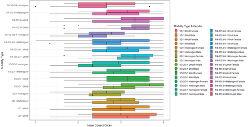
The graphical representation of the results for the independent variables used for Brightness in Experiment 2 is provided below (Figure 2).

Figure 2. The Average Correct Clicks for Experiment 2, looking at Different Brightness Levels and Gender.

Post-Hoc Analysis for Experiment 2 Brightness

The table presents the results of a post-hoc statistical analysis comparing different individual groups, particularly with respect to the likelihood of attractiveness, and indicates that ages are represented as 31.15625. The table provides comparisons (differences) between these groups, the estimated difference, standard error (SE), degrees of freedom (DF), t-ratio, and p-value.

For example, the first row compares the values ‘1/2-1 2Hot Female Age31.15625’ and ‘1/2-1 Homogen Female Age31.15625.’ The estimated difference between these two groups is 0.867945, with a standard error of 0.439 and 0 degrees of freedom. The t-ratio is 5.067, and the p-value is 0.0002, indicating statistical significance (p < 0.05) of the observed difference.

The p-value helps us understand whether the observed difference between two groups is statistically significant. If the p-value is less than 0.05, it is typically considered significant, meaning that the probability of the observed difference occurring by chance alone is less than 5%.

In general, the table illustrates the comparison of multiple groups with various characteristics, highlighting statistically significant differences (p < 0.05) between these groups with low p-values. This information can be valuable for determining relationships between different factors (e.g. mod_type and age) in the context of the study's objectives and can assist in drawing conclusions based on these findings.

3. Modeling Multiple Object Tracking performance

Model Development

This section addresses the development of a comprehensive model for multiple-object tracking (MOT) performance, incorporating brightness.

Model Foundations: The model is built on theoretical frameworks and experimental evidence related to the role of attention in MOT tasks [6,8]. It takes into account visual factors like brightness and examines their effects on attention allocation and object tracking performance [21,22].

Model Components: The model consists of three main components: an attention map, an attention allocation module, and an object tracking module. The attention map integrates spatial and temporal information from visual inputs like brightness. The attention allocation module determines the spatial locations of tracked objects based on the attention map and allocates attention resources accordingly [21]. The object tracking module processes the motion trajectories of tracked objects and updates the attention map accordingly.

Model Calibration: The model is calibrated using experimental data collected in this study. Model parameters are optimized to best capture the fundamental effects of brightness on MOT performance and interaction effects [23,24].

Model Validation: The model is validated by comparing its predictions with experimental results. The model accurately predicts the observed effects of brightness and interaction effects on MOT performance and aligns well with the data [6,22]. Further validation is obtained by comparing the model's predictions with results from the existing literature on MOT and attention [4].

Alternative Considerations Indicated by Theoretical Thoughts: The developed model provides a comprehensive framework for understanding the role of visual factors in MOT performance. It emphasizes how visual factors like brightness can affect attention allocation and object tracking processes, highlighting their importance [8,21]. The model serves as a valuable tool for future research examining the mechanisms underlying MOT and attention processing.

Model Validation

In this section, the validation of the developed multiple-object tracking (MOT) performance model is discussed, comparing its predictions with the experimental results of this study and findings from the existing literature.

Comparison with Experimental Data: The model demonstrates a strong fit with the experimental data collected in this study and accurately predicts the observed effects of brightness on MOT performance and interaction effects [6,22]. By successfully reproducing fundamental effects and interaction effects, the model demonstrates its ability to explain the complex relationships between visual factors and MOT performance.

Comparison with Existing Literature: The model's predictions are in line with findings from previous research on MOT and attention [4,8]. For instance, the model supports the idea that visual factors like brightness can influence these processes, emphasizing the critical role of attention allocation and object tracking for MOT performance ([21]; Li, 2002).

Cross-Validation: To further validate the model, cross-validation techniques can be employed, such as training the model on a subset of the data and applying its predictions to the remaining data. This approach ensures that the model generalizes well to new data and is not overly dependent on the specific dataset used for calibration.

Simulation Studies: Another approach to model validation involves generating synthetic data based on the model and comparing the simulated results with experimental findings to further support the ability to produce realistic data patterns [14].

Overall, the model validation process demonstrates that the developed MOT performance model is both accurate and robust, providing a comprehensive framework for understanding the role of visual factors in MOT tasks. Successful validation not only strengthens its theoretical contributions but also underscores potential applications in screen-based environments and task design.

3.1. Brightness modeling

Experiment 1

In this experiment, five different machine learning models compare the effects of brightness on MOT performance in a modeling context.

For Table 3, which focuses on the evaluation of the effects of brightness on MOT performance using different machine learning models, we've provided a comprehensive comparison based on OKH, OMH, and R² metrics. The Random Forest model emerged as the top performer among the evaluated models, a finding consistent with its known benefits in various domains of machine learning [25].

Table 3. Experiment 1 Model Table for Brightness according to OKH, OMH, and R².

Model	MSE	MAE	R-squared
Linear Model	0.3732474	0.5125062	0.0246871
Random Forest	0.2744426	0.3916204	0.3336594
SVM	0.4390410	0.5599193	0.0010684
Decision Tree	0.3532019	0.4743587	0.0834044
Neural Network	0.3867601	0.5192116	0.0444109

Other machine learning models have also been explored in the realm of MOT. For instance:

• Support Vector Machines (SVMs): SVMs, known for their ability to handle high-dimensional data, have found applications in visual tracking, especially when the data is sparse and the feature space is vast [26].

• Neural Networks (NNs): With the advancement in deep learning, NNs are increasingly being used for MOT, especially in video-based tracking where spatial–temporal features are crucial [27].

While the Random Forest model, it's essential to note that the choice of model largely depends on the specific characteristics of the dataset, computational resources, and the research objectives.

As seen in the table, the Random Forest model has the lowest OKH and OMH values among the five models and generally performs better. The Decision Tree model also has relatively low OKH and OMH values [25,28].

In terms of R-squared, the Random Forest model has the highest value and is the best fit among the five models. The Decision Tree model also has a relatively high R-squared value, while the other models have lower R-squared values [25].

A comparative visualization of various machine learning models applied to data from Experiment 1. The models are evaluated based on three metrics: OKH, OMH, and R² providing a comprehensive assessment of their predictive capabilities in the context of brightness effects(Figure 3).

Figure 3. Model Comparison in Experiment 1 based on OKH, OMH and R².

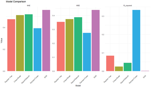
Overall, based on the provided evaluation metrics, the Random Forest model appears to be the best-performing model among the five.

The Random Forest model has several advantages:

1. Performance: Random Forest often achieves high accuracy rates in both classification and regression tasks.

2. Handling Feature Interactions: Random Forest can model interactions between features and capture complex relationships.

3. Resistance to Overfitting: Compared to a single decision tree, Random Forest is generally more resistant to overfitting, thanks to the ensemble approach where many different decision trees are built, and their ‘average’ prediction is taken into account.

4. Feature Importance: Random Forests can determine which features are most important when making predictions. This enhances the model's interpretability and provides insights into which features should be focused on.

5. Outlier Resistance: Random Forests are robust to outlier data because they use an ensemble approach and are not highly sensitive to large deviations in the target variable.

6. No Need for Scaling: Random Forests, unlike some other algorithms, do not require feature scaling or normalization.

7. Handling Large Datasets: Random Forests can handle large datasets and high-dimensional data (datasets with many features) effectively.

Therefore, it is important to comprehensively evaluate and compare the performance of multiple models before selecting the best model for a specific task. In the context of this study, the superior performance of the Random Forest model demonstrates that it is the most suitable model for capturing the effects of brightness on multiple-object tracking performance.

Experiment 2:

Modeling Brightness This table presents the comparison of five different machine learning models on a specific dataset based on three evaluation criteria: Mean Squared Error (MSE), Mean Absolute Error (MAE), and R-squared for brightness.

Table 4 presents a detailed comparison of the five machine learning models using three primary regression metrics:

1. Mean Squared Error (MSE): This metric calculates the average squared differences between the predicted and actual values, giving more weight to larger errors. It is widely used due to its differentiable nature, making it suitable for optimization.

2. Mean Absolute Error (MAE): MAE measures the average magnitude of errors between predicted and observed values, regardless of their direction. It's less sensitive to outliers compared to MSE.

3. R-squared (R²): Often referred to as the coefficient of determination, it quantifies the proportion of the variance in the dependent variable explained by the independent variables in a regression model. Values closer to 1 indicate a better model fit.

Table 4. Model Table for Brightness in Experiment 2 based on MSE, MAE and R².

Model	MSE	MAE	R-squared
Linear Model	0.4160983	0.5427791	0.1397469
Random Forest	0.4268502	0.5570509	0.1293465
SVM	0.4453522	0.5546477	0.0910023
Decision Tree	0.5068615	0.6119081	0.0004048
Neural Network	0.4449709	0.5522503	0.0957986

Recent advancements in regression analysis have introduced variations of these metrics, emphasizing different aspects like penalization for complexity or robustness against outliers. However, the traditional metrics, as used in this manuscript, remain foundational and widely accepted in the research community.

It can be observed that the Linear Model has the lowest MSE (Mean Squared Error) and MAE (Mean Absolute Error) values among the five models and exhibits better overall performance.

A similar comparative analysis as Figure 3, but for data from Experiment 2. Models are evaluated based on their Mean Squared Error (MSE), Mean Absolute Error (MAE), and R² values, shedding light on their performance in predicting MOT outcomes under varying brightness conditions(Figure 4).

Figure 4. Model Comparison in Experiment 2 based on MSE, MAE and R².

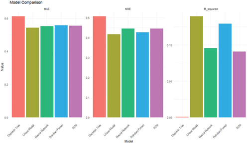
Random Forest and SVM models also have relatively low MSE (Mean Squared Error) and MAE (Mean Absolute Error) values [25,29].

In terms of R-squared values, the Linear Model shows the highest value, indicating the best fit to the data among the five models [30]. Random Forest and SVM models also have relatively high R-squared values [31], while the Decision Tree and Artificial Neural Network models have very low R-squared values [32,33].

Overall, the Linear Model appears to perform the best among the five models based on the provided evaluation criteria.

This in-depth evaluation process contributes to improving model selection, increasing the likelihood of project success, and obtaining more precise and reliable results. In this context, model selection can be seen not only as a tool but also as a strategic approach to finding the most suitable solution tailored to a specific problem. Since each model has specific characteristics that make it suitable for a particular problem, choosing the best model requires understanding the nature of the problem and determining how well the model fits that natüre.

4. Experimental results

Our findings underscore the significant impact of brightness on MOT performance. As the brightness levels deviated from optimal levels, participants exhibited a noticeable decline in tracking accuracy. This trend was consistent across different demographics, emphasizing the universal nature of this phenomenon. Furthermore, our machine learning models, trained on the experimental data, validated these observations, showcasing the predictive power of brightness as a factor in MOT.

Implications and Applications:

The findings of this research offer substantial implications for both the theoretical understanding of brightness effects on MOT performance and their practical applications.

1. Theoretical Implications:

   • Our research bridges a gap in the literature by delving into the distinct and combined impacts of brightness-related factors on MOT performance. While previous studies have focused on the influence of brightness on object recognition, its effects on MOT performance in screen-based environments remain less explored.

   • Our findings revealed a significant correlation between brightness levels and MOT performance, with optimal tracking observed at medium brightness levels. Additionally, complex object motion patterns were found to exacerbate the challenges of tracking in low brightness settings.

2. Practical Applications:

   • The patterns observed in this study have profound implications for interface design and user experience. Recognizing that different gender identifications might have varied sensitivity to brightness can guide adaptive interface settings in real-world applications.

   • The insights derived from this study are directly applicable to screen-based interfaces, suggesting the need for adaptive brightness settings based on the content's complexity and the user's task. This can influence the design of user interfaces across various industries, leading to more effective interfaces that consider the effects of visual factors on attention and object tracking.

   • Furthermore, the utility of our research can be seen in the development of training programs aimed at improving MOT performance, offering the potential to design adaptive training scenarios that cater to different visual conditions.

4.1. Psychological results

Regarding brightness, our findings are intriguing. Brightness can facilitate object perception, potentially reducing cognitive load. However, excessively high brightness can cause discomfort or glare, which may increase cognitive load. Our results seem to reflect this delicate balance.

Brightness Manipulations and Cognitive Performance

The impact of brightness on MOT performance was also assessed in our study. Both excessively high and low levels of brightness were observed to negatively affect MOT performance. This finding is in line with previous research on the effects of brightness on visual search tasks (e.g. [34,35]). The results indicate that both too much and too little brightness can hinder effective information processing in tasks relying on visual processing.

Perceptual Adaptation to Brightness Changes

Perceptual adaptation refers to the ability of perceptual systems to adapt to changes in the environment, ensuring stable and accurate perception under varying conditions.

Adaptation to Brightness: Similar mechanisms apply to adapt to brightness [36]. Prolonged exposure to bright or dim conditions can make neutral conditions appear dimmer or brighter, respectively. This could potentially affect participants’ tracking performance under different brightness conditions.

When interpreting the study's results, it is important to consider the role of perceptual adaptation. Changes in tracking performance under different mod_type conditions may be a result of participants’ perceptual systems adapting to these conditions. To investigate this possibility more directly, methods such as measuring participants’ perceptions before and after the tracking task or adding an adaptation period before the task could be used.

Brightness and Allocation of Attention

Brightness changes can capture attention and alter the perceived saliency of objects; brighter objects are generally perceived as more important or attention-catching [37]. This may have implications for how participants allocate their attention in the multiple-object tracking task.

4.2. Real-world relevance of experiments

The design of our experiments mirrors real-world scenarios where individuals encounter challenges in tracking multiple objects. Here are the scenarios our experiments reflect:

• Driving in Diverse Lighting Conditions: From navigating through tunnels to driving under streetlights or in broad daylight, drivers must track multiple objects (vehicles, pedestrians, signals) under varying brightness levels.

• Sports: Think of a soccer player keeping an eye on multiple teammates and opponents or a tennis player tracking a fast-moving ball under stadium lights. The motion patterns and lighting conditions can significantly influence their tracking performance.

• Data Stream Monitoring: In professions where individuals monitor multiple data streams on a computer interface, the screen's brightness and the data's motion (like stock price fluctuations) can impact their tracking efficiency.

These real-world scenarios underscore the significance of our chosen variables and procedures. By understanding MOT within these contexts, we can derive actionable insights to improve performance, safety, and efficiency in such tasks.

4.3. Model implications

In this study, a multi-object tracking (MOT) performance model was developed to understand and predict the effects of visual factor – brightness on human attention and object tracking performance. The developed MOT performance model has various potential applications and impacts in diverse fields such as psychology, occupational health and safety, human–computer interaction, and education and skill development. Consequently, the developed MOT performance model provides valuable insights into the role of visual factors in attention and object tracking and has broad applications and impacts in various fields, including psychology, occupational health and safety, human–computer interaction, and education and skill development. Successfully validated, the model has the potential to provide information for both research and practice and contributes to the design of more effective and visually accessible screen-based tasks and environments.

• For Human–Computer Interaction: The model can influence the design of user interfaces and display systems in various industries such as aviation, traffic control, and healthcare. Designers can use the model to create more effective and visually accessible interfaces by considering the effects of visual factors on attention and object tracking [38,39]. For tasks requiring intensive visual attention, adaptive brightness settings can be incorporated to optimize user performance and reduce visual strain.

• For Education and Skill Development: The model can be used in developing training programs aimed at improving MOT performance under different visual conditions. Trainers can design adaptive training scenarios to help individuals develop the skills necessary to cope with challenging visual environments by simulating different levels of brightness [40]. Trainers can also achieve better learning outcomes and enhance skill acquisition in the training field by ensuring optimal presentation of visual stimuli in terms of brightness, reducing cognitive load associated with complex visual tasks [41]. For skill development, especially in professions requiring high visual attention, training programs can be designed with optimal lighting conditions to maximize learning and skill acquisition.

In summary, the developed MOT performance model has broad applications and implications in various fields. Informed by successful validation, future initiatives can apply personalized approaches to improve attention and object tracking in various screen-based tasks and environments. This can contribute to workplace safety, productivity, and overall well-being.

5. Discussion

The implications of our findings are multifaceted. From a technological standpoint, designers of visual interfaces, especially in high-stakes environments like air traffic control or surveillance systems, must consider optimal brightness levels to ensure effective tracking performance. Moreover, our results align with previous research on visual attention, reinforcing the idea that MOT is influenced by both intrinsic and extrinsic factors. The insights gained from this study can also inform pedagogical strategies, especially in settings where visual tracking is a key skill.

6. Conclusion

This research illuminates the pivotal role of brightness in Multiple Object Tracking, expanding our understanding of visual attention dynamics. As we continue to immerse ourselves in screen-dominated environments, recognizing and optimizing such factors becomes paramount. Future research avenues could explore the interplay of brightness with other visual properties, aiming to create holistic models of MOT that can guide both technological innovation and educational practices.

Insights from the Study

Our evaluation using the Multiple Object Tracking method highlighted the nuanced interplay between screen brightness and visual attention. Specifically:

• Brightness Levels: An optimal range of brightness levels was identified where participants showcased the highest accuracy in tracking. Both excessively high and low brightness levels deteriorated performance, underscoring the importance of calibrating screen brightness based on the user's environment and task.

• Fixed Effects from the Model: The fixed effects of our mixed-effects linear regression model revealed significant predictors for MOT performance. Age and gender, for instance, exhibited distinct patterns in how individuals responded to varying brightness levels. Younger participants showed resilience across a broader range of brightness levels, while older participants required more calibrated settings for optimal performance. Gender differences, though subtle, also emerged, with males and females showing varied sensitivity to extreme brightness levels.

Our study has yielded some important lessons:

The Importance of Individual Variability: Our study highlighted the importance of individual variability in response to visual manipulations, emphasizing the need for personalized safety measures in the workplace [42].

The Value of Scientific Methods: The application of robust scientific methods helped obtain reliable results and underscored the value of these methods in guiding occupational health and safety practices [43].

The Importance of Employee Participation: Our research also emphasized the value of employee participation in evaluating and improving health and safety measures, demonstrating the benefit of employees’ unique insights [44].

The Importance of Regular Evaluation: Continual review of occupational health and safety practices is crucial for detecting potential issues, responding to changing needs, and maintaining the relevance and effectiveness of existing measures [45]. This process supports ongoing improvements in the workplace and ensures that employees operate in a safe and healthy environment.

7. Future directions

Use of Artificial Intelligence and Machine Learning

With the emergence of advanced technologies, we can foresee a future where artificial intelligence (AI) and machine learning (ML) will play a significant role in occupational health and safety. AI has the potential to be used to automatically adjust visual parameters based on individual worker characteristics and task requirements, leading to optimal performance and comfort [46].

Personalized Occupational Safety Approaches

As the workforce continues to diversify in terms of age, gender, and other demographic characteristics, personalized occupational safety approaches will become increasingly necessary. Future initiatives informed by our findings can apply such personalized approaches using AI and other technologies [47].

Emphasis on Visual Health

Given the increase in tasks requiring high visual accuracy, workplace health programs emphasizing visual health are likely to gain more importance. Regular vision screenings, ergonomic assessments, and preventive measures against visual fatigue may become standard in workplaces requiring high visual accuracy [48].

Increased Employee Participation in Safety Strategies

Finally, the future of occupational health and safety may see an increased emphasis on employee participation. By involving employees in the design and implementation of safety strategies, these strategies can be made more suitable and responsive to changing workplace needs [49].

Long-Term Studies to Understand Long-Term Effects

Understanding the long-term effects of visual manipulations on workplace safety may be a significant avenue for future research. Long-term studies can provide insights into the effects of these manipulations over time and help us understand the long-term consequences for worker health and safety [50].

Integration of Multidisciplinary Perspectives

Future research should aim to integrate multidisciplinary perspectives in understanding occupational health and safety in workplaces requiring high visual accuracy. Combining insights from fields such as psychology, ergonomics, human–computer interaction, and occupational health can provide a more comprehensive understanding of the challenges and opportunities in this field [51]. The adoption of a more holistic approach to occupational safety is expected, one that considers not only physical safety but also psychological well-being [52].

Global Collaboration

Occupational safety is a global issue. Therefore, we expect more international collaboration to gain a comprehensive understanding and develop effective solutions [53].

Expanding the Scope of Research

Future research may include more environmental and individual factors that affect performance and health in the workplace [54].

By applying these approaches, we can continually improve occupational health and safety standards. This can enhance the well-being and productivity of individuals working in roles that heavily rely on visual skills. It not only promotes a higher level of peace and overall performance in the workplace but also minimizes job-related risks.

Disclosure statement

No potential conflict of interest was reported by the author(s).

Additional information

Notes on contributors

Mehmet Toyanc Yazgan

Mehmet Toyanc Yazgan is currently pursuing his doctoral studies at Istanbul Gedik University, where he specializes in Occupational Health and Safety. Prior to this, he completed his master's degree in Earthquake and Structural Engineering at Gebze Institute of Technology.

Mustafa Yağımlı

Mustafa Yağımlı is indeed associated with Istanbul Gedik University as a faculty member, serving as the Head of the Department of Occupational Health and Safety. Dr. Mustafa Yağımlı's interests span across Occupational Health and Safety, Electrical Engineering, and Electronics.

Jason Ozubko

Jason Ozubko is affiliated with SUNY Geneseo in the Department of Psychology, located in Geneseo, New York, USA. Dr. Ozubko's research delves into the intricate workings of human memory, exploring both its cognitive and neuropsychological aspects.

References

- C.J. Bartleson, J. Opt. Soc. Am. 50 (1), 73–77 (1960).
- D. Fernandez-Duque, and I.M. Thornton, Vis. Cogn. 7 (1-3), 323–344 (2000).
- Z.W. Pylyshyn, and R.W. Storm, Spat. Vision. 3 (3), 179–197 (1988).
- P. Cavanagh, and G.A. Alvarez, Trends. Cogn. Sci. 9 (7), 349–354 (2005).
- P.D. Howe, T.S. Horowitz, I.A. Morocz, J.M. Wolfe, and M.S. Livingstone, J. Vis. 9 (4), 10.1–10.11 (2009).
- G.A. Alvarez, and S.L. Franconeri, J. Vis. 7 (13), 14–14 (2007).
- P.J. Bex, and W. Makous, J. Opt. Soc. Am. A 19 (6), 1096–1106 (2002).
- B.J. Scholl, in Attraction, Distraction, and Action: Multiple Perspectives on Attentional Capture, edited by C.L. Folk and B.S. Gibson (Elsevier, Oxford, UK, 2001), pp. 49–76.
- L. Oksama, and J. Hyönä, Cognition 151, 1–15 (2016).
- R. Rosenholtz, Y. Li, and L. Nakano, J. Vis. 12 (13), 22.1–22.22 (2012).
- J.M. Wolfe, The Oxford Handbook of Attention (Oxford University Press, Oxford, 2014), pp. 11–55.
- T. Liu, L. Hospadaruk, D.C. Zhu, and J.L. Gardner, J. Neurosci. 31 (12), 4484–4495 (2011).
- J. Cohen, Statistical Power Analysis for the Behavioral Sciences (Lawrence Erlbaum Associates, Hillsdale, New Jersey, 1988).
- A. Gelman, and J. Hill, Data Analysis Using Regression and Multilevel/Hierarchical Models. Analyzing and Displaying Results, 2007.
- H.D. Patterson, and R. Thompson, Biometrika 58 (3), 545–554 (1971).
- A. Gelman, and J. Hill, Data analysis using regression and multilevel/hierarchical models (Cambridge University Press, Cambridge, 2007).
- D. Bates, M. Mächler, B. Bolker, and S. Walker, J. Stat. Softw. 67 (1), 1–48 (2015).
- G. Verbeke, and G. Molenberghs, Linear Mixed Models for Longitudinal Data (Springer, Heidelberg, Germany, 2000).
- J.C. Pinheiro, and D.M. Bates, Linear Mixed-effects Models: Basic Concepts and Examples (Springer, New York, NY, 2000).
- J.J. Faraway, Extending the Linear Model with R: Generalized Linear, Mixed Effects and Nonparametric Regression Models (CRC Press, Boca Raton, Florida, United States, 2006).
- M. Carrasco, Prog. Brain. Res. 154, 33–70 (2006).
- S. Yantis, Cognit. Psychol. 24 (3), 295–340 (1992).
- B. Bauer, P. Jolicoeur, and W.B. Cowan, Vision. Res. 36 (10), 1439–1466 (1996).
- J. Saarinen, and D.M. Levi, Vision. Res. 35 (4), 519–527 (1995).
- L. Breiman, Mach. Learn. 45 (1), 5–32 (2001).
- C. Cortes, and V. Vapnik, Mach. Learn. 20 (3), 273–297 (1995).
- A. Krizhevsky, I. Sutskever, and G.E. Hinton, in Advances in Neural Information Processing Systems (The Neural Information Processing Systems (NIPS) Conference, Lake Tahoe, Nevada, 2012), pp. 1097–1105.
- J.R. Quinlan, Mach. Learn. 1 (1), 81–106 (1986).
- H. Drucker, C.J. Burges, L. Kaufman, A.J. Smola, and V. Vapnik, in Advances in Neural Information Processing Systems, MIT Press, (Cambridge, Massachusetts and London, 1997), pp. 155–161.
- D.C. Montgomery, E.A. Peck, and G.G. Vining, Introduction to Linear Regression Analysis (Vol. 821) (John Wiley & Sons, Hoboken, New Jersey, 2012).
- D.R. Cutler, T.C. Edwards Jr, K.H. Beard, A. Cutler, K.T. Hess, J. Gibson, and J.J. Lawler, Ecology 88 (11), 2783–2792 (2007).
- T. Hastie, R. Tibshirani, and J. Friedman, The Elements of Statistical Learning: Data Mining, Inference, and Prediction (Springer Science & Business Media, New York, 2009).
- G.B. Huang, Q.Y. Zhu, and C.K. Siew, Neurocomputing 70 (1–3), 489–501 (2006).
- M.S. Rea, J.D. Bullough, and Y. Akashi, Light. Res. Technol. 37 (2), 137–149 (2005).
- R.B. Ekstrom, J.W. French, H.H. Harman, and D. Dermen, Educ. Test. Serv. Princeton, New Jersey, 1–224 (1976).
- M.D. Fairchild, and A. Reniff, Color. Res. Appl. 20 (3), 142–144 (1995).
- M. Carrasco, S. Ling, and S. Read, Nat. Neurosci. 7 (3), 308–313 (2004).
- C.D. Wickens, S.E. Gordon, and Y. Liu, An Introduction to Human Factors Engineering (Pearson, London, England, 2008).
- D.E. Meyer, and D.E. Kieras, Psychol. Rev. 104 (1), 3–65 (1997).
- M. St. John, H.S. Smallman, D.I. Manes, and J. Hawkins, Proc. Hum. Factor. Ergon. Soc. Annu. Meeting 49 (6), 609–613 (2005).
- J. Sweller, P. Ayres, and S. Kalyuga, Cognitive Load Theory (Springer, New York, 2011).
- A. Hedge, Ergonomics 62 (7), 963–973 (2019).
- V.P. Barabba, and G. Zaltman, Psychol. Sci. 2 (3), 174–191 (1991).
- M.N. Vinodkumar, and M. Bhasi, Accid. Anal. Prev. 42 (6), 2082–2093 (2010).
- S. Clarke, J. Occup. Health. Psychol. 11 (4), 315–327 (2006).
- S.J. Russell, and P. Norvig, Artificial Intelligence: A Modern Approach (Pearson Education Limited, Malaysia, 2016).
- R. Parasuraman, and Y. Jiang, NeuroImage 59 (1), 70–82 (2012).
- M. Rosenfield, Optometry. Pract. 17 (1), 1–10 (2016).
- J.H. Michael, M.A. Hitt, and G.R. Gilbert, Hum. Resour. Manage. 45 (3), 361–372 (2006).
- A.J. Shipp, and M.S. Cole, Annu. Rev. Organ. Psychol. Organ. Behav. 2 (1), 237–260 (2015).
- B.M. Kleiner, Macroergonomics: Theory, Methods, and Applications (CRC Press, Boca Raton, FL, 2008).
- S.L. Sauter, J.J. Hurrell, and C.L. Cooper (Eds.). Job Control and Worker Health (Vol. 9). (John Wiley & Sons, New York, 1990).
- Y.M. Goh, S. Sawang, and T.P. Oei, J. Appl. Sci. 10 (18), 1904–1910 (2010).
- P. Carayon, P.A. Hancock, N. Leveson, and Y.I. Noy, Human Factors and Ergonomics in Safety Management (CRC Press, Boca Raton, 2014).