Information content on hydrometeors from millimeter and sub-millimeter wavelengths

ABSTRACT

This study examines the information content on hydrometeors that could be provided by a future HYperspectral Microwave Sensor (HYMS) with frequencies ranging from 6.9 to 874 GHz (millimeter and sub-millimeter regions). Through optimal estimation theory the information content is expressed quantitatively in terms of degrees of freedom for signal (DFS). For that purpose the Atmospheric Radiative Transfer Simulator (ARTS) and its Jacobians are used with a set of 25 cloudy and precipitating profiles and their associated errors from the European Centre for Medium-range Weather Forecasting (ECMWF) global numerical weather prediction model.

In agreement with previous studies it is shown that frequencies between 10 and 40 GHz are the most informative ones for liquid and rain water contents. Similarly, the absorption band at 118 GHz contains significant information on liquid precipitation. A set of new window channels (15.37-, 40.25-, 101-GHz) could provide additional information on the liquid phase. The most informative channels on cloud ice water are the window channels at 664 and 874 GHz and the water vapour absorption bands at 325 and 448 GHz. Regarding snow water contents, the channels having the largest DFS values are located in window regions (150-, 251-, 157-, 101-GHz). However it is necessary to consider 90 channels in order to represent 90% of the DFS. The added value of HYMS has been assessed against current Special Sensor Microwave Imager/Sounder (SSMI/S) onboard the Defense Meteorological Satellite Program (DMSP) and future (Microwave Imager/Ice Cloud Imager (MWI/ICI) onboard European Polar orbiting Satellite – Second Generation (EPS-SG)) microwave sensors. It appears that with a set of 276 channels the information content on hydrometeors would be significantly enhanced: the DFS increases by 1.7 against MWI/ICI and by 3 against SSMI/S. A number of tests have been performed to examine the robustness of the above results. The most informative channels on solid hydrometeors remain the same over land and over ocean surfaces. On the other hand, the database is not large enough to produce robust results over land surfaces for liquid hydrometeors. The sensitivity of the results to the microphysical properties of frozen hydrometeors has been investigated. It appears that a change in size distribution and scattering properties can move the large information content of the channels at 664 and 874 GHz from cloud ice to solid precipitation.

Keywords:

• Information content
• clouds
• precipitation
• microwave radiation

1. Introduction

Satellite observations have in the last decades become the major source of information for numerical weather prediction (NWP) models. The assimilation of infrared (IR) and microwave (MW) radiances is responsible for large improvements in the skill of NWP models as evidenced by recent sensitivity studies performed with direct or adjoint methods (e.g. Cardinali, 2009; English et al., 2013; Lorenc and Marriott, 2014). The hyperspectral IR sounders, such as Atmospheric Infra Red Spectrometer (AIRS), Infrared Atmospheric Sounding Interferometer (IASI) and Cross-track Infrared Sounder (CrIS), and the microwave sounders, such as Advanced Microwave Sounding Unit-A (AMSU-A) and Advanced Microwave Sounding Unit-B (AMSU-B)/ Microwave Humidity Sounder (MHS), provide extremely valuable information on the vertical structure of atmospheric temperature and water vapour particularly in regions of the globe were the conventional observation network is sparse (oceanic and tropical regions).

The assimilation of clear-sky radiances over oceans has now reached a mature stage with an efficient extraction of the useful information by variational data assimilation systems. This is also the case for clear-sky radiances over continental surfaces and sea-ice from the recent developments of accurate emissivity atlases and dynamical inversion techniques of surface emissivity (Karbou et al., 2006, 2010, 2014; Aires et al., 2011). The assimilation of cloudy radiances has progressed more slowly but there is an operational use of several microwave instruments in the European Centre for Medium-range Weather Forecasting (ECMWF) four-dimensional variational (4D-Var) system since 2006 (Bauer et al., 2006b, 2010; Geer et al., 2010). Such operational usage has required the development of a fast and accurate radiative transfer model describing absorption and scattering by atmospheric hydrometeors: the Rapid Radiative Transfer for TOVs including SCATtering effects (RTTOV-SCATT) model (Bauer et al., 2006a) together with its tangent-linear and adjoint versions. Since hydrometeors are not part of the 4D-Var control vector, simple diagnostic cloud and convection schemes have been developed to generate hydrometeor contents and cloud fraction from temperature and humidity profiles (Tompkins and Janisková, 2004; Lopez and Moreau, 2005). In the variational context, the linearised versions of these moist physical parameterization schemes are also required to solve efficiently the minimisation problem (Janisková and Lopez, 2013). Recent improvements in RTTOV-SCATT have concerned a more realistic description of cloud fraction (Geer et al., 2009), a new representation of observation errors accounting for displacement errors in the background field (Geer and Bauer, 2010) and also revised radiative properties of solid precipitating hydrometeors allowing the assimilation of high frequency channels (Geer and Baordo, 2014; Geer et al., 2014).

Regarding the evolution of the observing systems in terms of satellite instruments, hyperspectral IR sounders will continue to be deployed on polar orbiting and also on geostationary satellites (Infrared Atmospheric Sounding Interferometer – Next Generation (IASI-NG) on European Polar orbiting Satellite – Second Generation (EPS-SG) and Infra Red Spectrometer (IRS) on Meteosat Third Generation (MTG)), and new microwave (MW) frequencies will be explored with the MicroWave Imager (MWI) and Ice Cloud Imager (ICI) radiometers on board EPS-SG (118 GHz, and above 200 GHz up to 664 GHz) in order to provide new information on clouds (effective radius, ice water path). Given the strong benefits brought to NWP by both hyperspectral IR sounders and MW sounders and imagers, it is worth asking the question of the interest of a hyperspectral MW instrument (named HYMS hereafter) that could explore frequencies above 200 GHz (millimeter and sub-millimeter ranges). A number of recent studies have shown the maturity of several instrumental concepts (Blackwell et al., 2011; Boukabara and Garrett, 2011; Xie et al., 2013). In a companion paper (Mahfouf et al., 2015) it has been demonstrated that a future HYMS having around 100 channels in the 55 GHz and 183 GHz absorption bands would lead to improved temperature and water vapour retrievals in clear-sky with respect to current and planned microwave spaceborne sensors.

In the present study we investigate the potential interest of a HYMS for cloud and precipitation retrievals, and also for temperature and water vapour in cloudy conditions. A set of 276 candidate channels will be considered with frequencies ranging between 6.9 and 874 GHz. The methodology based on optimal estimation theory is described in Section 2. In Section 3 we present the data and the models used, including atmospheric profiles with their associated errors and the Jacobians from a radiative transfer model necessary to compute information contents. The experimental set-up is first checked in Section 4 against results from a previous study performed by Di Michele and Bauer (2006) (hereafter DMB2006) but restricted to frequencies below 200 GHz. Then the information content produced by HYMS is presented and a sensitivity study to the radiative properties of hydrometeors is conducted to assess the robustness of the results. The information content from HYspectral Microwaver Sensor (HYMS) is then compared against current (Special Sensor Microwave Imager/Sounder (SSMI/S)) and future (MWI and ICI) radiometers to quantify the relative gain of such a new instrument. Finally, the conclusions are given in Section 5. They outline the strengths and weakenesses of the adopted methodology.

2. Methodology

2.1. Description

The information contained in satellite radiances can be assessed from optimal estimation theory (Rodgers, 2000). It is measured with respect to an a priori knowledge of the atmosphere. In the NWP framework, the a priori knowledge of the atmosphere is provided by a short range forecast also called background, used to build an analysis within a data assimilation system. This model state variable has to be known with its accuracy, generally given by a background error covariance matrix B. The optimal estimation theory allows to provide the error associated with a model state variable (called analysis) where the satellite radiances (or more generally the observations) and the background state have been combined linearly with an optimal criterion corresponding to a minimum variance estimate. This criterion also requires the accuracy of to be known. It is given by an observation error covariance matrix R. Moreover, an observation operator that projects the model state variable x onto the observation space is needed: , together with its first-order derivatives which constitute the Jacobian matrix formally written as: .

In that context and also assuming Gaussian and uncorrelated errors for B and R, the analysis error covariance matrix A has the following expression:

(1)

The information content of a given observation is estimated by comparing the background (a priori) errors against the analysis (a posteriori) errors. The lower the analysis error is, compared to the background error, the more information the observation is providing. This qualitative description can be quantified by computing the degrees of freedom for signal (DFS) or the entropy reduction (ER). The DFS represents the number of independent pieces of information from a measurement vector relative to the noise. The ER represents the probabilities of possible states, it is maximum if all states have equal probability and it is minimum if all states except one have zero probabilities (Rodgers, 2000; Rabier et al., 2002; Fourrié and Thépaut, 2003; Fourrié and Rabier, 2004).

The DFS corresponds to the expectation value of the normalised difference between analysis state and a priori state :

(2)

The ER is defined as the difference between the entropy S of the a priori probability distribution and the one of the a posteriori probability distribution :

(3)

From a set of channels measured by a radiometer, it is possible to compute either the or the ER in order to get the one having the largest value, considered as the most informative channel. The same computations can be done on the remaining channels, in order to have the second most informative, and so on. This iterative procedure has been used in many studies (Rabier et al., 2002; Fourrié and Thépaut, 2003; Lipton, 2003; DMB2006; Collard, 2007; Martinet et al., 2014). As proposed by Rodgers (1996), when the observation errors are uncorrelated ( is diagonal), the most informative channels can be obtained very efficiently without computing explicitly the analysis error covariance matrix from eq. (1). The process is initialised with the background error covariance matrix . First the Jacobian matrix (that is constant during the iterative process) is normalised by the observation error covariance matrix :

(4)

The multiplication by corresponds to a division by the standard deviation of the observations errors since R is diagonal. The updated value of the error covariance matrix from iteration to iteration i is given by:

(5)

where the column vector is equal to the row of for the channel under investigation. The reduction of and are then given by:

(6)

(7)

The decreases of ER or DFS are computed over all remaining channels and the channel with the largest decrease is selected at each step.

The iterative procedure is computed on individual atmospheric profiles, providing a different channel selection (i.e. ranking of channels according to their largest information content) for each profile. In order to get a global channel selection for an ensemble of atmospheric profiles (to produce a robust estimate), mean values need to be estimated. The most direct method to compute a single channel selection from all atmospheric profiles is based on the mean rank of selection for each channel. However, in that case the actual value of the DFS or ER is not used. Therefore, the same weight, based on the rank, can be given to channels with very different information contents. Another method computes the DFS or the ER which is summed for each channel over all profiles. This method takes into account the information content of each channel with respect to the others, and was therefore chosen in this study (see Lipton, 2003 for more details). The most informative channel corresponds to the one having the largest value over all profiles. In the following, results will only be presented with the DFS since those obtained with the ER are almost identical.

2.2. Discussion

The above methodology has been successfully used for the channel selection of hyperspectral IR sounders in clear sky conditions, and also for MW instruments (Lipton, 2003; Mahfouf et al., 2015). Since it is based on linear estimation theory, its application to cloudy and precipitating profiles is not straightforward for a number of reasons. The physics of clouds and precipitation is characterised by strong non-linear processes and the response of radiative transfer models to changes in hydrometeor contents also varies non-linearly (saturation effects or lack of sensitivity) according to the frequency and to the type of cloud/precipitation condensates. Also, the response for a given hydrometeor can strongly depend on the presence of other hydrometeors at the same altitude, or even at other altitudes. For example, if an opaque cloud is present at low altitude, it will present a much colder radiative background for high altitude hydrometeors, compared to the clear sky case. This may lead to extinction signals (negative Jacobians) turning into emission signals (positive Jacobians). In most NWP systems, the hydrometeors are not part of the control vector which means that background error covariance matrices cannot be obtained from an operational set-up but need to be estimated in an ad-hoc manner from ensembles of assimilations or lagged forecasts (Montmerle and Berre, 2010; Michel et al., 2011). The radiative transfer modelling has also uncertainties in particular when considering frequencies above 37 GHz where scattering processes by hydrometeors become important. Indeed, the radiative properties of solid particles depend on many unknown parameters, such as the shape, the density and the orientation (Kim et al., 2008; Geer and Baordo, 2014; Eriksson et al., 2015). Finally, given the wide variety of cloud and precipitation types present in nature, a very large database of atmospheric profiles should in principle be considered. For a number of practical reasons explained afterwards, this will not be the case in the present study.

Despite the above limitations of the linear optimal theory to get information content on hydrometeors, it has been used here following a number of previous studies (Bauer et al., 2005, DMB2006). Indeed, they have produced results that were sound enough to be used for the preparation of future microwave instruments by space agencies (Bauer and Di Michele, 2007). Moreover, in a recent study, Martinet et al. (2014) have compared a channel selection of IASI radiances in cloudy conditions obtained through the DFS method and compared it with a non-linear one (but being more empirical in terms of perturbation size and iterative process) with rather similar results.

3. Data and models

3.1. Radiative transfer model

A set of brightness temperatures from 6.9 GHz to 874 GHz has been simulated with the Atmospheric Radiative Transfer Simulator (ARTS) (Buehler et al., 2005; Eriksson et al., 2011). ARTS was originally developed to simulate the millimeter and sub-millimeter spectral range, but the current version also covers the complete thermal infrared spectral range (Buehler et al., 2006). It is a free open-source software program. ARTS solves the radiative transfer equation in terms of Stokes vector and the absorption coefficients are obtained by a combination of line-by-line calculation and various continua from the current literature. For efficiency, the line-by-line absorption cross-sections are stored in a lookup table that can be reused for batch calculations (Buehler et al., 2011). For this study, the included gas species were H₂O, O₃, O₂, and N₂. Species H₂O and O₂ are the main target lines for humidity and temperature observations, and species N₂ is included for its continuum. Species O₃ is relevant, because it has absorption lines throughout this spectral range, and thus can lead to significant errors if ignored in the simulation, as shown by John and Buehler (2004) for the case of the AMSU-B sensor near 183 GHz. The gas absorption model is based on the High-resolution TRANsmission molecular absorption database (HITRAN) (Rothman et al., 2013) for the spectral lines and the four gas absorption species (H₂O, O₂, O₃), combined with the continua absorption model of H₂O, N₂ and O₂ MT-CKD model (Mlawer et al., 2012). The Kuntz approximation of the Voigt line shape is used (Kuntz and Höpfner, 1999) in combination with the form factor of the Van Vleck and Huber line shape (Van Vleck and Huber, 1977).

The model takes into account the finite bandwidth of instrument passbands, by making explicit monochromatic calculations for a set of frequencies and then integrating the result. The integration is implemented efficiently as a matrix multiplication (Eriksson et al., 2006), optionally simultaneously with the angular integration to simulate the antenna pattern. However, in the present case the antenna is assumed to be a perfect pencil-beam, so that no angular integration is necessary.

The ARTS model has been run with a fixed geometric configuration (53° viewing angle) and a constant and unpolarised value of surface emissivity of 0.6 for ocean surfaces and 0.9 for land surfaces. ARTS also calculates Jacobians analytically for the most important atmospheric variables in non-scattering conditions (Eriksson et al., 2011). For calculations in scattering conditions (with hydrometeors present), ARTS contains some different radiative transfer solvers, the main ones being a Monte Carlo (MC) solver (used for example in Davis et al. (2007)) and a Discrete Ordinate ITerative solver (DOIT), described in Emde et al. (2004). This DOIT solver was used for the present study, because it is more suitable for the calculation of Jacobians than the MC solver. The DOIT solver has been validated for the application of simulating cloudy and precipitating millimeter radiances in a case study by Sreerekha et al. (2008).

In the present study, the radiative properties of clouds and precipitation have been prescribed as follows: cloud liquid water (assumed size between 0.1 and 2000 m) is considered as spherical particles with a Particle Size Distribution (PSD) shape proposed by Hess et al. (1998) associated with continental stratus (generalised gamma distribution). Cloud ice water has the same range of sizes with a PSD following McFarquhar and Heymsfield (1997) and a spherical shape with a density of 910 kg/m³. Regarding precipitating hydrometeors, their PSD follow an exponential distribution (Marshall and Palmer, 1948) their shape is assumed spherical with the density of liquid water for rain and the density of ice for snow. The corresponding particle sizes range between 0.1 m and 10 mm. Scattering properties have been estimated from the Mie theory for all hydrometeors.

The Jacobians for the hydrometeors are computed by a finite difference method where the hydrometeor water content at each model level is perturbed by a small amount to obtain one element of the Jacobian vector. Some optimisation was necessary, in order to make these finite difference calculations affordable with available computer resources. The main optimisation is that the iterative scattering solver is not rerun from scratch for the perturbed cases. Instead, the unperturbed reference calculation is taken as starting point for the iteration of the perturbed cases. Several numerical issues also had to be overcome. The most important one was related to the number of iterations of the scattering solver, which could lead to spikes in the Jacobians if it jumped between reference and perturbed calculations. Other numerical issues were related to the size of the perturbations, which has to be small enough to make the finite difference accurate but not too small to avoid numerical round-off errors. The high computational cost of ARTS in scattering atmospheres, combined with the large number of frequencies, explains why only a small set of 25 atmospheric profiles has been considered in this study.

3.2. Candidate channels and selection strategy

A first set of 276 candidate channels has been selected. These channels are located in oxygen () and water vapour () absorption bands (251) and also in window regions where the gas absorption contribution is much weaker (25). The choice of these channels has been driven by various considerations: their information content on temperature, water vapour and condensed water (clouds and precipitation) from previous studies and their availability on current and future spaceborne or airborne platforms. Moreover, apart from the 63 GHz region, most channels are selected in spectral bands protected from Radio Frequency Interferences (RFI – (regulations from the International Telecommunication Union). The study of Prigent et al. (2006) showed that sounding capabilities can be restricted to 60-, 118- and 424-GHz bands for temperature and 183-, 325- and 448 GHz bands for water vapour. The frequencies available on existing microwave sounding instruments have been considered (60-, 118- and 183-GHz), together with the ones that will fly on EPS-SG (60-, 118-, 183-, 325-, 448-GHz). Indeed, three microwave radiometers will be onboard EPS-SG: a MicroWave Sounder (MWS), a MWI and an ICI. They will have frequencies similar to current microwave imagers and sounders (such as AMSU-A, MHS, SSMI/S, Amospheric Temperature and Moisture Sounder (ATMS), MicroWave Humidiy Sounder (MWHS)), but also new ones: 3 channels in the 325 and 448 GHz bands (ICI), and 3 window channels at 229 (MWS), 243 and 664 GHz (ICI). New frequencies available on the International Sub-Millimeter Airborne Radiometer (ISMAR) (Fox et al., 2014) at 424 GHz (three sounding channels) and at 874 GHz (one window channel with two polarisations) have been added.

An overview of the spectral bands is given in Table 1 for the channels in absorption lines and in Table 2 for the window channels. The channels corresponding to the water vapour absorption band around 22 GHz are neither window channels, since the presence of water vapour increases the atmospheric opacity, nor sounding channels, since the absorption is too weak to resolve vertically water vapour. For convenience, these channels are assigned to the set of window channels. Each spectral interval is divided uniformly according to the size of the specified bandwidth : . The value of BW is constant for each spectral interval, even though it should vary for sounding instruments according to the distance from the line centre, with smaller values near the centre. The number of channels in each spectral interval has been chosen according to the complexity of the lines (in particular for the 60 GHz oxygen band) that decreases with increasing frequency. Double-side band channels, as used for some sensors (e.g. AMSU-B described by Saunders et al., 1995), are not considered.

Table 1. Overview of a set of 251 pre-selected sounding channels before further selection based on DFS. The frequencies and represent the minimum and maximum frequency of each spectral interval that is uniformly discretised with BW

(GHz)	(GHz)	Bandwidth (BW) (MHz)	Absorber	Number of channels	Availability
52.69	57.29	100		46	AMSU-A
63.28	67.88	100		46	None
113.75	123.75	200		51	MWI
173.31	193.31	400		51	AMSU-B + MWI  + ICI
315.15	335.15	1000		21	ICI
416.76	432.76	1000		17	None
440.00	456.00	1000		17	ICI

Table 2. Overview of the 25 pre-selected window channels with their corresponding bandwidth. Information is given on the current and future availability of the channels displayed in the list with examples of current and planned (marked with an asterisk) sensors

Channel number	Frequency (GHz)	Bandwidth (MHz)	Availability
1	6.925	350	AMSR-2
2	10.650	100	AMSR-2
3	15.375	150	None
4	18.700	200	SSMI/S
5	21.300	200	SSMI/S
6	22.355	290	SSMI/S
7	23.800	400	AMSU-A
8	31.650	300	AMSU-A
9	36.500	1000	AMSR-2
10	40.250	500	None
11	50.300	200	AMSU-A
12	89.000	3000	AMSU-A
13	101.000	2000	None
14	110.650	1300	None
15	150.000	3000	AMSU-B
16	157.000	3000	MHS
17	165.500	3000	GMI
18	202.000	3000	None
19	207.000	3000	None
20	229.000	3000	MWS*
21	237.000	3000	ICI*
22	251.000	3000	None
23	298.000	3000	None
24	664.200	6000	ICI*
25	874.000	6000	ISMAR

Note: GMI = GPM Microwave Imager; GPM = Global Precipitation Measurement

3.3. Atmospheric profiles and background error statistics

The atmospheric profiles have been taken from short range forecasts of the ECMWF model (CY32R3) that has been run with a T799 spectral truncation (25 km) and 91 vertical levels from July 2006 to June 2007. Forecasts are relative to 42, 48, 54 and 60 hours of day 1, 10 and 20 of every month. The database is rather similar to the one from Chevallier et al. (2006) in order to sample, with a reduced set of profiles, a large variability of atmospheric parameters: temperature, specific humidity, fractional cloud cover, cloud liquid water, cloud ice water, liquid precipitation flux, and solid precipitation flux. Model outputs contain additional information necessary to compute background error statistics for hydrometeor contents such as physical tendencies from dynamical processes and surface fluxes. Indeed, since hydrometeors are not part of the control variable in the ECMWF 4D-Var, the corresponding background error statistics are not available. Background error covariance matrices for hydrometeors can be computed from the background error covariance matrices for temperature T and specific humidity q using linearised physical parameterisation schemes, as proposed initially by Bauer et al. (2005) and also used by DMB2006. Moist physical parameterisation schemes for large scale condensation and deep and shallow convections can be represented by an operator that generates profiles of hydrometeor contents and cloud cover given input profiles of T and q. The output profiles are then the fractional cloud cover , the cloud liquid water content , the cloud ice water content , the liquid precipitation rate , and the solid precipitation rate .

(8)

Using such operator, it is possible to express the relation between the covariance matrices of background errors for and for :

(9)

The above formula requires the tangent-linear and the adjoint versions of the moist physical processes. Such linearised physical processes have been developed at ECMWF by Lopez and Moreau (2005) for moist convection and by Tompkins and Janisková (2004) for stratiform precipitation and cloud cover. They are used in the operational ECMWF 4D-Var system and allow the assimilation of cloudy microwave radiances and surface precipitation rates (Geer and Bauer, 2010; Lopez, 2011). The physical processes are simplified with respect to the ones used in the non-linear model but produce rather similar results while making the tangent-linear approximation valid for finite size perturbations.

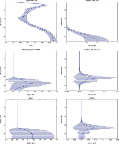
In order to examine the information content for cloudy and rainy profiles, we have taken a set of profiles from the 48 h forecast starting at 12 UTC on the 10 July 2006 over ocean and land surfaces, with a simple description of surface emissivity. For this forecast range, a set of 613 profiles has been selected by S. Di Michele (personal communication), and we have chosen 25 of them that are sampled over contrasted regions over the globe (Fig. 1). Indeed, the computation of the Jacobians with the ARTS model, being done in finite differences, is rather time consuming. Figure 2 shows the mean profiles of temperature, water vapour, cloud liquid water, cloud ice water, rain and snow and their associated variability (represented by the standard deviation over the set of 25 profiles). It appears that despite the reduced size of the database, the variability of these parameters shows that they cover a wide range of contrasted situations. The precipitation fluxes R have been converted into mass contents q with a formula proposed by Geer et al. (2009) that is consistent with PSD and fall speed velocity assumptions made in the RTTOV-SCATT radiative transfer model.

Fig. 1. Set of 613 profiles over oceans taken from an ECMWF 48 h forecast starting on 10 July 2006 small (black squares). The large red squares indicate the location of the 25 selected profiles.

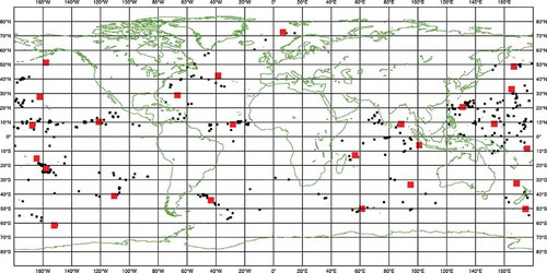
Fig. 2. Mean and standard deviation of the 25 profiles of the database for temperature (a), water vapour (b), cloud liquid water (c), cloud ice water (d), rain (e) and snow (f).

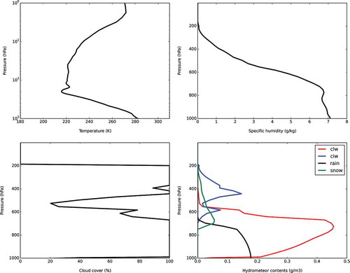
For illustration purposes during the course of the paper, a specific profile has been arbitrarily chosen and is presented in Fig. 3. This profile corresponds to a point located in the stormtrack region of the Northern Pacific ocean (48.68°S, 166.77°E). It is representative of oceanic mid-latitude convection leading to large cloud amounts extending throughout the troposphere, with warm, mixed and cold phases. Temperatures are close to 280 K near the surface and decrease linearly in log-pressure scale up to the tropopause located near 200 hPa (minimum temperature of 210 K). Then, in the stratosphere the temperature increases again to reach a value of 270 K at the stratopause (1 hPa). The specific humidity profile has rather constant value close to 7 gkg^–1 up to 700 hPa corresponding to the isotherm 0° where the atmosphere is saturated and rain water contents are around 1.8 g/m³, with large cloud water contents (up to 0.45 g/m³). Then, specific humidity decreases up to 200 hPa where it reaches very small values. The cloud mixed phase is located between 750 and 400 hPa. The ice water profile is characterised by two maxima, a first one around 450 hPa (0.15 g/m³) corresponding to a high level opaque cloud reaching the tropopause, and a second one (0.8 g/m³) at the top of a low level opaque cloud (identified by the minimum value in cloud cover around 570 hPa). The snow profile has negligible values at cloud top (200 hPa) that increase linearly towards the surface with a melting layer around 700 hPa. The rain only layer extends from 750 hPa to the surface.

Fig. 3. Temperature (a), water vapour (b), fractional cloud cover (c), hydrometeor contents (d) for the 13^th profile of the database.

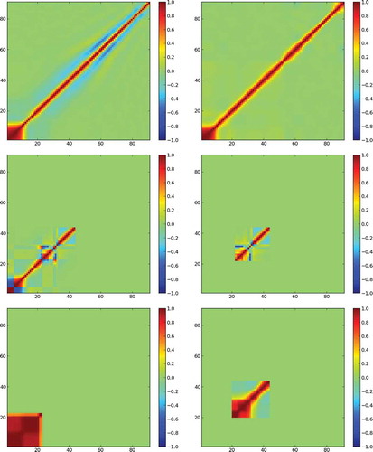
The variances for hydrometeors that have been obtained after applying the linearised moist physics to the -matrix for temperature and specific humidity (eq. (9)) revealed somewhat unrealistic vertical profiles with very large and localised values around cloud boundaries induced by the breakdown of the tangent linear approximation in such regions (not shown). As a consequence, for all hydrometeors, the standard deviation of background errors has been set to 40% of the actual value of the profile, in order to reflect the rather high level of uncertainty in the forecast of these variables in NWP models. On the other hand, the vertical auto-correlations for the 6 atmospheric variables of interest (Fig. 4) reveal patterns that are consistent with published studies (Ménétrier and Montmerle, 2011; Michel et al., 2011). The correlations for T and q exhibit patterns similar to those obtained from various ensemble methods (e.g. Derber and Bouttier, 1999), in particular with negative correlations near adjacent levels for temperature and large vertical correlations in the boundary layer. When examining the correlations for hydrometeors, a block diagonal structure is evidenced corresponding to the layers where a given type is present. The cloud ice water correlations are divided in two blocks separated by the level where the profile has a mimimum value. The cloud liquid water correlations are divided in three major blocks, the first two at high levels have similar patterns to ice water. Indeed in this cold cloud region, liquid water, despite being very small, has non zero values (from a continuous dependency of the mixed phase with temperature in the cloud scheme in order to increase its derivability). In the warm cloud layer, non-diagonal elements are present near cloud base. For rain water contents, strong vertical correlations are induced by the non-local effect of falling hydrometeors affecting the whole precipitating layer. The same pattern is also found for snow water contents but only in the bottom part of the layer where the amounts are the largest associated with significant terminal fall speeds.

Fig. 4. Correlation of background errors for temperature (a), water vapour (b), cloud liquid water (c), cloud ice water (d), liquid precipitation (e) and solid precipitation (f) for the 13^th profile of the database.

The cross-correlation matrices between variables computed from eq. (9) are not used since the information content is performed for each variable independently. This choice comes from the fact that a global information content study would heavily rely on correlations between variables in the B matrix and on the relative sizes of the variances that have a rather high level of uncertainty.

3.4. Jacobians of radiative transfer model

The elements of the matrix H have been computed for the 25 profiles of the database and the six variables of interest. An example of Jacobians over ocean surface is illustrated in Fig. 5 for the 251 line channels corresponding to the selected profile (Fig. 2) with respect to temperature (a), specific humidity (b), cloud liquid water (c), cloud ice water (d), rain water content (e), and snow water content (f). The Jacobians have been scaled by a perturbation taken equal to 10% of the profile value (except for temperature where a 1 K value is chosen) in order to produce a sensitivity in Kelvins (change in ):

(10)

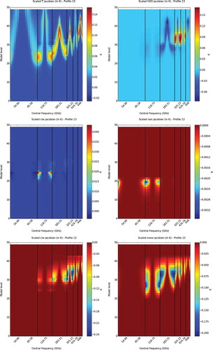
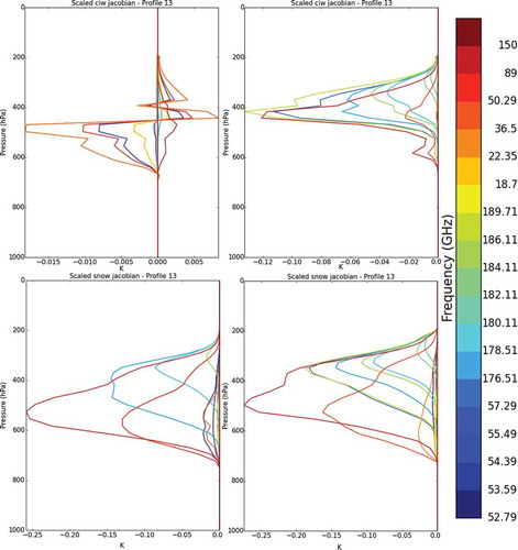
Fig. 5. Scaled Jacobians in K for cloud liquid water (a), liquid precipitation (b), cloud ice water (c) and solid precipitation (d) for the 13^th profile of the database in oxygen and water vapour absorption bands (see Table 1).

where x is either T, , , , or .

This allows the comparison of Jacobians for the different variables that would otherwise have different units.

These Jacobians are presented in Fig. 5 for the oxygen and water vapour absorption lines over an ocean surface. The Jacobians in absorption lines are similar over land surfaces (not shown). The Jacobians for temperature show positive values in the oxygen absorption lines at 60 GHz, 118 GHz and 425 GHz (Fig. 5a). The values are non-negligible from the lower troposphere (800 hPa) to high levels, particularly for the 60 and 118 GHz lines. In the water vapour bands (183, 325 and 448 GHz), the Jacobians have rather large values in the mid-troposphere (larger than in the oxygen bands) but they extend only up to the upper troposphere corresponding to the region with significant water vapour concentrations. The Jacobians for water vapour have negative values at high levels at 183 GHz near the centre of the absorption line (Fig. 5b). The profile being saturated over most of the troposphere, the sounding channels have there a negligible sensitivity. Frequencies above 200 GHz, in particular the 325 GHz band, reveal positive Jacobians above cloud top around model level 30 (200 hPa). Such behaviour is rather different from the one in clear sky situations.

The Jacobians for cloud liquid water show the largest values at the top of the warm cloud layer in the 118 GHz absorption band, but the absolute perturbations are rather small in terms of brightness temperatures (around 0.03 K) (Fig. 5c). The sensitivity of ice water content is important for frequencies around 183 GHz and above, with maximum values peaking higher up when moving towards higher frequencies (Fig. 5d). One can notice that in the 325 GHz absorption band the Jacobian can reach values up to 0.24 K. Rainfall Jacobians have negative values in the far wings of the 60 GHz and the 118 GHz bands but by small amounts (0.003 K) (Fig. 5e). The sensitivity decreases for higher frequencies. Snowfall Jacobians have large values in the wings of the absorption band at 118 GHz, 183 GHz and above, with the height of the maximum sensitivity increasing with frequency (Fig. 5f). The size of these perturbations is rather large (around 0.2 K).

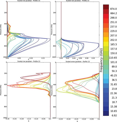
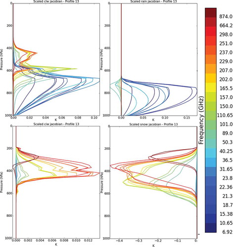
The Jacobians for the 25 window channels are presented as individual profiles in Figs. 6 (ocean surface) and 7 (land surface). The list of the 25 channels is given in Table 2. Over an ocean surface the Jacobians for cloud liquid water have a vertical structure that reflects the shape of the profile with maximum values around 650 hPa (top of the warm cloud layer) for low frequency channels from 6.9 to 50 GHz. Jacobians for rain water show a rather similar shape for channels between 6.9 and 50 GHz. Higher frequencies, between 89 and 110 GHz, reveal non negligible negative values around 700 hPa being the signature of scattering processes, and the Jacobians for frequencies higher than 150 GHz are negligible. Jacobians for cloud ice water content have large negative values in the middle of the cold cloud layer for frequencies around 250 GHz (up to −0.3 K) and smaller maximum values higher up (−0.2 K) for the two highest frequencies. Frequencies below 90 GHz lead to negligible Jacobians. Snow Jacobians have a rather broad vertical structure with significant negative values over the whole snow layer for frequencies above 90 GHz.

Fig. 6. Scaled Jacobians in K for cloud liquid water (a), liquid precipitation (b), cloud ice water (c) and solid precipitation (d) for the 13^th profile of the database in window regions (see Table 2), over ocean surface.

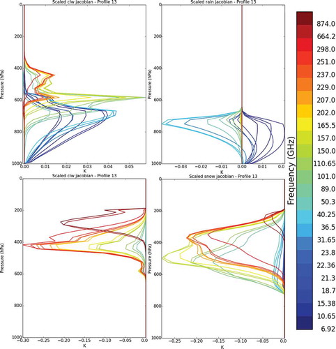
When considering the Jacobians over land (Fig. 7), significant differences appear with respect to the patterns noticed in Fig. 6 (ocean surface). These Jacobians exhibit smaller values (around 0.04 K and 0.02 K for cloud liquid water and rain, respectively) for low frequencies channels between 6.295 and 23.8 GHz. It reflects the fact that the surface emission provides a stronger contribution to the top of the atmosphere radiance, thereby reducing the sensitivity of the emission from liquid hydrometeors. For cloud liquid water, the maximum values of the Jacobians are reached at frequencies between 50 and 100 GHz, which have a maximum value of 0.05 K for frequencies between 89 and 150 GHz. For rain, the Jacobians are maximum in absolute value (−0.04 K) at frequencies around 50 GHz at the top of the rain layer. On the contrary, Jacobians for solid hydrometeors are not affected by the surface type.

Fig. 7. Scaled Jacobians in K for cloud liquid water (a), liquid precipitation (b), cloud ice water (c) and solid precipitation (d) for the 13^th profile of the database in window regions (see Table 2), over land surface.

3.5. Comparison between ARTS and RTTOV Jacobians

In order to gain confidence on the Jacobians of ARTS that have been computed in finite differences for the hydrometeors, they are compared for the profile displayed in Fig. 3 (13^th profile of the database) to the Jacobians from the RTTOV-SCATT radiative transfer model obtained through an analytical derivation of the numerical code (adjoint technique) as explained in Bauer et al. (2006a). We have used the version 11 of RTTOV-SCATT, and chosen the SSMI/S F18 radiometer that has a set of 24 window and sounding channels between 19 and 183 GHz. The geometry is set with an incidence angle of 53° and the surface emissivity is specified to a value of 0.6. The scattering processes are accounted for differently by the two models: with the Delta-Eddington approximation for RTTOV-SCATT and with the DOIT scheme for ARTS. The radiative properties of hydrometeors have also differences. Similar to ARTS, RTTOV-SCATT considers spherical particles for liquid and ice cloud water contents with respective densities of 1000 and 900 kg/m³. The PSDs have modified Gamma shapes. Rain particles are represented in both models by liquid water spheres following a Marshall–Palmer exponential distribution. The radiative properties for these spherical particules are computed from the Mie theory. The main difference is for snow particules that have been recently modified by Geer and Baordo (2014) from ‘soft spheres’ to particules of various shapes where the Discrete Dipole Approximation (DDA) method is used to compute the scattering properities (Liu, 2008). Moreover, the PSD is defined from the normalised distribution concept of Field et al. (2007). Given the fact that the snow particles are ice spheres in the ARTS simulations, we have selected in the database of Liu (2008) the particule with similar shape and density: the block hexagonal column.

A set of 18 channels from SSMI/S for which it is possible to find rather close ones from the 276 HYMS channels (named hereafter ‘SSMIS surrogate’) has been selected. In practice we have discarded the six mesospheric channels around the 63.28 and 60.792 GHz absorption bands. Since HYMS is a single-side band radiometer, it means that individual brightness temperatures on each side of absorption lines are computed with the SSMIS surrogate whereas an average value is given for the SSMI/S channels simulated with RTTOV-SCATT. As before, we compare scaled Jacobians. As expected for the T and q channels (not shown) there is good level of agreement in terms of size and shape of the Jacobians between ARTS and RTTOV-SCATT. The Jacobians between ARTS and RTTOV-SCATT are rather similar for liquid cloud and rain (Fig. 8) but the size of for the 18.70 GHz frequency is larger by 70% with ARTS. Regarding solid hydrometeors (Fig. 9), the choice of the block hexagonal column for precipitating particles leads to similar values of for the two schemes, the largest value being at 150 GHz, followed by the 183 GHz channels showing sounding effects and by the 89 GHz channel with the largest peaking sensitivity corresponding the maximum of snow content. These channels exhibit also significant Jacobian values for with ARTS (up to 0.12 K) whereas they have almost negligible values with RTTOV-SCATT, where the largest sensitivity is for a much lower frequency at 36.5 GHz. Even though it is not possible to know where is the truth, it is very likely that the extremely weak scattering by cloud ice with RTTOV-SCATT is not realistic (there should be some continuity with precipitating particles with similar shape and density and that induce significant scattering displayed by the large negative values of the Jacobians). On the other hand, with ARTS the scattering by cloud ice is almost as strong as the one for precipitating ice, despite considering much smaller particles. This tends to indicate that the scattering by cloud ice is somewhat overestimated with ARTS.

Fig. 8. Comparison of scaled Jacobians in K for cloud liquid water (top) and rain (bottom) between SSMI/S computed with RTTOV-SCATT (left column) and SSMI/S ‘surrogate’ computed with ARTS (right column) for the 13^th profile of the database (set of 18 sounding and window channels between 18.7 and 183 GHz).

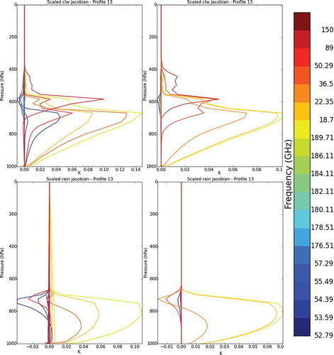
Fig. 9. Comparison of scaled Jacobians in K for cloud ice water (top) and solid precipitation (bottom) between SSMI/S computed with RTTOV-SCATT (left column) and SSMI/S ‘surrogate’ computed with ARTS (right column) for the 13^th profile of the database (set of 18 sounding and window channels between 18.7 and 183 GHz).

In conclusion, it appears that the Jacobians computed by ARTS compare rather well with the ones from RTTOV-SCATT for a range of frequencies between 18 and 183 GHz, for all variables but cloud ice water. The Jacobians appear too large for ARTS and too low for RTTOV-SCATT, even though it is not possible to provide strong scientific arguments to justify these statements. The scattering processes govern the size of the negative Jacobians for solid hydrometeors, and the ARTS choice for solid precipitation to consider ice spheres leads to rather large Jacobians for . Given these significant differences, a sensitivity study is undertaken hereafter to examine the impact of microphysical assumptions for hydrometeors in ARTS on the Jacobians and on the information contents.

4. Results on information content

4.1. Experimenal set-up with low frequencies

Before presenting results for a HYMS instrument, we have set-up a preliminary methodology similar to the one proposed by DMB2006 where they have examined the information content of channels between 1 and 200 GHz. Here we also restrict the information content to channels from HYMS below 200 GHz (211 channels). We have specified observation errors as proposed by DMB2006 to 1.5 K for all channels. In the clear-sky study of Mahfouf et al. (2015) it has been possible to prescribe more realistic errors based on innovation statistics from the global Météo–France data assimilation system. In cloudy situations, the use of innovation statistics is more difficult since they are dominated by displacement errors, leading to rather large values, whereas it should include only measurement and radiative transfer errors. Radiative transfer modelling errors are likely to increase with frequency given uncertainties associated to the scattering properties of solid hydrometeors. Such intuitive statement is not easy to translate in a quantitative manner; therefore, the observation error will be kept to 1.5 K throughout the study. The main objective of this validation step is to examine if despite the small amount of profiles, results obtained with a much larger database can be recovered. Such preliminary step should provide information on the robustness of the results presented afterwards with a HYMS instrument having frequencies up to 900 GHz.

Tables 3 and 4 show the 10 channels having the largest DFS values for the four hydrometeors over ocean and land surfaces, averaged over the 25 profiles. A number of results found by DMB2006 are recovered. The most informative channels for liquid water (cloud and rain) are between 30 and 40 GHz, and the 15.375 and 18.70 GHz frequencies over ocean surfaces and frequencies between 89 and 150 GHz over land surfaces. The low frequency channels at 6.9 GHz and 10.65 GHz present on Advanced Microwave Scanning Radiometers (AMSRs) are ranked 5 and 6 for liquid precipitation over oceans. For snow, new channels at 101 and 165.5 GHz, and window channels between 89 and 150 GHz appear to provide information on top of the 183 GHz absorption band. Ice water content has not been examined by DMB2006. Here the window region at 165.5 GHz complements the 183 GHz absorption band. What is also noticeable is the fact that the lower frequency channels explain a larger fraction of the total DFS for liquid hydrometeors than for solid hydrometeors. This result confirms the ‘well-known’ need for exploring higher frequencies in order to retrieve information on ice and snow in cloudy systems (Buehler et al., 2007, 2012). The specification of the surface does not affect the most informative channels for ice and snow, associated with frequencies above 89 GHz. These high frequencies are sensitive to scattering at upper altitudes, thereby reducing the sensitivity to the surface. Regarding liquid hydrometeors, the fractional DFS for the first 10 channels is significantly reduced when going from an ocean surface to a land surface. Indeed, low frequencies are sensitive to both the emission of land and liquid hydrometeors. This leads to reduced values of Jacobians for liquid water and rain over land as shown in Fig. 7. In the following, results are only shown over ocean surfaces since they appear to be more robust (i.e. overall agreement with 25 profiles with results presented by DMB2006).

Table 3. Summary of the ten most informative channels on cloud liquid water , liquid precipitation , cloud ice water and solid precipitation for a microwave radiometer spanning frequencies between 6.9 and 200 GHz with a 53° incidence angle over oceans for a set of 25 constrated profiles, together with the corresponding fractional DFS, over ocean surfaces. This configuration is similar to the experimental set-up of DMB2006. The frequencies in bold are not available on current or future instruments. Other frequencies are available on current and future instruments, in italic for window regions and in roman for absorption band

Rank
1	36.50	31.65	192.91	150
2	31.65	36.50	193.31	192.91
3	40.25	40.25	192.51	157
4	18.7	18.7	192.11	192.51
5	101	10.65	191.71	101
6	89.00	6.925	191.31	192.11
7	15.375	15.375	165.5	165.5
8	150	23.80	190.91	89
9	110.65	21.30	190.51	193.71
10	23.8	22.355	190.11	191.71
DFS (%)	73.19	89.64	43.69	41.81

Table 4. Same as Table 3 over land surfaces

Rank
1	101	18.7	192.91	150
2	36.5	15.375	193.31	192.91
3	40.25	23.8	192.51	157
4	31.65	101	192.11	192.51
5	89	21.3	191.71	101
6	150	89	191.31	192.11
7	110.65	31.65	165.5	165.5
8	157	6.375	190.91	191.71
9	18.7	40.25	190.51	89
10	15.375	36.5	190.11	193.31
(%)	64.41	63.81	43.6	41.81

4.2. Experimental set-up with high frequencies

The previous experimental set-up has been extended to the 276 HYMS channels spanning frequencies up to 874 GHz. Results are presented in Table 5 for the 20 channels having the largest DFS values for the four hydrometeors and also for temperature and specific humidity. Regarding liquid cloud and rain water contents, the dominance of low frequency channels (below 110 GHz) in terms of information content is confirmed since the first 10 selected channels are unchanged with respect to the previous set-up (ignoring frequencies above 200 GHz). Four new frequencies that will not be on EPS-SG instruments – 15.37, 40.25, 101 and 110.65 GHz –provide large information content on these two parameters. For cloud liquid water, window channels between 6 and 165.5 GHz are ranked between 10 and 20. It appears that there are only three sounding channels (around 118 GHz) in the 20 first channels. On the other hand besides low frequency channels (<50 GHz) informative about rain water contents, the wings of the absorption band at 118 GHz and window channels between 89 and 150 GHz are selected between rank 10 and 20 in agreement with Bauer et al. (2005). When examining solid hydrometeors, a totally different channel selection compared to the previous set-up is obtained. It appears that for ice water content, the highest frequencies are the most informative ones: 874, 664, window channels between 200 and 300 GHz, channels in the absorption line at 325 and 425 GHz, in agreement with previous studies (Buehler et al., 2007, 2012). A significant number of channels on board EPS-SG are selected by the DFS method (showing indirectly that the proposed methodology is sound despite various limitations discussed previously). For snow, window channels between 100 and 250 GHz and channels around 325 and 425 GHz appear to be the most informative ones (8 channels among the first 20). The most informative channels for specific humidity are very similar to those obtained in clear-sky conditions with a 53° geometry (Mahfouf et al., 2015): low frequency window channels around the weak absorption band at 22.235 GHz and the sounding channels at 183 GHz and 325 GHz, with also a few window channels above 200 GHz. On the other hand, for temperature, the most informative channels, that were found in the 55 GHz absorption band, are now located around the 448 GHz frequency (water vapour absorption band) and in the 183 GHz absorption line. From the important water load in cloudy situations, the sensitivity of these water vapour channels on temperature is enhanced, especially in the water vapour absorption lines at 183 and 450 GHz. Given the fact that sounding channels are sensitive to both water vapour and temperature it can be difficult to separate their contribution in an inversion procedure and the use of channels allows to disentangle this ambiguity. Mahfouf et al. (2015) already discussed this issue in clear-sky conditions. However, in cloudy regions where specific humidity is constrained by its value at saturation, extracting information on temperature from water vapour channels could make more sense since in that case, the only degree of freedom is temperature (assuming that the cloudy region remains in the inversion process).

Table 5. Summary of the twenty most informative channels on cloud liquid water , liquid precipitation , cloud ice water , solid precipitation , specific humidity q and temperature T for an HYMS instrument spanning frequencies between 6.9 and 874 GHz with a 53° incidence angle over oceans for a set of 25 constrated profiles, together with the corresponding fractional DFS, over ocean surfaces. The frequencies in bold are not available on current instruments. Other frequencies are available on current and future instruments, in italic for window regions and in roman for and absorption bands

Rank					T	q
1	36.50	31.65	874	150	447	21.3
2	31.65	36.50	664.2	251	450	22.355
3	40.25	40.25	298	157	446	23.8
4	18.7	18.7	251	101	451	182.91
5	101	10.65	334.15	334.15	182.11	334.15
6	89	6.925	229	298	449	664.2
7	15.375	15.375	431.76	416.76	183.71	181.71
8	150	23.8	335.15	229	181.31	315.15
9	110.65	21.3	315.15	89	445	183.71
10	23.8	22.355	237	335.15	182.51	174.91
11	10.65	89	417.76	315.15	180.91	251
12	157	101	432.76	110.65	180.51	874
13	6.925	110.65	456	207	444	298
14	21.3	113.75	207	237	184.91	174.11
15	22.355	113.95	431.76	165.5	183.31	173.31
16	113.75	114.15	333.15	417.76	184.11	18.7
17	113.95	114.35	455	318.15	180.11	322.15
18	165.5	114.55	418.76	40.25	452	321.15
19	114.15	50.3	202	319.15	229	173.71
20	229	150	316.15	332.15	182.91	182.51
DFS (%)	85.75	96.17	70.69	48.96	24.43	40.60
	27	11	49	90	154	94

When examining the link between the fractional DFS value and the number of corresponding HYMS channels, most of the information on liquid cloud and rain can be obtained with a reduced set of channels (27 and 11 respectively in order to reach a 90% value). More channels are required to reach the same fractional DFS value for cloud ice and snow (49 and 90 respectively). When examining T and q it appears that many more channels are required compared to clear-sky situations in order to extract useful information in cloudy regions (e.g. 154 channels for temperature compared to 70 channels as found in Mahfouf et al. (2015)).

4.3. Sensitivity study to microphysical properties

The comparison between ARTS and RTTOV-SCATT Jacobians for SSMI/S channels has revealed that microphysical assumptions impact the Jacobians of hydrometeors. Here we examine further this sensitivity. In the baseline set-up (named ‘all’ afterwards), previously described in Section 3.1, scattering properties of all hydrometerors are computed using Mie theory and a spherical shape. Three additional set-up are tested (named ‘mix1’, ‘mix2’ and ‘mix3’ afterwards), that have considered two databases of scattering properties for frozen hydrometeors. A database proposed by Liu (2008) provides properties of various shapes, sizes and temperature intervals for frequencies between 6.295 and 340 GHz. Another database for similar properties has been proposed by Hong et al. (2009) with different choices for the particle shapes and over a different frequency domain (ranging from 89 to 874 GHz). For solid precipitating particles, scattering properties are chosen to be ‘sector-snowflakes’ from the Liu database and to be ‘aggregates’ from the Hong database. The PSD is prescribed from the parameterisation of Field et al. (2007) fitted for tropical regions. For cloud liquid droplets, rain and cloud ice, scattering properties are still computed under the assumption of spherical shapes using Mie theory. The PSD is specified by a modified Gamma law for cloud liquid droplets and cloud ice, and a Marshall-Palmer (exponential) distribution for rain. The density is set to 900 kgm^–3 for cloud ice. These two databases have been used to define three experimental set-ups for the Jacobians ranging from 6.295 to 874 GHz: ‘mix1’ corresponds to Liu microphysics below 89 GHz and Hong microphysics above 89 GHz, ‘mix2’ corresponds to Liu microphysics below 183 GHz and Hong microphysics above 183 GHz, and ‘mix3’ corresponds to Liu microphysics below 340 GHz and Hong microphysics above 340 GHz. The various set-ups are summarised in Table 6.

Table 6. Summary of the microphysical properties of the various experimental set-ups. The particule size distributions are defined as: H98 (Hess et al., 1998), MP48 (Marshall and Palmer, 1948), MH97 (McFarquhar and Heymsfield, 1997), MGD (Modified Gamma Distribution), F07 (Field et al., 2007). For non-spherical particles, the ‘sector snowflake’ is chosen for the Liu-DDA and the ‘aggregate’ for the Hong-DDA

Setup	Main features
all	Mie spheres for ql (H98), qr (MP48), qi (MH97) Mie spheres for qs (MP48)
mix 1	Mie spheres for ql (MGD), qr (MP48), qi (MGD) Liu-DDA ≤ 89 GHz and Hong-DAA > 89 GHz for qs (F07)
mix 2	Mie spheres for ql (MGD), qr (MP48), qi (MGD) Liu-DDA ≤ 183 GHz and Hong-DAA > 183 GHz for qs (F07)
mix 3	Mie spheres for ql (MGD), qr (MP48), qi (MGD) Liu-DDA ≤ 340 GHz and Hong-DAA > 340 GHz for qs (F07)

The Jacobians for hydrometeors are shown in Fig. 10 (window channels) for hydrometeors with ‘mix1’ set-up for the profile of interest. The Jacobians are almost identical with ‘mix2’ and ‘mix3’ set-ups (not shown). The Jacobians for liquid water (cloud and rain) are very similar to the Jacobians with the ‘all’ set-up. For cloud liquid water, the high frequency windows channels above 89 GHz have larger values at higher altitudes, in the mixed phase layer. The differences with the ‘all’ set-up are more pronounced for solid hydrometeors. The Jacobians for cloud ice have small negative values at 664 and 874 GHz around 350 hPa and positive values between 200 and 300 hPa. They have their largest positive values, but rather small in absolute terms (0.01 K), at altitudes around 400 hPa for frequencies between 89 and 300 GHz and are negligible below 89 GHz. The Jacobians for snow have very large negative values (up to −0.4 K) for high frequencies above 150 GHz. The highest frequencies at 664 and 874 GHz show a peak between 200 and 300 hPa, at the top of the cloud layer. The frequencies between 150 and 300 GHz have a peak between 300 and 400 hPa and the lower frequencies have a peak at lower altitudes, around 500 hPa.

Fig. 10. Scaled Jacobians in K for cloud liquid water (a), liquid precipitation (b), cloud ice water (c) and solid precipitation (d) for the 13^th profile of the database in window regions (see Table 2), for ‘mix1’ set-up over ocean surface.

The results of channel selections with the new microphysics are compared with the ones obtained with the ‘all’ set-up in Table 7. For liquid hydrometeors (cloud and rain) almost no changes are noticeable when using different microphysical assumptions. For cloud ice, the most informative channel is still the 874 GHz window channel with the ‘mix’ set-ups. On the other hand, the channel at 664.2 GHz, that was the second most informative with the ‘all’ set-up, is ranked much lower with ‘mix2’ and ‘mix3’ set-ups, and is even absent from the most informative frequencies with the ‘mix1’ set-up. Similarly, the information content of the 425 GHz absorption line decreases with the ‘mix’ set-ups. For solid precipitation, the most informative channel becomes the frequency at 874 GHz with the ‘mix’ set-ups whereas it was not highly ranked with the ‘all’ set-up. One can also notice that the 664 GHz contains significant information on solid precipitation with the ‘mix’ set-ups contrary to the ‘all’ set-up.

Table 7. Summary of most informative channels on cloud liquid water , liquid precipitation , cloud ice water , solid precipitation , specific humidity q and temperature T for an HYMS instrument spanning frequencies between 6.9 and 874 GHz with a 53° incidence angle over oceans for a set of 25 constrated profiles, for a set of four microphysical properties summarised in Table 6

Setup
all	30–40 GHz	30–40 GHz	664–874 GHz	89–157 GHz
	15–23 GHz	6–23 GHz	200–300 GHz	200–300 GHz
	89–157 GHz	89–150 GHz	325 GHz	325 GHz
	118 GHz	118 GHz	425 GHz	425 GHz
mix1	30–40 GHz	30–40 GHz	874 GHz	874 GHz
	89–157 GHz	6–23 GHz	200–300 GHz	150–300 GHz
	118 GHz	89–150 GHz	325 GHz	664 GHz
	15–23 GHz	118 GHz	150–200 GHz	325 GHz
mix2	30–40 GHz	30–40 GHz	874 GHz	874 GHz
	89–157 GHz	6–23 GHz	200–300 GHz	150–300 GHz
	118 GHz	89–150 GHz	325 GHz	664 GHz
	15–23 GHz	118 GHz	664 GHz	325 GHz
mix3	30–40 GHz	30–40 GHz	874 GHz	874 GHz
	89–157 GHz	6–23 GHz	200–300 GHz	150–250 GHz
	118 GHz	89–150 GHz	325 GHz	664 GHz
	15–23 GHz	118 GHz	664 GHz	325 GHz

4.4. Comparison with SSMI/S and EPS-SG instruments

In order to stress the interest of a future hyper-spectral microwave sensor (HYMS), its information content on hydrometeors and also on temperature and specific humidity is compared to the current capabilities of microwave radiometers by considering the SSMI/S instrument with 18 channels (5 in the 55 GHz band, 7 in the 183 GHz band, and 6 in window regions between 18.70 and 150 GHz). These channels are selected among the 276 initial candidates. Then, another comparison is done with the conical scanning microwave instruments on board the future EPS-SG platform. The spectral bandwidths are kept unchanged with respect to the initial selection of 276 channels and the viewing angle remains 53°. We have retained 23 channels for ICI, 28 for MWI and 43 for the two instruments (given the redundancy of some channels).

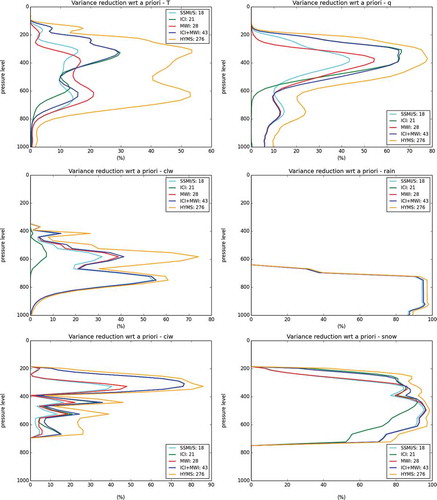
First, we examine the variance reduction that would be induced on the background accuracy by the assimilation of the selected channels for the profile of interest with the ‘all’ set-up (Fig. 3). The variance reduction is computed as:

where is the variance of analysis error and is the variance of background error.

If the observed radiances do not bring any information with respect to the a priori, the value of VR is zero. If the observations would lead to a perfect atmospheric state the value of VR would be one (or 100%). The variance reduction for the six atmospheric quantities is shown in Fig. 11 for the 13^th profile of the database, with the ‘all’ set up. Five curves are displayed: the variance reduction with the whole set of HYMS channels (276), with the 43 channels of MWI + ICI, with individual instruments (MWI, ICI) and with SSMI/S. For all variables, the HYMS sounder is the one leading to the largest variance reduction. With respect to SSMI/S, it appears that the benefit of future and hypothetical instruments (MWI, ICI, HYMS) will not bring additional information on rainfall. HYMS has a small added value due to the channels at 15.375 and 40.25 GHz. Similarly, the added value of HYMS with respect to MWI+ICI will be small for snow, even though the benefit with respect to SSMI/S, coming both from ICI at high levels and MWI at lower levels, is quite clear. The ICI instrument is not informative about cloud liquid water, whereas the MWI has performances similar to SSMI/S for this quantity. A number of window channels present on HYMS but not on MWI could provide additional information in the mixed phase region (top of the warm cloud layer) (40.25, 15.37, 101 and 110.65 GHz). The ice water content at high levels is much improved by the ICI instrument whereas MWI has a similar behaviour to SSMI/S. On the other hand the addition of the 874 GHz frequency increases the variance reduction at that levels with HYMS. An additional significantly larger benefit of HYMS with respect to MWI+ICI is also noticed between 700 and 400 hPa. Regarding temperature, the variance reduction affects the atmosphere between 800 and 200 hPa and is maximum for HYMS due to its large number of channels each one bringing a small piece of information (as displayed by the small amount of fractional DFS with only 20 channels). The reduction is the largest in the upper troposphere near 300 hPa thanks to the 874 and 664 GHz channels and in the mid-troposphere around 600 hPa from the other window channels corresponding to altitudes where the Jacobians are the largest (not shown). Finally, the variance reduction for water vapour is only significant in the cold part of the cloud from to channels sensitive to ice water content, as highlighted by the large contribution of ICI.

Fig. 11. Variance reduction (expressed in percentage) for temperature (a), water vapour (b), cloud liquid water (c), cloud ice water (d), liquid precipitation (e) and solid precipitation (f) induced by the assimilation of SSMI/S, MWI, ICI, MWI + ICI and HYMS microwave instruments for the 13^th profile of the database and the ‘all’ set-up for microphysics.

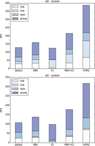
Figure 12 presents the total DFS summed over all profiles of the database for SSMI/S, the EPS-SG instruments and HYMS with 276 channels, for microphysical set-ups ‘all’ and ‘mix1’ (since as shown in Table 7 there are no significant differences between ‘mix1’ ‘mix2’ and ‘mix3’). For the ‘all’ set-up, the conclusions are similar, but more robust, to the ones obtained when examining the variance reduction over a single profile (Fig. 11). The information content provided by HYMS for the various atmospheric variables is larger than that of SSMI/S or MWI+ICI for the two microphysics set-ups. For the ‘all’ set-up, the added value from MWI+ICI is clearly on cloud ice and snow whereas it is rather marginal for liquid water and rain. On the contrary, with the ‘mix1’ set-up the contribution of MWI + ICI is rather weak for cloud ice but more significant for snow. This highlights the uncertainties regarding the specification of microphysical properties for solid hydrometeors. For liquid hydrometeors the contribution of MWI + ICI is similar to that of SSMI/S, but HYMS increases the total DFS by about a factor of two for rain and cloud liquid water. The fact that the ICI instrument is dedicated to solid hydrometeors is clearly displayed by the diagnostic with the ‘all’ and ‘mix1’ set-ups. There is a clear benefit of HYMS for all variables, that could be much larger than the improvement brought by going from a SSMI/S instrument to the combined MWI+ICI radiometers. The total is increased by a factor of 1.7 with respect to MWI+ICI and by a factor of 3 with respect to SSMI/S. The total for cloud ice is rather low for the ‘mix1’ set-up with all instruments including HYMS but the corresponding DFS for solid precipitation is significantly increased. This result indicates that the separation between snow and ice is strongly dependent upon the assumptions made on PSDs and scattering properties within the radiative transfer model.

Fig. 12. Degrees of Freedom for Signal (DFS) for the following hydrometeors: cloud liquid water (clw), cloud ice water (clw), liquid precipitation (rain), solid precipitation (snow). They are given for various configurations of present and future microwave radiometers, for ‘all’ (top panel) and ‘mix1’ (bottom panel) set-ups. Each DFS has been computed over a set of 25 atmospheric profiles. The corresponding microphysical properties are summarised in Table 6.

5. Conclusions

This study has examined the information content on temperature, water vapour and hydrometeors (cloud, ice, rain, snow) provided by a theoretical hyper-spectral microwave sensor HYMS over the frequency range between 6.9 and 874 GHz (millimetre and sub-millimetre wavelengths), that has been compared to microwave frequencies of SSMI/S and future similar instruments onboard EPS-SG. The results give insight on the use of future microwave instruments for NWP. A database of profiles from ECMWF model short-range forecasts has been used with corresponding background error covariance matrices, partly computed from linearised moist physical parameterisation schemes. The optimal estimation theory has allowed to assess the information content of channels in oxygen and water vapour absorption lines and of window channels located in the weak absorbing regions of the microwave spectrum. The radiative transfer model ARTS has been used as an observation operator to compute the Jacobians of each channel for each atmospheric quantity. Since ARTS is a line-by-line model where scattering is solved with a rather computationally expensive algorithm (DOIT) and for which the linearised versions are not available, the computations of the Jacobians by the brute force method (finite differences) have been cumbersome, preventing from examining more than 25 profiles, that however have been chosen in order to have a maximum of variability of cloud properties. In order to evaluate the relevance of this small set of profiles, we have performed an information content study similar to the one of DMB2006 that has considered more than 10 000 atmospheric profiles (but limited to 200 GHz in terms of microwave spectrum). Results appear to be more robust over oceans than over land due to the larger variability of continental surface emissivities. A comparison has also been done between the Jacobians obtained by ARTS in finite differences and the ones from RTTOV-SCATT from an analytical derivation of the numerical code (adjoint technique). There is an overall agreement between the Jacobians except for cloud ice water where the scattering by RTTOV-SCATT appears negligible (very small Jacobians) and could be too large for ARTS, despite similar hypotheses for particle shape and density (but with different PSDs). As a result we have undertaken a sensivity study of the Jacobians and information content to the microphysical properties (particle size distributions and scattering parameters)

The most informative channels over frequencies from 6 to 874 GHz include mostly low frequency channels for liquid hydrometeors (below 50 GHz), with an additional information brought by the 118 GHz oxygen absorption line. For solid hydrometeors, the most informative channels are the high frequency window channels at 874 and 664 GHz, and between 200 and 300 GHz, with the absorption lines at 325 and 425 GHz. The window channels between 89 and 200 GHz are also informative for snow. The sensitivity of the results to the microphysical properties has been examined by considering three additional set-ups with different size distributions and different scattering properties. The most informative channels are the same for liquid hydrometeors, with only few high frequency channels (above 150 GHz). The most informative channels for solid hydrometeors are the window channels at 874 and 664 GHz. On the other hand, according to the set of chosen microphysics, the importance of ice cloud can be strongly reduced at the expense of solid precipitation.

Regarding the information content brought by HYMS, compared to current and future microwave instruments, the new window channels between 15 and 110 GHz for rain and up to 150 GHz for liquid water would lead to a non-negligible increase whereas the MWI+ICI instruments do not appear to bring significant information with respect to SSMI/S for these variables. On the other hand, the benefit of frequencies above 200 GHz (874 and 664 GHz window channels, 325, 425 and 448 GHz absorption bands) for ice and snow water contents is clearly shown for both MWI + ICI and HYMS with respect to SSMI/S. These known results have led to the design of the future spaceborne instruments but are confirmed with our methodology that is based on linear estimation theory with a reduced number of profiles. New frequencies proposed in the candidate channels of HYMS could also be useful for solid hydrometeor retrievals. Nevertheless, the amount of information that can be retrieved from each instrument strongly depends on the microphysical properties of hydrometeors, especially for snow and ice. With a different set-up, the DFS for cloud ice can be strongly reduced for ICI and HYMS and the one for snow strongly enhanced. Regarding temperature in cloudy regions, the most informative channels are located around the water vapour 448 and 183 GHz bands due to the important water load. However, the number of channels to explain 90% of the DFS is rather large (154). Since the atmosphere is saturated, it removes one degree of freedom in terms of dependency of the brightness temperatures, but introduces additional ones on hydrometeors that could dominate the signal. Since the current method deals with each variable independently it is blind to physical water changes induced by cloud microphysics. Rather similar conclusions hold for water vapour but in that case the selected channels are consistent with the ones retained in clear sky conditions (Mahfouf et al., 2015).

In conclusion, our methodology has been able to recover over ocean surfaces known results regarding the interest of low microwave frequencies (<200 GHz) for liquid hydrometeor information content (Bauer et al., 2005; DMB2006) and high microwave frequencies (>200 GHz) for solid hydrometeor information content that have led to the definition of the ICI radiometer on-board EPS-SG (Buehler et al., 2007). New channels proposed in a HYMS with 276 channels would increase the information content on hydrometeors. The new frequencies that would bring most information on hydrometeors are: (1) window channels at 40.25-, 15.375-, 101-, 110.65-GHz for liquid hydrometeors; (2) window channels at 251 and 298 GHz, plus channels in the absorption lines at 425 GHz for solid hydrometeors. The differences obtained over land with a set of 25 profiles against the ones from DMB2006 reveal that it would be relevant to examine the information content over a larger database of profiles over land, since the use of a single value of surface emissivity is not sufficient to capture the large variability of continental surface microwave emissivities. Over oceans, we are confident that our conclusions are robust since we have performed a sensitivity study with only 12 profiles and similar conclusions have been reached. The possibility of retrieving information on temperature and specific humidity in cloudy regions with a HYMS has been shown but it is not clear if this result is an artifact of the methodology. Therefore it seems more prudent to select channels for these variables on the basis of clear-sky information contents (Mahfouf et al., 2015).

Acknowledgements

The study was funded by an ESA contract N 4000105721/12/NL/AF entitled ‘Use of spectral information at microwave region for numerical weather prediction’. We would like to thank Chung-Chi Lin and Ville Kangas for their coordination and supervision of the project. We are also grateful to Filipe Aires and Catherine Prigent for leading the scientific activities during the course of the project. The atmospheric profiles and the background errors were kindly provided by Sabatino Di Michele.

Disclosure statement

No potential conflict of interest was reported by the authors.

Additional information

Funding

This work was supported by the ESA [N 4000105721/12/NL/AF].

References

- Aires, F., Prigent, C., Bernardo, F., Jiménez, C., Saunders, R. and co-authors. 2011. A tool to estimate land-surface emissivities at microwave frequencies (TELSEM) to use in numerical weather prediction. Quart. J. Roy. Meteor. Soc. 137(656), 690–699. DOI:10.1002/qj.v137.656.
- Bauer, P. and Di Michele, S. 2007. Mission Requirements for a Post-EPS Microwave Radiometer. Post-EPS EUMETSAT Contract No EUM/CO/06/1510/PS.
- Bauer, P., Geer, A. J., Lopez, P. and Salmond, D. 2010. Direct 4D-Var assimilation of all-sky radiances: part I. Implementation. Quart. J. Roy. Meteor. Soc. 136, 1868–1885. DOI:10.1002/qj.659.
- Bauer, P., Lopez, P., Benedetti, A., Salmond, D., Saarinen, S. and co-authors. 2006b. Implementation of 1D+4D-Var assimilation of precipitation affected microwave radiances at ECMWF. Part II: 4D-Var. Quart. J. Roy. Meteor. Soc. 132, 2307–2332. DOI:10.1256/qj.06.07.
- Bauer, P., Moreau, E., Chevallier, F. and O’Keeffe, U. 2006a. Multiple scattering microwave radiative transfer for data assimilation applications. Quart. J. Roy. Meteor. Soc. 132, 1259–1281. DOI:10.1256/qj.05.153.
- Bauer, P., Moreau, E. and Di Michele, S. 2005. Hydrometeor retrieval accuracy using microwave window and sounding channel observations. J. Appl. Meteor. 44, 1016–1032. DOI:10.1175/JAM2257.1.
- Blackwell, W. J., Bickmeier, L. J., Leslie, R. V., Pieper, M. L., Samra, J. E. and co-authors. 2011. Hyperspectral microwave atmospheric sounding. IEEE Trans. Geosci. Rem. Sens. 49, 128–142. DOI:10.1109/TGRS.2010.2052260.
- Boukabara, S. A. and Garrett, K. 2011. Benefits of a hyperspectral microwave sensor. IEEE Sens. Proc. 1881–1884. DOI:10.1109/icsens.2011.6127367.
- Buehler, S., Eriksson, P., Kuhn, T., von Engeln, A. and Verdes, C. 2005. ARTS, the atmospheric radiative transfer simulator. J. Quant. Spectrosc. Radiat. Transf. 91, 65–93. DOI:10.1016/j.jqsrt.2004.05.051.
- Buehler, S. A., Defer, E., Evans, F., Eliasson, S., Mendrok, J. and co-authors. 2012. Observing ice clouds in the submillimeter spectral range: the CloudIce mission proposal for ESA’s Earth Explorer 8. Atmos. Meas. Tech. 5, 1529–1549. DOI:10.5194/amt-5-1529-2012.
- Buehler, S. A., Eriksson, P. and Lemke, O. 2011. Absorption lookup tables in the radiative transfer model ARTS. J. Quant. Spectrosc. Radiat. Transf. 112(10), 1559–1567. DOI:10.1016/j.jqsrt.2011.03.008.
- Buehler, S. A., Jiménez, C., Evans, K. F., Eriksson, P., Rydberg, B. and co-authors. 2007. A concept for a satellite mission to measure cloud ice water path, ice particle size, and cloud altitude. Q. J. R. Meteorol. Soc. 133, 109–128. DOI:10.1002/qj.v133:2+.
- Buehler, S. A., von Engeln, A., Brocard, E., John, V. O., Kuhn, T. and co-authors. 2006. Recent developments in the line-by-line modeling of outgoing longwave radiation. J. Quant. Spectrosc. Radiat. Transf. 98(3), 446–457. DOI:10.1016/j.jqsrt.2005.11.001.
- Cardinali, C. 2009. Monitoring the observation impact on the short-range forecast. Q. J. R. Meteorol. Soc. 135, 239–250. DOI:10.1002/qj.v135:638.
- Chevallier, F., Di Michele, S. and McNally, A. P. 2006. Diverse profile datasets from the ECMWF 91-level short-range forecasts. NWP SAF Satellite Application Facility for Numerical Weather Prediction, No. NWPSAF-EC-TR-010.
- Collard, A. D. 2007. Selection of IASI channels for use in numerical weather prediction. Q. J. R. Meteorol. Soc. 133, 1977–1991. DOI:10.1002/qj.v133:629.
- Davis, C. P., Evans, K. F., Buehler, S. A., Wu, D. L. and Pumphrey, H. C. 2007. 3-D polarised simulations of space-borne passive mm/sub-mm midlatitude cirrus observations: a case study. Atmos. Chem. Phys. 7, 4149–4158. DOI:10.5194/acp-7-4149-2007.
- Derber, J. and Bouttier, F. 1999. A reformulation of the background error covariance in the ECMWF global data assimilation system. Tellus A 51, 195–221. DOI:10.1034/j.1600-0870.1999.t01-2-00003.x.
- Di Michele, S. and Bauer, P. 2006. Passive microwave radiometer channel selection based on cloud and precipitation information content. Q. J. R. Meteorol. Soc. 132, 1299–1323. DOI:10.1256/qj.05.164.
- Emde, C., Buehler, S. A., Davis, C., Eriksson, P., Sreerekha, T. R. and co-authors. 2004. A polarized discrete ordinate scattering model for simulations of limb and nadir longwave measurements in 1D/3D spherical atmospheres. J. Geophys. Res. 109(D24), D24207. DOI:10.1029/2004JD005140.
- English, S., McNally, T., Bormann, N., Salonen, K., Matricardi, M., co-authors. 2013. Impact of Satellite Data. ECMWF Tech. Memo No 711, 48 pp.
- Eriksson, P., Buehler, S., Davis, C., Emde, C. and Lemke, O. 2011. ARTS, the atmospheric radiative transfer simulator, version 2. J. Quant. Spectrosc. Radiat. Transf. 112, 1551–1558. DOI:10.1016/j.jqsrt.2011.03.001.
- Eriksson, P., Ekström, M., Melsheimer, C. and Buehler, S. A. 2006. Efficient forward modelling by matrix representation of sensor responses. Int. J. Rem. Sens. 27(9), 1793–1808. DOI:10.1080/01431160500447254.
- Eriksson, P., Jamali, M., Mendrok, J., and Buelher, S. A. 2015. On the microwave optical properties of randomly oriented ice hydrometeors. Atmos. Meas. Tech., 8(9), 1913–1933. DOI:10.5194/amt-8-1913-2015.
- Field, P. R., Heymsfield, A. J. and Bansemer, A. 2007. Snow size distribution parameterization for midlatitude and tropical ice clouds. J. Atmos. Sci. 64, 4346–4365. DOI:10.1175/2007JAS2344.1.
- Fourrié, N. and Rabier, F. 2004. Cloud characteristics and channel selection for IASI radiances in meteorologically sensitive areas. Q. J. R. Meteorol. Soc. 130, 1839–1856. DOI:10.1256/qj.03.27.
- Fourrié, N. and Thépaut, J.-N. 2003. Evaluation of the AIRS near-real-time channel selection for application to numerical weather prediction. Q. J. R. Meteorol. Soc. 129, 2425–2439. DOI:10.1256/qj.02.210.
- Fox, S., Lee, C., Rule, I., King, R., Rogers, S. and co-authors 2014. ISMAR: a new submillimeter airborne radiometer. In: Proceedings of the 13th Specialist Meeting on Microwave Radiometry and Remote Sensing of the Environment (MicroRad), Pasadena, CA, 24–27 March 2014, 128–132.
- Geer, A. J. and Boardo, F. 2014. Improved scattering radiative transfer for frozen hydrometeors at microwave frequencies. Atmos. Meas. Tech. 7, 1839–1860. DOI:10.5194/amt-7-1839-2014.
- Geer, A. J. and Bauer, P. 2010. Enhanced Use of All-Sky Microwave Observations Sensivite to Water Vapour, Cloud and Precipitation. ECMWF Technical Memorandum N° 620, 41 pp.
- Geer, A. J., Bauer, P. and Lopez, P. 2010. Direct 4D-Var assimilation of all-sky radiances. Part II. Assessment. Quart. J. Roy. Meteor. Soc. 136, 1886–1905. DOI:10.1002/qj.681.
- Geer, A. J., Bauer, P. and O’Dell, C. W. 2009. A revised cloud overlap scheme for fast microwave radiative transfer. J. Appl. Meteor. Clim. 48, 2257–2270. DOI:10.1175/2009JAMC2170.1.
- Geer, A. J., Boardo, F., Bormann, N. and English, S. 2014. All-Sky Assimilation of Microwave Humidity Sounders. ECMWF Technical Memorandum No 741, 59 pp.
- Hess, M., Koepke, P. and Schult, I. 1998. Optical properties of aerosols and clouds: the software package OPAC. Bull. Am. Meteor. Soc. 79, 831–844. DOI:10.1175/1520-0477(1998)079<0831:OPOAAC>2.0.CO;2.
- Hong, G., Yang, P., Baum, B. A., Heymsfield, A. J., Weng, F. and co-authors. 2009. Scattering database in the millimeter and submillimeter wave range of 100–1000 GHz for nonspherical particles. J. Geophys. Res.: Atmos. 104(D6)114. DOI:10.1029/2008JD010451.
- Janisková, M. and Lopez, P. 2013. Linearized physics for data assimilation at ECMWF. In: Data Assimilation for Atmospheric, Oceanic and Hydrological Application (eds. S. K. Park and L. Xu) Vol. II, Springer-Verlag Berlin Heidelberg, pp. 251–286.
- John, V. O. and Buehler, S. A. 2004. The impact of ozone lines on AMSU-B radiances. Geophys. Res. Lett. 31, L21108. DOI:10.1029/2004GL021214.
- Karbou, F., Gérard, É. and Rabier, F. 2006. Microwave land emissivity and skin temperature for AMSU-A and -B assimilation over land. Q. J. R. Meteorol. Soc. 132, 2333–2355. DOI:10.1256/qj.05.216.
- Karbou, F., Rabier, F., Lafore, J.-P. and Redelsperger, J.-L. 2010. Global 4DVAR assimilation and forecast experiments using AMSU observations over land. Part II: impacts of assimilating surface-sensitive channels on the African monsoon during AMMA. Weather Forecast. 25, 20–36. DOI:10.1175/2009WAF2222244.1.
- Karbou, F., Rabier, F. and Prigent, C. 2014. The assimilation of observations from the advanced microwave sounding unit over sea ice in the French global numerical weather prediction system. Mon. Weather Rev. 142, 125–140. DOI:10.1175/MWR-D-13-00025.1.
- Kim, M.-J., Weinman, J. A., Olson, W. S., Chang, D.-E., Skofronick-Jackson, G. and co-authors. 2008. A physical model to estimate snowfall over land using AMSU-B observations. J. Geophys. Res. 113, D09201. DOI:10.1029/2007JD008589.
- Kuntz, M. and Höpfner, M. 1999. Efficient line-by-line calculation of absorption coefficients. J. Quant. Spectrosc. Radiat. Transf. 63, 97–114. DOI:10.1016/S0022-4073(98)00140-X.
- Lipton, A. E. 2003. Satellite sounding channel optimization in the microwave spectrum. IEEE Trans. Geosci. Rem. Sens. 41, 761–781. DOI:10.1109/TGRS.2003.810926.
- Liu, G. 2008. A database of microwave single-scattering properties for nonspherical ice particles. Bull. Am. Met. Soc. 89, 1563–1570. DOI:10.1175/2008BAMS2486.1.
- Lopez, P. 2011. Direct 4D-Var assimilation of NCEP stage IV radar and gauge precipitation data at ECMWF. Mon. Weather Rev. 139, 2098–2116. DOI:10.1175/2010MWR3565.1.
- Lopez, P. and Moreau, E. 2005. A convection scheme for data assimilation: description and initial tests. Quart. J. Roy. Meteor. Soc. 131, 409–436. DOI:10.1256/qj.04.69.
- Lorenc, A. C. and Marriott, R. T. 2014. Forecast sensitivity to observations in the met office global numerical weather prediction system. Q. J. R. Meteorol. Soc. 140, 209–224. DOI:10.1002/qj.v140.678.
- Mahfouf, J.-F., Birman, C., Aires, F., Prigent, C., Orlandi, E. and co-authors. 2015. Information content on temperature and water vapour from a hyper-spectral microwave sensor. Quart. J. Roy. Meteor. Soc. 141, 3268–3284. DOI:10.1002/qj.2608.
- Marshall, J. S. and Palmer, W. M. K. 1948. The distribution of raindrops with size. J. Meteorol. 5, 165–166. DOI:10.1175/1520-0469(1948)005<0165:TDORWS>2.0.CO;2.
- Martinet, P., Lavanant, L., Fourrié, N., Rabier, F. and Gambacorta, A. 2014. Evaluation of a revised IASI channel selection for cloudy retrievals with a focus on the Mediterranean basin. Q. J. R. Meteorol. Soc. 140, 1563–1577. DOI:10.1002/qj.2014.140.issue-682.
- McFarquhar, G. M. and Heymsfield, A. J. 1997. Parameterization of tropical cirrus ice crystal size distributions and implications for radiative transfer: results from CEPEX. J. Atmos. Sci. 54, 2187–2200. DOI:10.1175/1520-0469(1997)054<2187:POTCIC>2.0.CO;2.
- Ménétrier, B. and Montmerle, T. 2011. Heterogeneous background error covariances for the analysis and forecasts of fog events. Q. J. R. Meteorol. Soc. 137, 2004–2013. DOI:10.1002/qj.802.
- Michel, Y., Auligné, T. and Montmerle, T. 2011. Heterogeneous convective-scale background error covariances with the inclusion of hydrometeor variables. Mon. Weather Rev. 139, 2994–3015. DOI:10.1175/2011MWR3632.1.
- Mlawer, E. J., Payne, V. H., Moncet, J.-L., Delamere, J. S., Alvarado, M. J. and co-authors. 2012. Development and recent evaluation of the MT CKD model of continuum absorption. Philos. Trans. Roy. Soc. A 370(1968), 2520–2556. DOI:10.1098/rsta.2011.0295.
- Montmerle, T. and Berre, L. 2010. Diagnosis and formulation of heterogeneous background-error covariances at the mesoscale. Q. J. R. Meteorol. Soc. 136, 1408–1420. DOI:10.1002/qj.655.
- Prigent, C., Pardo, J. R. and Rossow, W. B. 2006. Comparisons of the millimeter and submillimeter bands for atmospheric temperature and water vapor soundings for clear and cloudy skies. J. Appl. Meteor. Clim. 45, 1622–1633. DOI:10.1175/JAM2438.1.
- Rabier, F., Fourrié, N., Chafa, D. and Prunet, P. 2002. Channel selection methods for infrared atmospheric sounding interferometer radiances. Q. J. R. Meteorol. Soc. 128, 1011–1027. DOI:10.1256/0035900021643638.
- Rodgers, C. D. 1996. Information content and optimisation of high spectral resolution measurements. In: Optical Spectroscopic Techniques and Instrumentation for Atmospheric and Space Research II. SPIE Proceedings (Eds. P. B. Hays and J. Wang) Vol. 2830, pp. 136–147. Denver, CO, United States, October 1996DOI:10.1117/12.256110.
- Rodgers, C. D. 2000. Inverse Methods for Atmospheres: Theory and Practice. World Scientific Publisher, Singapore.
- Rothman, L. S., Gordon, I. E., Babikov, Y., Barbe, A., Benner, C. D. and co-authors. 2013. The HITRAN2012 molecular spectroscopic database. J. Quant. Spectrosc. Radiat. Transf. 130, 4–50. DOI:10.1016/j.jqsrt.2013.07.002.
- Saunders, R. W., Hewison, T. J., Stringer, S. J. and Atkinson, N. C. 1995. The radiometric characterization of AMSU-B. IEEE Trans. Microwave Theor. Tech. 43(4), 760–771. DOI:10.1109/22.375222.
- Sreerekha, T. R., Buehler, S. A., O’Keeffe, U., Doherty, A., Emde, C. and co-authors. 2008. A strong ice cloud event as seen by a microwave satellite sensor: simulations and observations. J. Quant. Spectrosc. Radiat. Transf. 109(9), 1705–1718. DOI:10.1016/j.jqsrt.2007.12.023.
- Tompkins, A. M. and Janisková, M. 2004. A cloud scheme for data assimilation. Description and initial tests. Quart. J. Roy. Meteor. Soc. 130, 2495–2517. DOI:10.1256/qj.03.162.
- Van Vleck, J. H. and Huber, D. 1977. Absorption, emission and linebreadths: a semihistorical perspective. Rev. Mod. Phys. 49, 939–959. DOI:10.1103/RevModPhys.49.939.
- Xie, Y., Chen, J., Liu, D., Lv, C., Liu, K. and co-authors. 2013. Development and calibration of a K-band ground-based hyperspectral microwave radiometer for water vapour measurements. Prog. Electromagn. Res. 140, 415–438. DOI:10.2528/PIER13050704.