A weak-constraint 4DEnsembleVar. Part I: formulation and simple model experiments

ABSTRACT

4DEnsembleVar is a hybrid data assimilation method which purpose is not only to use ensemble flow-dependent covariance information in a variational setting, but to altogether avoid the computation of tangent linear and adjoint models. This formulation has been explored in the context of perfect models. In this setting, all information from observations has to be brought back to the start of the assimilation window using the space-time covariances of the ensemble. In large models, localisation of these covariances is essential, but the standard time-independent localisation leads to serious problems when advection is strong. This is because observation information is advected out of the localisation area, having no influence on the update.

This is part I of a two-part paper in which we develop a weak-constraint formulation in which updates are allowed at observational times. This partially alleviates the time-localisation problem. Furthermore, we provide—for the first time—a detailed description of strong- and weak-constraint 4DEnVar, including implementation details for the incremental form.

The merits of our new weak-constraint formulation are illustrated using the Korteweg-de-Vries equation (propagation of a soliton). The second part of this paper deals with experiments in larger and more complicated models, namely the Lorenz (1996) model and a shallow water equations model with simulated convection.

KEYWORDS:

• hybrid data assimilation
• ensemble-variational methods
• model error

1. Introduction

The 4-dimensional ensemble-variational data assimilation (DA) scheme, 4DEnVar, is a hybrid DA method currently used (and still being researched) in Numerical Weather Prediction (NWP), and it is at the forefront of the next-generation DA methods. As with other hybrid methods, the basic motivation behind 4DEnVar is to use the flow-dependent background error covariance matrix from sequential methods based on the Kalman Filter (KF)—like the Ensemble Transform Kalman Filter (ETKF, Bishop et al., 2001; Wang et al., 2004) and the Local Ensemble Transform Kalman Filter (LETKF, Hunt et al., 2007)—and apply it in the 4-dimensional variational framework (4DVar) first proposed by Le Dimet and Talagrand (1986), and studied in Talagrand and Courtier (1987). What makes 4DEnVar different from all other hybrids, however, is the fact that it alleviates the need to compute tangent linear models (TLM’s) and adjoint models (AM’s).

The use of ensemble information in a variational framework was proposed by Lorenc (2003) and Zupanski (2005). Since then, several formulations have been proposed, experimented on, and used by operational centres like the UK Met Office and the Canadian Meteorological Centre (Environ Canada). The idea of these hybrid methods is to overcome certain restrictions of the basic 4DVar, for instance, the use of a static background error covariance matrix, which is usually a climatological error covariance matrix . Although it is possible to generate slowly-varying ’s—e.g. difference covariances for different seasons–, the fast variations—e.g. those in the time-frame of an assimilation window—are not captured. Hence, climatological or slow-varying background matrices do not describe the flow-dependent errors of the day. Sequential ensemble-based methods, e.g. LETKF, can describe these features. Nonetheless, the sample covariances obtained in these ensemble methods—which we denote as —contain sampling errors and are seldom full rank, which is a problem climatological covariances do not have. It seems logical, then, to find ways to combine the advantages of both families of methods. Clayton et al. (2013) developed a hybrid 4DVar which combines the climatological background error covariance matrix with the flow dependent background error covariance matrix generated by the LETKF. Fairbarn et al. (2014) and Goodliff et al. (2015) then showed that a fully flow dependent background error covariance matrix outperforms a climatological or hybrid covariance in the 4DVar framework (4DVar-Ben). The former used model II of Lorenz (2005) with 240 variables, while the latter used the 3-variable Lorenz (1963) model with increasing non-linearity.

A non-trivial requirement for the implementation of 4DVar is generating TLMs and AMs for both the evolution and observation operators. Liu et al. (2008) developed the 4DEnVar technique, which overcomes this need. After a series of matrix transformations, the role of these matrices can be substituted by using four-dimensional space-time covariance matrices. In fact, the idea that an ensemble can be used to generate space-time covariances to use within an assimilation window was first proposed in the context of the Ensemble Kalman Smoother of Van Leeuwen and Evensen (1996) and Evensen and Van Leeuwen (2000).

A recent study by Lorenc et al. (2015) showed difficulties for the performance of 4DEnVar in larger systems, in comparison to that of 4DVar with hybrid background covariances. The authors point to the fact evolution and localisation of the covariance matrix do not commute. This means that it is not the same to evolve a localised a covariance matrix, or to evolve first and then localise.

So far, the work on 4DEnVar has been done considering a perfect model scenario, i.e. in a strong-constraint (SC) setting. In this work, we introduce a weak-constraint (WC) 4DEnVar. As explored by Tremolet (2006), the choice of control variables in WC4DVar is not unique. For reasons that will be thoroughly discussed in the paper, we use what we label an ‘effective model error formulation’, which stems from Tremolet’s (2006) constant bias formulation.

This work is presented in two parts. Part I describes the 4DEnVar formulation in detail. We discuss its advantages over traditional DA methods, as well as its short-comings. We pay special attention to the problem of localising time cross-covariances using static localisation matrices. We illustrate this problem by experimenting with the Korteweg de Vries (KdV) equation for the evolution of a soliton (see e.g. Zakharov and Faddeev, 1971). In part I we also introduce our WC4DEnVar and discuss a proper localisation implementation for this method. We show that performing updates at times other than the initial one (as one does in the SC case), partially alleviates the impact of incorrectly localised time cross-covariances. Simple DA experiments are performed in this model.

In part II we move into larger models. We start with a detailed exploration of parameters (e.g. observation frequency, observation density in space, localisation radii, etc) using the well-known Lorenz (1996) chaotic model. Then we use a modified shallow water equations (SWE) model with simulated convection (Wursch and Craig, 2014), which allows to test our method in a more realistic setting. This is a larger, more non-linear model and serves as a good test bed for convective data assimilation methods.

The layout of this paper is as follows. Sections 2 and 3 describe in details the methodology of the 4DEnVar framework. Section 2 covers the SC case, and in Section 3 we introduce our WC4DEnVar formulation. In Section 4 we use the KdV model and use it to illustrate the time evolution of the background error covariance matrix, as well as the problems that come from static localisation of cross-time covariance matrices. In Section 5 we perform some brief DA experiments. Section 6 summarises the work of this part.

2. The variational methods

2.1. Strong-constraint 4DVar

In this section we formulate the SC4DVar method, which forms the basis of any subsequent approximation. Consider the discrete-time evolution of a dynamical system determined by the following equation:

(1)

where is the vector of state variables, and is a map which evolves the state variables from time to time . For the moment, we consider this model to be perfect. The initial condition is not known with certainty, and can be considered a random variable (rv). In particular, we consider it to be a Gaussian rv, i.e. , where is a background value or first guess (usually coming from a previously generated forecast), and represents the background error covariance matrix, which is full rank and positive definite. One often replaces this matrix with a climatological background error covariance . There are several ways to obtain it (e.g. Parrish and Derber, 1981; Yang et al., 2006); see e.g. Bannister (2008) for a review.

The system is observed from time to time. For a given observational time, the observation equation is:

(2)

where is the vector of observations and is the observation operator. For simplicity we consider this operator constant through time. We use the term ‘observation period’ to denote the number of model time steps between consecutive observation vectors. The observations contain errors, which are represented by the rv . We consider this error to be Gaussian and unbiased: , where is the observation error covariance matrix.

Let us consider a given time span from to , which we label ‘assimilation window’. By incorporating information from the background at and the observations within this window, we can find a better estimate (analysis) for the value of the state variables at every time step . Since the model is perfect (SC4DVar), this reduces to finding the minimiser of a cost function that only depends on the initial condition :

(3)

where the first term corresponds to the contribution from the background and the second term corresponds to the contributions from observations. To avoid an extra index to distinguish between time instants with and without observations, we introduce the indicator function if is a time instant with observations, and if is a time instant with no observations.

The complexity in minimising (3) depends on the particular characteristics of the operators and . For general non-linear operators, is not convex and may have multiple minima, leading to a difficult minimisation process. Another issue comes from the condition number of . If this is large (i.e. the largest and smallest eigenvalues of are separated by orders of magnitude), numerical minimisation methods can require many iterations for convergence. To solve these problems one can use a preconditioned formulation to reduce the ellipticity of the cost function. Moreover, an incremental formulation can be used to perform a quadratic approximation the original cost function, leading to a problem with a unique minimum. This linearisation process can be iterated several times; these iterations are the so-called outer loops.

To write down the preconditioned incremental problem, let us express the initial condition as an increment from the original background value, and then precondition the increment:

(4)

where is the new control variable. Since is full rank and symmetric, one can find the (unique) symmetric square root without further complications. In this case, and . Then, one can approximate (3) by performing the following first order Taylor expansion:

where

(5)

is the departure of the observations with respect to the evolution of the background guess throughout the assimilation window. To compute these departures one uses the full (generally non-linear) evolution and observation operators. We notice that two matrices appear in the equation. These are the TL observation operator

(6)

and TLM of the discrete-time evolution operator

(7)

which is also known as the transition matrix from time to time . Both Jacobian matrices are evaluated with respect to the reference trajectory, i.e. the evolution of . Then, the pre-conditioned incremental form of SC-4DVar can be written as:

(8)

This is a quadratic equation which only depends on . In order to find its global minimum it suffices to find the gradient and set it equal to zero. The gradient of (8) is:

(9)

2.2. Strong-constraint 4DEnsembleVar

Writing TLM’s and AM’s for large and complex models is a complicated process. Moreover, the calculations involving both TLM’s and AM’s are computationally expensive. To alleviate these problems, 4DEnVar was introduced. Once more, let us consider an assimilation window from to , with several observational times equally distributed throughout the assimilation window. Consider that at time we have an ensemble of forecasts. This ensemble can be initialized at time with the analysis coming from an LETKF running in parallel to the 4DEnVar system. At any time we can express the background (or forecast) ensemble as the matrix:

(10)

from which an ensemble mean can be calculated at any time as:

(11)

where is a vector of ones. Finally, a normalized ensemble of perturbations can be computed as

(12)

In the EnVar framework we replace the background error covariance at the beginning of an assimilation window by the sample estimator:

(13)

In applications (e.g. NWP) it is often the case that , so is a low rank non-negative definite matrix, which has consequences we discuss later. A straightforward implementation of 4DEnVar is to equate . Then, we can do the following substitution:

(14)

An advantage of using ensemble estimators is that we can directly construct the ensemble of perturbations using the full non-linear operators and the ensemble in the way described, e.g., in Hunt et al. (2007). Briefly, one can write:

(15)

and it follows that:

(16)

and the gradient (9) can be written simply as:

(17)

and it should be clear that up to this moment we have not applied localisation. Hence the size of the control variable we solve for is .

A graphic summary of the SC4DEnVar process is depicted in Fig. 1. This simple schematic depicts the three-stage-process of SC4DEnVar. These are:

Fig. 1. Schematic depicting the three stage process of 4DEnVar. In part i an ensemble of ‘free’ (DA-less) trajectories of the model is run for the length of the assimilation window. In part ii the 4DVar minimisation process is performed using 4-dimensional cross-time covariances instead of tangent linear and adjoint models. In part iii an LETKS is run to the end of the assimilation window to create new initial conditions for the next window. The mean of this LETKS is replaced by the solution of 4DEnVar, considered to be more accurate.

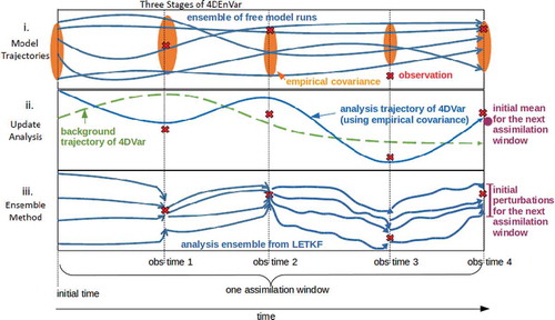
i. First an ensemble of ‘free’ (DA-less) trajectories of the model is run for the length of the assimilation window. In NWP applications these trajectories are available since meteorological centres often have an ensemble forecast system.

ii. Second, the 4DVar minimisation process is performed using 4-dimensional cross-time covariances instead of TLM’s and AM’s. These cross-time covariances are computed from the family of free model runs of step i.

iii. Finally an LETKF (or any other ensemble KF) is run throughout the assimilation window to create new initial conditions for the next window. The mean of this LETKF is replaced by the solution of 4DEnVar, considered to be more accurate, i.e. the ensemble keeps its perturbations but it is re-centred.In this implementation, two assimilation systems need to be operated and maintained. There are other hybrid systems such as ECMWF’s ensemble DA system (Bonavita et al., 2012) which are self-sufficient, but they require the use of TLM’s and AM’s.

2.2.1. Applying localization

The quality of depends on the size of the ensemble. In particular, the quality of this estimator is quite poor when , or at least when it is smaller than the number of positive Lyapunov exponents in the system. A common practice is to eliminate spurious correlations by tampering the covariance matrix in the following manner (Whitaker and Hamill, 2002):

(18)

where denotes the Schur (element-wise) product, and is the so-called localisation matrix. The element is a decreasing function of the physical distance between grid points and . This is usually chosen as the Gaspari and Cohn (1999) compact support approximation to a Gaussian function.

In the gradient of the 4DVar cost function the product appears. In the ensemble setting, this product corresponds to , which can be computed and localised as:

(19)

which clearly requires a new matrix . For linear observation operators, the two localisation matrices are related simply as:

(20)

In order to write a localised version of (17) we require factorisations of both and . Buehner (2005) showed that one can get the factorisation

(21)

with

(22)

where the operator converts a vector into a matrix with said vector in its main diagonal and zeros elsewhere, is the square root of the , and . If the localisation only depends on the distance amongst grid points (i.e. there is not a special cross-variable localisation or vertical localisation) then , i.e. simply the number of grid points. Constructing can be done relatively easily via the following eigenvalue decomposition:

(23)

where is the unitary matrix of eigenvectors, and is a diagonal matrix containing the eigenvalues, and we have used the fact that is symmetric. Then:

(24)

If there are many variables per grid point, the decomposition can be performed by blocks. Also, it is often more convenient to work with a truncated localisation matrix with a given rank . This is discussed thoroughly in Appendix 1.

In the case of we need to write

(25)

with defined as before, and

(26)

where can easily be found as:

(27)

The actual implementation we use can be found in Appendix 1. It is closer to Lorenc (2003) and his so-called -control-variable formulation. Wang et al. (2007) proved that both formulations are equivalent.

2.2.2. Localisation in 4-dimensional cross-time covariances

Recall that we have to compute the product , which we replace by the sample estimator . Note that these covariances involve both the ensemble of state variables at time 0, and the ensemble of equivalent observations at time . Hence, different products should be localised with different localisation matrices:

(28)

Computing the static matrix is not difficult since it requires no information about the flow. However, there is no simple way of computing an optimal , since that would require taking into account the dynamics of the model. Generally, the implementation of SC4DEnVar uses for all time steps, which can result in an unfavourable performance with respect to SC4DVar (Lorenc et al. 2015). This is a crucial impediment for an adequate performance of SC4DEnVar with long assimilation windows. We will illustrate this issue in detail in Section 4, where we provide a concrete example.

2.3. Weak-constraint 4DVar

Let us revisit the discrete-time dynamical system studied before, but this time not assuming perfect model. The evolution equation becomes:

(29)

In this case is the map which evolves the state variables from time to time , and is a rv representing the model error. Let it be a Gaussian rv centred in zero (unbiased), i.e. where is the model error covariance matrix.

Tremolet (2006) provides a detailed account on the way to include the model error term into the 4DVar cost function. As he points out, there is no unique choice for control variable in this case. For our implementation, we choose a variation of what he labels model-bias control variable. Consider the following representation of the true value of the state variables at any time:

(30)

i.e. the state variables at any time can be written as the perfect evolution of the initial condition—given by the discrete-time map —plus an effective model error , which contains the accumulated effect of the real mode errors at each model step, along with their evolution. While Tremolet (2006) considered the effective model error to be constant for all observational times throughout the assimilation window (), we let it vary for different observational times.

For a linear model , the relationship between the statistical characteristics of the model error at every time step from to and those of the effective model error at can be found in the following way:

(31)

which is not an easy relationship, but later we will discuss simpler—and more modest—ways to approximate . For the moment we consider this error to be unbiased.

Let us express the WC4DVar cost function as:

(32)

where the function now depends upon and . Notice that all the (perfect) model evolutions start at time . This is why we have chosen (30) as a definition of our control variables. If we chose the model error increment for every time step , we would find a cost function with terms of the form , i.e. perfect model evolutions initialised at different model time steps, where contains the effects of all for previous model time steps. This would complicate the problem considerably, especially when using ensembles.

As in the 4DVar case, we can write down a preconditioned incremental formulation. Recalling that:

(33)

we express the control variables as:

(34)

which allows to perform the following first order Taylor expansion:

(35)

where as in the SC case. The incremental preconditioned form of the cost function for WC4DVar is:

(36)

We can write the gradient as the following vector:

(37)

where the control variable is .

It would seem that the size of the problem has grown considerably with respect to the SC case. Nonetheless, let us look closer at the structure of (37). Remember that only if belongs to those time steps with observations (a set we denote as ), and otherwise. Hence the sum in the first block-element of only has (total number of observational times) terms. For all the other block elements we have two terms: the first corresponding to the model error contribution and the second contribution to the observational error contribution. For all time steps with no observations, this later term is null. In these time steps there is nothing to make the model error to be different from its background value, which was zero by construction. Therefore for all time steps without observations, and consequently we can redefine our control variable from to . Hence, the number of control variables—as well as the computational cost of the problem—scales with the number of observational times included in a given assimilation window.

2.4. Weak-constraint 4DEnsembleVar

As in the SC case, we want to find a way to avoid computing TLM’s and AM’s. In the absence of localisation, we substitute and to yield the gradient of the cost function as:

(38)

where the control variable is . As in the SC case, the actual implementation details can be found in Appendix 1.

In the SC case, the influence from observations at different times leads to a single increment that is computed at initial time , and the analysis trajectory comes from the evolution of the new initial condition. Roughly speaking, the information from observations at time impact changes at time via the covariance . Since we do not have we simply use . This is not too inaccurate for observations occurring relatively close (in a time-distance sense) to the beginning of the assimilation window. However using instead of can lead to considerable errors as grows. Hence, this issue is of particular importance for long assimilation windows with observations close to the end of the window.

In the WC formulation we propose, the impact of an observation at time influences the state variable at and at time . So although we still have an incorrectly localised expression of the form , we also have a correctly localised term , where obviously . We have not solved the problem of localisation, but we try to ameliorate it by allowing for increments at time steps in which observations occur.

The way our formulation works, we have jumps (from background to analysis) at the initial time and at the time of the observations. We have not experimented with how to get a smooth trajectory for the whole assimilation window. A first approach would be to modify the initial conditions, and then distribute the updates at observational times amongst the time steps between observations, following a procedure similar to the Incremental Analysis Update of Bloom et al. (1996). This would avoid the sharp jumps from background to analysis at the times of the observations.

2.5. A note on

We have not said anything about the computation of , i.e. the covariance matrix of the effective model error . In principle, it could be calculated if we had access to two ensembles: one evolved with no model error using (1): , and one evolved with model error using (29): . For any time we can use the expression (30) to write the imperfect state in terms of the perfect state at that time plus an effective error :

(39)

We can compute the first two moments of this error as:

(40)

and the previous expressions can be approximated by evaluating sample estimators:

(41)

There are two issues to do with these calculations. First of all, we need two ensembles running at the same time. This is not too demanding; in fact we could divide a moderate size ensemble into two groups and run each of these groups with and without model error respectively. The major complication, however, is the evaluation of

(42)

in an efficient way. Some of the difficulties include the size of the resulting matrix, as well as the rank of the matrix. We have not done exploration in this direction. Instead we have chosen a rather simple parametrisation of this error as:

(43)

which can be interpreted as considering the accumulated model error to behave like the Wiener process. This is exact for a linear model with , i.e. when the evolution model is the identity. A more precise approximation—or indeed an efficient way to compute the actual value—is beyond the scope of this paper.

3. Illustration of the time-propagation of information: TLM vs 4D cross-time covariances

3.1. The KdV equation

In this section we illustrate the effects of using a static localisation matrix to localise time cross-covariances. We perform experiments using the Korteweg de Vries (KdV) system as model. The KdV equation is a non-linear partial differential equation in one dimension:

(44)

where denotes time, is the spatial dimension, and is a one-dimensional velocity field. This equation admits solutions called solitons, which correspond to the propagation of a single coherent wave, see e.g. Shu (1987) or Zakharov and Faddeev (1971).

This system has been used before for DA experiments in the context of feature DA and alignment error (e.g. Van Leeuwen, 2003; Lawson and Hansen, 2005). This system can be challenging for DA, since the propagation of coherent structures renders the linear and Gaussian assumptions in both the background and observational error to become less accurate. Nonetheless, the system is suited to show the emergence of asymmetric off-diagonal elements in the time cross-covariance matrices. Hence, we will use it for illustrative purposes and simple DA experiments. More detailed experiments are shown in part II of this paper with more appropriate models.

We reduce (44) into an ordinary differential equation (ODE) by discretising into grid points separated by , and perform a central and -order-accurate finite-difference approximation to both the dispersion and advection terms (after writing the latter in conservative form). Denoting and , we can write:

(45)

We choose grid points and , and allow for periodic boundary conditions, i.e. , where denotes the modulo operation. We use a -order Runge-Kutta method with time step to numerically integrate (45) in time. This integration renders a discrete-time map .

The initial condition of a perfect soliton is given by:

(46)

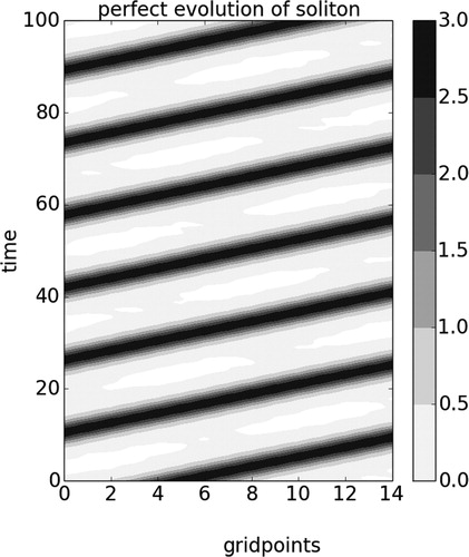
where is the center of the soliton at , and corresponds to the maximum velocity of the soliton. We choose (the propagation speed) which, combined with our steps and , yield a Courant number . Figure 2 is a Hovmoller plot showing the time evolution of the soliton through the domain. The horizontal axis represents different grid points, the vertical axis represents time (evolving from bottom to top), and the shading is proportional to the velocity at each grid point.

Fig. 2. Hovmoller plot showing the perfect evolution of a soliton produced by a numerical integration of the KdV equation over a periodical domain of 15 grid points.

For our experiments we require the discrete-time TLM (or transition matrix) of the model. We first obtain the continuous-time TLM . This is a hollow circulant matrix in which the row has all elements equal to zero except for:

(47)

where we recall that the indices are modular. Obtaining the transition matrix from the continuous-time TLM involves a straightforward solution of a matrix differential equation, see e.g. Simon (2006).

3.2. Covariance propagation

Let us start by obtaining the nature run of our system. As initial condition we use the profile described in (46), and we evolve the model until (i.e. model steps). The result of this run is illustrated in Fig. 2, this model run will later be used as the nature—or true—run of our DA experiments. The soliton propagates from left to right of the domain, taking about (time steps) to complete a loop around the domain.

We now examine the time propagation of a given . We construct this matrix following the method of Yang et al. (2006), which we describe briefly in Appendix 2. We obtain a circulant matrix, which normalized values for the row are:

(48)

Since we have the transition matrix of the model, we can explicitly compute both the covariance of the state at any time as:

(49)

and the cross-covariance between time and time as:

(50)

We evaluate both (50) and (49) for different lead times , and we plot these matrices in Fig. 3. Each individual panel is a covariance matrix, the horizontal and vertical axes are grid point locations. Let us start with the top row, which shows for different lead times (one for every column). The initial covariance is the circulant matrix shown in (48), but as the time increases we notice that off-diagonal features become more prominent. We notice a region of high values (shown in blue) developing above the main diagonal and the appearance of negative values (shown in white) along the main diagonal. The resulting matrices are not symmetric starting from , and this asymmetry grows as time passes. This is particularly evident after 10 and 15 steps.

Fig. 3. Analytical evolution of the covariance and cross-time covariance for the KdV model for different times (columns). The horizontal and vertical axes of each panel are the grid point locations. The first row shows and the second shows its localised version. The third row shows and the fourth shows its localised version.

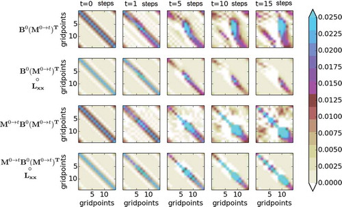
The third row shows for different lead times . In this case, all the matrices are symmetric by construction. There is a development of (symmetric) off-diagonal negative elements (shown in white), but most of the information remains concentrated close to the main diagonal. The magnitude of the matrix elements increases as time passes. As expected uncertainty grows in time.

Recall that we computed both and using and the actual transition matrix . The objective of 4DEnVar, however, is to compute these quantities using ensemble estimators, which contain spurious correlations if the ensemble size is small and lead to the need for localisation. The second and fourth rows of figure show the effect of localisation of and respectively, using a localisation matrix which follows a Gaspari and Cohn (1999) function with half-width grid points (centred in the main diagonal). As we can see in row 2, the localised versions of can lose most of the important information, and this problem becomes more pronounced as the time lag increases. The localised versions of , shown in the bottom row, lose less information, since the most distinguishable features were close to the main diagonal.

To appreciate better the effect of localisation with different half-widths, in Fig. 4 we depict the values of the row of the covariance matrices. The left panel of the first row shows . Each one of the different lines shows a different lead-time. Consider we are observing all variables, and look at the red line in the figure. We see a peak corresponding to grid point 10: this means that, for a lead-time of 15 time steps, the most useful information to update grid point 6 (at ) comes from the observation at grid point 10. This is no surprise, since the general direction of the flow is from left to right. Actually, for all lead-times we see that the most important information to update grid point 6 comes from observations in the grid points to the right. When localising the covariances this information is lost. This is not too crucial for relative large-scale localisation cases (middle column), but becomes very evident for strict localisation (right column). In both of these panels, the shape of the localisation function is shown in light gray for reference.

Fig. 4. Elements of the 6th row of the matrices (top row) and (bottom row), for different times (different colors). The first column shows the unaltered elements, while the middle and right columns show these elements after being localised using Gaspari-Cohn functions of different half-widths (gray lines).

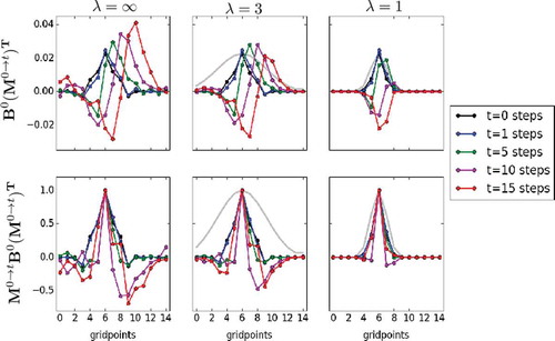
The left panel of the second row of Fig. 4 shows the of (actually we normalise and create a correlation-type matrix for ease of comparison, since the magnitudes in this matrix grow with time), and again different lines show a different lead-times. In all cases the dominant element is that corresponding to grid point 6. New features do develop (with respect to the original , i.e. the black line), but none is dominant. When localising with both a large- (middle column) and small- (right column) scale the information is not lost as crucially as before.

4. DA experiments under a perfect scenario

4.1. Setup

For these experiments, we extend the nature run generated before until (i.e. we have model steps). We create synthetic observations by taking the value of the variables at all grid points and all model time steps, and adding an uncorrelated random error with zero mean and , with . For the experiments we use subsets of these observations, both in time and space.

We observe every grid point; hence we have observed grid points and unobserved grid points. This sparse observational density (in space) makes the situation challenging, and the quality of the off-diagonal elements in the covariance matrices are quite important to communicate information from observed to unobserved variables. We experiment with several observational periods. We report the results of 3 cases: observations every 2 model steps, every 5 model steps, and every 10 model steps.

We test the following formulations: 3DVar, SC4DVar, ETKS, LETKS, SC4DEnVar and LSC4DEnVar. The L at the beginning of the EnVar methods denote the localised versions. ETKS and LETKS (S for smoother instead of filter) denote the ‘no-cost smoother’ versions of both ETKF and LETKF (see Kalnay and Yang, 2010 for a description).

Even though the nature run is generated with a perfect model, we also use WC methods for the sake of comparison. We use the effective error WC4DVar, as well as WC4DEnVar and LWC4DEnvar. In this case, we model the (fictitious) effective model error as a zero-center Gaussian rv with .

For the ensemble and hybrid methods we use a tiny ensemble size of . With this choice we try to mimic realistic situations where . This chosen value of should render low-quality sample estimators. The adaptive inflation of Miyoshi (2011) is used, with an initial value of . Inflation is generally applied in the following manner:

(51)

but following Miyoshi (2011), the inflation values are different for each grid point and it evolves with time.

For the localised methods, a Gaspari-Cohn function with half-width is used. We explored several values and kept the optimal one, which depends on the period of observations in each experiment. For the localised EnVar methods, we truncated the localisation matrix at 11 eigenvalues. Truncation with 9 to 15 kept eigenvalues was tried and gave similar results (not shown).

For the variational and hybrid methods, we use one observational time per assimilation window. We use the incremental pre-conditioned forms discussed earlier, and we do not use outer loops in any of these methods. We later performed experiments with 2 observational times per assimilation window and this did not change the main results (hence not shown).

4.2. Results

The results of these experiments are depicted in Figs. 5–7. Each figure has 3 columns and 2 rows. The top row corresponds to results of observed grid points, while the bottom row corresponds to results of unobserved grid points. Three panels are shown in each case:

Fig. 5. Using different DA methods in the KdV model for an observation period of 2 model steps. The left panels show the time evolution of the nature run (black line) and the analysis trajectories generated by different DA methods (color lines). The top row shows the case of grid point 1 (observed variable, observations are represented with gray circles), while the bottom row shows the case of grid point 3 (unobserved variable). The middle panels show the time evolution of the analysis RMSE. The top panel corresponds to observed variables, while the bottom panel corresponds to unobserved variables. For both cases, the horizontal gray line is the standard deviation of the observational error. The right panels show summary statistics for observed (top panel) and unobserved variables (bottom panel). We show intervals containing the first, second (median) and third quartiles of the analysis RMSE distribution in time.

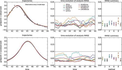
Fig. 6. Same as Fig. 5 but with an observational period of 5 model time steps.

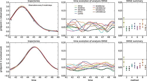
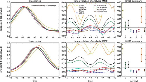
Fig. 7. Same as Fig. 5 but with an observational period of 10 model time steps.

i. The left panel shows the time evolution of the truth (black line) over , as well as the analysis trajectories reconstructed by the different DA methods (shown in different colors). As example of an observed variable we choose grid point 1; observations are shown as gray circles. As example of an unobserved variable we show grid point 3.

ii. The middle panel shows the evolution of the analysis RMSE with respect to the truth (over ) using:

(52)

where we use the mean of the analysis ensemble for (L)ETKS, and the unique analysis trajectory for the Var and EnVar methods. The index runs over observed and unobserved grid points depending on the case. The horizontal gray line shows the standard deviation of the observational error.

iii. The right panel shows summary statistics for the analysis RMSE. We eliminate the period (40 time steps) as a transient. For the remaining time steps we compute the , (median) and quartiles of the analysis RMSE. These are depicted—for each and every method—using an upward-pointing triangle, a circle, and a downward-pointing triangle respectively. Again, the standard deviation of the observational error is shown with a horizontal gray line.

4.2.1. Observations every 2 model steps

This is a relatively easy DA scenario. The results are shown in Fig. 5. For both observed and unobserved variables, the RMSE values of all DA methods is well under the level of observational error. The best performing methods are SC4DVar and WC4DVar, followed by SC4DEnVar, LSC4DEnVar and LWC4DEnVar. Localisation (slightly) improves the performance of SC4DEnVar, especially for the unobserved variables. 3DVar performs slightly better than 4DVar (both SC and WC), which is understandable since the observations are frequent. Both ETKS and LETKS perform worse than the Var and EnVar methods. Localisation does not help the performance of ETKS. We explored some values of localisation and settled with , although we did not perform an exhaustive search. This same value was used in the EnVar methods. The worst performing method is WC4DEnVar (with no localisation), which is understandable since it contains the fictitious (and in this case unnecessary) model error, on top of the sample error from the ensemble part. Nonetheless, its performance is greatly improved by localisation.

4.2.2. Observations every 5 model steps

We increase the observational period to 5 model steps, the results are shown in Fig. 6. We start noticing a distinction in the performance of the DA methods. As expected, 3DVar is now the worst performing method for both observed and unobserved variables. Again, both SC4DVar and WC4DVar are the best methods, with SC4DEnVar and WSC4DEnVar next. Localisation damages the performance of SC4DEnVar, leading to larger RMSE’s in general. We started seeing this phenomenon with an observational period of model time steps. For WC4DEnVar localisation improves the performance considerably. The performance of ETKS and LETKS is slightly better than that of the Var methods. Again, for (L)ETKS and the EnVar methods we used a localisation half-width of .

4.2.3. Observations every 10 model steps

This rather large observational period presents a DA challenge. The results are presented in Fig. 7. 3DVar is the worst-performing method, with an RMSE considerably higher than the observational error for both observed and unobserved variables. SC4DVar and WC4DVar perform considerably worse than for the previous observational frequencies, both observed and unobserved variables. The observations are infrequent and the assimilation window is too long. Hence, the linearisation we perform in the incremental form loses validity and would require the use of outer loops. In this case both ETKS and LETKS are amongst the best performing methods, and localisation helps reduce the RMSE slightly.

SC4DEnVar is still the best method, and the use of the ensemble information allows the variational solution to find a global minimum with no need for outer loops. Nonetheless, we see that the inclusion of localisation damages the performance of the method. WC4DEnVar has a very bad performance when not localised. One could think that having more degrees of freedom (control variables) in the fitting could always help, but this is not the case when they provide wrong information. After localising, the performance improves considerably for both observed and unobserved variables.

For these experiments, the half-width used in the localisation of both (L)ETKS and the hybrid methods is .

5. Conclusion and summary

In this paper we have explored the ensemble-variational DA formulation. As a motivation, we have discussed the problem of localising time cross-covariances using static localisation covariances, and we have illustrated this effect with the help of the KdV model. These time cross-covariances develop off-diagonal features that are erroneously eliminated when using localisation matrices that do not contain information of the direction of the flow.

Our main contribution is the introduction of an ensemble-variational method in a weak-constraint scenario, i.e. considering the effect of model error. For simplicity, we have chosen as control variable the effective model error at the time of observation.

We have discussed the implementation of the model-error term in the cost function using ensemble information. Our formulation leads to updates at the beginning of the assimilation window and at the observation times within the assimilation window. We only require one ensemble initialised at the beginning of the window, and that the size of the problem does not scale with the number of model steps. However, we require computing the correct statistics of this effective model error. We offer a modest approach for this effect. Our experiments also suggest that having updates at times different than the start of the window helps ameliorate (but does not solve) the problem of having badly-localised time cross-covariances.

The results presented in this part I encourage us to explore the performance of our methods in a more thorough manner in more appropriate models. This is the subject of part II.

Acknowledgements

JA and PJvL acknowledge the support of the National Environment Research Centre (NERC) via the National Centre for Earth Observation (NCEO). MG and PJvL acknowledge the support of NERC via the DIAMET project (NE/I0051G6/1). PJvL received funding from the European Research Council (ERC) under the European Union Horizon 2020 research and innovation programme.

Disclosure statement

No potential conflict of interest was reported by the authors.

Additional information

Funding

This work was supported by the National Environment Research Centre (NERC); NERC [NE/I0051G6/1]; European Research Council (ERC) and National Centre for Earth Observation (NCEO).

Appendix 1. Localisation in 4DEnVar

There are two issues associated with localisation in 4DEnVar.

i. The way we have written our formulation in terms of diagonalisations and matrix products –following Buehner (2005)– is very clear from an algorithmic point of view. However, the computational implementation is much more efficient using weighted linear combinations of ensemble members. We can write the observational contribution from time to the cost function as:

(53)

where is defined as:

(54)

We can implement a localised version of WC4DEnVar if we use the same matrices and that we defined for the SC case.

The observational contributions in the gradient of the cost function can be efficiently computed as in (53). For the model error contributions at time , we compute the contributions as:

(55)

where can be found as:

(56)

ii. Localisation increases the size of the EnVar problem. The localised version of (17) is written as:

(57)

where the size of the control variable has now increased to , assuming that and writing , with . The increase in size is not a serious problem, however, if we realise that is an only upper bound, and in fact it is often easier to work with a truncated matrix square root.

Recall that

and let us discuss how fast the eigenvalues decay. For this, let us consider the half-width values in three cases:

a. The case corresponds to no localisation, where becomes a matrix of ones. The rank of this matrix is 1. There is only a non-zero eigenvalue and only one eigenvector, corresponding to the vector of ones. This is clearly equal to doing no localisation at all.

b. The case corresponds to a strict localisation where variables in a grid point are only affected by observation at that very grid point. Then becomes the identity matrix. The rank of this matrix is . There are non-zero eigenvalues, all of them with a value of 1, and eigenvectors.

c. Localisation matrices with finite fall somewhere in the middle. For the type of localisation used in this paper –where only the distance amongst grid points determines the localisation value– is a circulant matrix, and it follows that in this case the columns of are Fourier modes: column 1 corresponds to a constant (zeroth harmonic), columns 2 and 3 correspond to the first harmonic (one column for sine and one for cosine), columns 4 and 5 correspond to the second harmonic, and so forth. The associated eigenvalues in decrease as the order of the harmonic increases. Then, one can retain only the first columns of , and the first eigenvalues of , rendering .

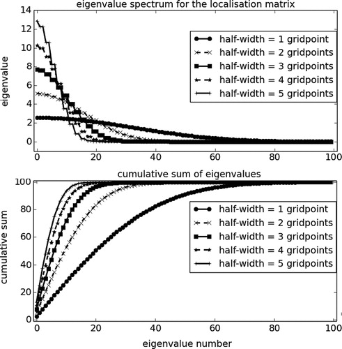
Let us illustrate this in Fig. 8 with an example. For a system with grid points, we generate localisation matrices using different half-widths (shown with different line styles in the figure), and we perform their spectral decompositions. The top panel shows the eigenvalues, in decreasing order of magnitude, for each one of the different half-widths. The decay in magnitude is slow for , but it becomes considerably faster as the half-width increases. The bottom panel shows the cumulative sum of these eigenvalues. For it quickly approaches its maximum value , and many eigenvalues contribute to this sum only marginally, especially for larger localisation half-widths.

Fig. 8. Eigenvalue spectrum of a localisation matrix for grid points, with different localisation half-widths (different lines). The top panel shows the eigenvalues in descending order, while the bottom panel shows their cumulative sum.

Small eigenvalues can be discarded in favour of speeding up the computation time, creating a simpler minimisation problem. The minimisation becomes easier for two reasons. First the size of the control vector decreases. Second, considering small grid point-per-grid point variations (a consequence of keeping all eigenvalues) can result in a more difficult minimisation problem.

To determine the number of eigenvalues to keep, a simple idea is to chose the value that fulfils:

(58)

where the eigenvalues are ordered by decreasing magnitude, and is a fraction of our choice. The closer to one this fraction is, the closer our cropped localisation matrix will be to the original one. The in the right hand side of (58) comes from the fact that .

In Fig. 9 we have illustrated this choice for two fractions: in the left panel and in the right panel. For different total number of grid points (lines with different colors), we show the ratio required as a function of the localisation radius (half-width of the Gaspari Cohn function). As expected this normalized quantity depends only on the localisation radius, and it is a decreasing function. This corresponds perfectly with our previous discussion of the two limiting cases.

Fig. 9. Construction of in SC and WC4DEnVar. For different number of grid points and different localisation half widths (horizontal axis), the vertical axis shows the ratio of retained eigenvalues over , in order to cover a given fraction of the total sum of eigenvalues. For the left panel this fraction is , in the right panel it is .

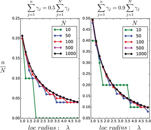
An example of the reduction in computational cost can be seen, for example, at . If our desired fraction is , we would need to keep around of the total number of eigenvalues. If our desired fraction were the required fraction would be reduced to .

Appendix 2. Generating

The method used in Yang et al. (2006) is is outlined next. The purpose is to create a climatological background error covariance matrix in an iterative manner.

1. The process starts by proposing a guess matrix . This can be as simple as the identity matrix. However, we start with a circulant matrix, with the row being .

2. We perform a 3DVar assimilation experiment using observations every 5 model time steps, with all grid points observed being observed. This is done for assimilation cycles, and we use the proposed .

3. At this point we have 100 forecast values (valid at the assimilation instants) which can be compared to the nature run. We use these values to find a full-rank sample estimator .

4. We replace our previous value of with the one just computed from sample statistics and repeat steps 2 and 3; we perform 10 iterations (in fact, we found convergence after 5).

5. We repeat the whole procedure 20 times, each with a different set of pseudo-observations. We average the 20 estimators and that yields the final estimator of .

References

- Bannister, R. N. 2008. A review of forecast error covariance statistics in atmospheric variational data assimilation. II: Modelling the forecast error covariance statistics. Q.J.R. Meteorol. Soc. 134, 1971–1996. DOI:10.1002/qj.v134:637.
- Bishop, C., Etherton, B. and Majumdar, S. 2001. Adaptive sampling with the ensemble transform Kalman filter. Part I: Theoretical aspects. Mon. Weather Rev. 129, 420–436. DOI:10.1175/1520-0493(2001)129<0420:ASWTET>2.0.CO;2.
- Bloom, S., Takacs, L., DaSilva, A. and Ledvina, D. 1996. Data assimilation using incremental analysis updates. Mon. Wea. Rev. 124(6), 1256–1271. DOI:10.1175/1520-0493(1996)124<1256:DAUIAU>2.0.CO;2.
- Bonavita, M., Isaksen, L. and Holm, E. 2012. On the use of EDA background error variances in the ECMWF 4D-Var. Q. J. R. Meteorol. Soc. 138, 1540–1559. DOI:10.1002/qj.1899.
- Buehner, M. 2005. Ensemble-derived stationary and flow- dependent background error covariances: Evaluation in a quasi-operational NWP setting. Q. J. R. MeteoR. Soc. 131, 1013–1043. DOI:10.1256/qj.04.15.
- Clayton, A. M., Lorenc, A. C. and Barker, D. M. 2013. Operational Implementation of a Hybrid Ensemble/4D-Var Global Data Assimilation System at the Met Office. Quart. J. Roy. Meteor. Soc. DOI:10.1002/qj.2054.
- Evensen, G. and Van Leeuwen, P. J. 2000. An ensemble Kalman smoother for nonlinear dynamics. Mon. Wea. Rev. 128, 1852–1867. DOI:10.1175/1520-0493(2000)128<1852:AEKSFN>2.0.CO;2.
- Fairbarn, D., Pring, S., Lorenc, A. and Roulsone, I. 2014. A comparison of 4DVAR with ensemble data assimilation methods. Q.J.R. Meteorol. Soc. 140, 281–294. DOI:10.1002/qj.2135.
- Gaspari, G. and Cohn, S. E. 1999. Construction of correlation functions in two and three dimensions. Q. J. R. Meteorol. Soc. 125, 723–757. DOI:10.1002/qj.49712555417.
- Goodliff, M., Amezcua, J. and Van Leeuwen, P. J. 2015. Comparing hybrid data assimilation methods on the Lorenz 1963 model with increasing non-linearity. Tellus A 67, 26928. DOI:10.3402/tellusa.v67.26928.
- Hunt, B. R., Kostelich, E. J. and Szunyogh, I. 2007. Efficient data assimilation for spatiotemporal chaos: a local ensemble transform Kalman filter. Phys. D 230, 112–126. DOI:10.1016/j.physd.2006.11.008.
- Kalnay, E. and Yang, S.-C. 2010. Accelerating the spin-up of Ensemble Kalman Filtering. Quart. J. Roy. Meteor. Soc. 136, 1644–1651. DOI:10.1002/qj.652.
- Lawson, W. G. and Hansen, J. A. 2005. Alignment Error Models and Ensemble-Based Data Assimilation. Mon. Wea. Rev. 133, 1687–1709. DOI:10.1175/MWR2945.1.
- Le Dimet, F.-X. and Talagrand, O. 1986. Variational algorithms for analysis and assimilation of meteorological observations: theoretical aspects. Q. J. R. Meteorol. Soc. 38A, 97–110.
- Liu, C., Xiao, Q. and Wang, B. 2008. An ensemble-based four-dimensional variational data assimilation scheme. Part I: Technical formulation and preliminary test. Mon. Wea. Rev. 136(9), 3363–3373. DOI:10.1175/2008MWR2312.1.
- Lorenc, A. 2003. The potential of the ensemble Kalman filter for NWP – a comparison with 4D-Var. Q. J Roy. Meteorol. Soc. 129(595B), 3183–3203. DOI:10.1256/qj.02.132.
- Lorenc, A. C., Bowler, N. E., Clayton, A. M., Pring, S. R., and Fairbairn, D. 2015. Comparison of hybrid-4DEnVar and hybrid-4DVar data assimilation methods for global NWP. Q J. Roy. Met. Soc. 143. DOI:10.1175/MWR-D-14-00195.1.
- Lorenz, E. 1963. Deterministic Non-periodic Flow. J. Atmos. Sci. 20, 130–141.
- Lorenz, E. N. 1996. Predictability: A problem partly solved. In: Proc. ECMWF Seminar on Predictability, 4–8 September 1995, Reading, UK, pp. 1–18.
- Lorenz, E. N. 2005. Designing chaotic models. J. Atmos. Sci. 62, 1574–1587. DOI:10.1175/JAS3430.1.
- Miyoshi, T. 2011. The Gaussian approach to adaptive covariance inflation and its implementation with the local ensemble transform Kalman filter. Mon. Weather Rev. 139, 1519–1535.
- Parrish, D. F. and Derber, J. C. 1981. The National Meteorological Center’s spectral statistical interpolation analysis system. Mon. Weather Rev. 120, 1747–1763. DOI:10.1175/1520-0493(1992)120<1747:TNMCSS>2.0.CO;2.
- Shu, -J.-J. 1987. The proper analytical solution of the Korteweg-de Vries-Burgers equation. J. Phys. A Math. Gen. 20(2), 49–56. DOI:10.1088/0305-4470/20/2/002.
- Simon, D. 2006. Optimal State Estimation. John Wiley & Sons, New York, 552 p.
- Talagrand, O. and Courtier, P. 1987. Variational Assimilation of Meteorological Observations With the Adjoint Vorticity Equation. I: Theory. Q.J.R. Meteorol. Soc. 113, 1311–1328. DOI:10.1002/qj.49711347812.
- Tremolet, Y. 2006. Accounting for an imperfect model in 4D-Var. Q. J. R. Meteorol. Soc. 132, 2483–2504. DOI:10.1256/qj.05.224.
- Van Leeuwen, P. J. 2003. A Variance-Minimizing Filter for Large-Scale Applications. Mon. Wea. Rev. 131, 2071–2084. DOI:10.1175/1520-0493(2003)131<2071:AVFFLA>2.0.CO;2.
- Van Leeuwen, P. J. and Evensen, G. 1996. Data assimilation and inverse methods in terms of a probabilistic formulation. Mon. Wea. Rev. 124, 2898–2914. DOI:10.1175/1520-0493(1996)124<2898:DAAIMI>2.0.CO;2.
- Wang, X., Bishop, C. and Julier, S. 2004. Which is better, an ensemble of positive-negative pairs or a centered spherical simplex ensemble?. Mon. Wea. Rev. 132, 1590–1605. DOI:10.1175/1520-0493(2004)132<1590:WIBAEO>2.0.CO;2.
- Wang, X., Snyder, C. and Hamill, T. M. 2007. On the Theoretical Equivalence of Differently Proposed Ensemble 3DVAR Hybrid Analysis Schemes. Mon. Wea. Rev. 135, 222–227. DOI:10.1175/MWR3282.1.
- Whitaker, J. S. and Hamill, T. M. 2002. Ensemble data assimilation without perturbed observations. Mon. Weather Rev. 130, 1913–1927. DOI:10.1175/1520-0493(2002)130<1913:EDAWPO>2.0.CO;2.
- Wursch, M. and Craig, G. C. 2014. A simple dynamical model of cumulus convection for data assimilation research. Meteorologische Zeitschrift 23(5), 483–490.
- Yang, S.-C., Baker, D., Li, H., Cordes, K., Huff, M.et al. 2006. Data assimilation as synchronization of truth and model: experiments with the three-variable Lorenz system. J. Atmos. Sci. 63(9), 2340–2354. DOI:10.1175/JAS3739.1.
- Zakharov, V. E. and Faddeev, L. D. 1971. Korteweg-de Vries equation: A completely integrable Hamiltonian system. Funct. Anal. Appl. 5(4), 280–287. DOI:10.1007/BF01086739.
- Zupanski, M. 2005. Maximum likelihood ensemble filter: theoretical aspects. Mon. Wea. Rev. 133(6), 171–1726. DOI:10.1175/MWR2946.1.