A weak-constraint 4DEnsembleVar. Part II: experiments with larger models

ABSTRACT

In recent years, hybrid data-assimilation methods which avoid computation of tangent linear and adjoint models by using ensemble 4-dimensional cross-time covariances have become a popular topic in Numerical Weather Prediction. 4DEnsembleVar is one such method. In spite of its capabilities, its application can sometimes become problematic due to the not-trivial task of localising cross-time covariances. In this work we propose a formulation that helps to alleviate such issues by exploiting the presence of model error, i.e. a weak-constraint 4DEnsembleVar. We compare the weak-constraint 4DEnsembleVar to that of other data-assimilation methods. This is part II of a two-part paper. In part I, we describe the 4DEnsembleVar framework and problems with localised temporal cross-covariances associated with this method are discussed and illustrated on the Korteweg de Vries model. We also introduce our weak-constraint 4DEnsemble-Var formulation and show how it can alleviate—at least partially—the problem of having low-quality time cross-covariances. The second part of this paper deals with experiments on larger and more complicated models, namely the Lorenz 1996 model and a modified shallow-water model with simulated convection, both of them under the presence of model error. We investigate the performance of weak-constraint 4DEnsembleVar against strong-constraint 4DEnsembleVar (both with and without localisation) and other traditional methods (4DVar and the Local Ensemble Transform Kalman Smoother). Using the analysis root mean square error (RMSE) as a metric, these methods have been compared considering observation density (in time and space), observation period, ensemble sizes and assimilation window length. In this part we also explain how to perform outer loops in the EnVar methods. We show that their use can be counter-productive if the presence of model error is ignored by the assimilation method. We show that the addition of a weak-constraint generally improves the RMSE of 4DEnVar in cases where model error has time to develop, especially in cases with long assimilation windows and infrequent observations. We have assumed good knowledge of the statistics of this model error.

Keywords:

• data assimilation
• hybrid methods
• convective data assimilation

1. Introduction

This is the second part of a study to introduce a new hybrid ensemble-variational (EnVar) data assimilation (DA) method, which takes into consideration the presence of model error. We have denominated this method a weak-constrained 4DEnsembleVar (WC4DEnVar).

In part I of this work we provided a review of the 4DEnVar framework in the strong-constraint (SC) case. We paid particular emphasis on the localisation process and we illustrated the problems associated with localising 4-dimensional time cross-covariances using static localisation matrices, especially when the assimilation window is long.

We then proposed making use of additive model error and implement localised 4DEnVar in the weak-constraint (WC) framework. In particular, we based our method in the model-bias correction formulation of WC4DVar—see Tremolet (2006)—and we provided a discussion on the rationale behind our choice of control variable. We showed that our method distributes the analysis increments over more time instants in the assimilation window (other than the initial time), and hence it alleviates—at least partially—the problems generated by wrongly localised time cross-covariances. For this purpose we used the Korteweg de Vries (KdV) model for the perfect evolution of a coherent structure (a soliton).

In the present paper (part 2) we study the behaviour of this promising DA method in more elaborated settings. First we experiment on a stochastic implementation of the N_x-variable Lorenz 1996 (L96) model (Lorenz, 1996, 2005). In this model we can explore the use of localisation with a range of small ensemble sizes. The moderate size of the model also allows us to perform detailed studies on a combination of parameters such as localisation radii, observational frequency in time, observational density in space, number of observations per assimilation window, and the use of outer loops in the minimisation procedure for the EnVar methods. As with this model, we have both the tangent linear and adjoint models (TLM and AM, respectively), we can do comparisons to SC4DVar and WC4DVar.

The second model we use is a one-dimensional modified shallow-water equation (SWE) model developed by Wursch and Craig (2014) which simulates convection, and can be implemented stochastically. This accessible and relatively inexpensive model has recently been used as a test-bed for convective-scale DA (Perianez et al., 2014). This model provides a challenging environment for experimentation. For instance, its three variables (velocity, height and rain) possess considerably different time and length scales. Rain is a non-negative–definite variable with a non-Gaussian distribution which presents challenges to conventional DA methods. We do not compare with 4DVar (either SC or WC) because we do not have the TLM or AM in this case.

This paper is organized as follows. Section 2 gives a brief description of the use of outer loops for WC4DEnVar, and the differences with respect to their implementation in the variational framework. Section 3 contains the experiments with the L96 model. Section 4 describes the modified SWE and shows the results of our experiments with this model. Section 5 provides a summary of our work and main results. Section 6 concludes the work and gives ideas for future avenues of research. In this paper we use notation that has already been defined in part I. Only new symbols are defined explicitly. Any time we mention the WC formulation (either in the 4DVar or 4DEnVar context), we refer the model-bias correction version.

2. Outer loops in WC4DEnVar

We explore the use and performance of outer loops in the hybrid EnVar schemes. For a detailed discussion on inner and outer loops, the reader is referred to Tremolet (2004).

To implement outer loops in WC4DEnVar, the control variables in our preconditioned incremental minimisation problem are:

(1)

where the superscript g stands for guess, and we have used and . With these control variables, we can write the gradient as the following vector:

(2)

where d^t are now computed as:

(3)

For the ‘zeroth’ outer loop, we have and . For all subsequent outer loops the ‘guess’ values are equal to the analysis values obtained in the previous outer loop.

For variational methods, in every outer loop the TLMs and AMs are re-computed, because the reference trajectory has been updated. This means that for the EnVar methods the covariances and have to be recomputed, which requires re-running the free ensemble from the new guess for both initial conditions and model error innovations. In practice, this can be very costly and sometimes infeasible. For this reason, in the EnVar methods these covariances are fixed through all outer loops.

The implementation of outer loops in the SC case is similar to the process outlined; the only difference is that the model error terms are not included.

3. Experiments with Lorenz 96

In this section we evaluate in detail the performance of WC4DEnVar and compare it to the performance of other DA methods, in particular that of SC4DEnVar (with and without localisation). We choose the widely known L96 model with N_x grid points. This non-linear and chaotic system is described by the solution of the following set of ordinary differential equations (ODEs):

(4)

for n = 1 … N_x. The indices are modular, i.e. . The first term on the right-hand side of eq. (4) represents non-linear advection, the second term represents damping, and the third term represents forcing, with F = 8. In particular we use N_x = 24 grid points, a size that requires localisation and that allows us to perform long-enough experiments (to get robust statistics) and to explore the impact of different parameters in the DA methods.

To make this model imperfect we implement the following map:

(5)

where represents the deterministic solution of eq, (4) using a 4th-order Runge–Kutta method over a time step Δt = 0.01—Lorenc et al. (2015) recommends Δt ≤ 0.025 for the perfect-model case—and represents the model error contribution. For the model error covariance matrix Q we use a circulant matrix whose jth row is:

(6)

where we choose . This is the model error variance within a Δt = 0.01 time step (i.e. this number is already scaled by Δt).

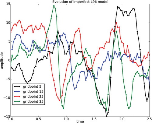
We perform identical twin experiments. To generate the true run we initialise the model by starting from an initial condition selected as a random perturbation of the (unstable) fixed point of the system, with perturbations coming from a rv N(0,I). The model is run for 200 time steps to eliminate any transient, and this is the initial condition for the true run, which we label x^0,truth. This nature run consists of 700 time steps. In Fig. 1 we show the time evolution for the variables—represented with different colours—in the interval 0 ≤ t ≤ 5.

Fig 1. Time evolution of the nature run for the imperfect L96 model in the interval 0 ≤ t ≤. We choose four grid points which we depict in different colours.

It is important to quantify the variability inherent to our model. We do this by evolving two trajectories: the true trajectory in the interval 0 ≤ t ≤ 200 and a perturbed trajectory started from a nearby initial condition. Then we compute the RMSE (root mean squared error) for every time step as:

(7)

The climatological saturation error is computed as the time mean of this time-dependent RMSE, yielding a value of

(8)

where the value in parentheses indicates the standard deviation over all time steps.

After defining the truth, synthetic observations are generated by perturbing the true run every time step with a random variable , where . That is, the observational error is spatially uncorrelated and has a standard deviation . For our experiments, we take subsets of them, both in space and time.

We also generate a climatological error covariance B^c, which we will need in our DA experiments. We construct this matrix following the method of Yang et al. (2006). A brief description of this method is described in Appendix B of the first part of this paper. To create this matrix we use observations in all grid points, and every two model steps. The B^c obtained was post-processed by averaging each off-diagonal in the matrix. This assumes that the background error covariance between two grid points only depends on the distance between them. The resulting B^c is a circulant matrix, for which the value for the jth row are:

(9)

3.1. First experiments

3.1.1. A densely covered grid

We need to make sure that all of our DA methods are working, especially the ones we have proposed in part I of this paper. Hence, our first experiment has very simple settings: observations at every single grid point and every time step. The results of this experiment are shown in Fig. 2.

Fig 2. DA experiments in the L96 imperfect model with observations every time step and at every grid point. The left panel shows the true trajectory of variable x⁽²⁾ (grey line), as well as the observations (grey dots). The coloured lines show the analysis trajectories by different DA methods (see legend). The middle panel shows the time evolution of the analysis RMSE. The right panel shows non-parametric statistics (25 percentile, median and 75 percentile) computed over time for each method.

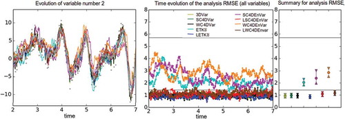
We compare the following DA methods: 3DVar, SC4DVar and WC4DVar, ETKS and LETKS, SC4DEnVar and WC4DEnVar, LSC4DEnVar and LWC4DEnVar. The ensemble and hybrid methods use adaptive inflation (Miyoshi 2011). To emulate real situations where ensemble sizes are limited, for the ensemble and hybrid methods we use an ensemble size N_e = 4. The localised versions of these methods use λ = 2. For the variational and hybrid methods we use 0 outer loops, and there is only one observational time in an assimilation window. In the hybrid methods we use 11 eigenvalues for (similar results were obtained with {9,13,15}, which we do not show for brevity).

Figure 2 has three panels. The left panel shows the time evolution of x⁽²⁾. The true evolution is shown in grey, and the grey dots correspond to the observations. The coloured lines show the analysis trajectories obtained by the different DA methods: see the legend for correspondence. The middle panel shows the time evolution of the analysis RMSE computed over all grid points. There are two horizontal grey lines; the lower one corresponds to the observational error standard deviation, while the upper one corresponds to the climatological RMSE computed earlier. In the right panel we show summary statistics (over time) for the analysis RMSE. In particular, we show an interval formed of the 25% percentile (upper triangle), median (circle) and 75% percentile (lower triangle). We eliminate the first 200 model steps as a transient and compute the statistics over the last 500 model steps only.

In this ‘easy’ setup most of the methods perform well, with RMSEs well under the observational error level. The performance of the three variational methods is practically indistinguishable. For the ensemble and hybrid methods, the effect of having a small sample size shows up in all of the non-localised methods. The RMSE of ETKS, SC4DEnVar and WC4DEnVar is larger than the observational error level. These RMSE values show large variations in their time evolution. It is important to note that the RMSE of WC4DEnVar is considerably larger than that of ETKS, which is understandable because the same small ensemble size—and hence noisy covariance information—is being used to update variables at two time steps. As expected, any problems coming from small sample sizes are immediately fixed with the introduction of localisation. The RMSEs for LETKS, LSC4DEnVar and LWC4DEnVar are below observational level, with LETKS performing the best. The time evolution of the RMSE in these localised methods is quite steady, the jumps that occurred without localisation are not present.

3.1.2. The land–sea configuration

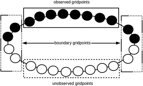
Let us move to a more challenging situation. We use the configuration shown in Fig. 3. This is the so-called land–sea configuration in which half of the grid points are observed (black grid points) and half of the grid points are not observed (white grid points). For our analysis we divide the grid into three sets: the eight central observed grid points are denominated ‘observed grid points’, the eight central unobserved grid points are denominated ‘unobserved grid points’ and the four grid points (two observed and two unobserved) in each one of the two boundaries (i.e. eight grid points in total) are denominated ‘boundary grid points’. We do this separation considering that the behaviour of the RMSE in each of these sets will be different. In the (central) unobserved grid points the analysis trajectories are closer to a free run. The boundary grid points, on the other hand, do feel the impact of observations. If the information communicated has high quality, the analysis should be close to the truth. If the information is poor, the trajectories will be off the truth and will not be smooth (which is different from free runs). We choose the number of boundary grid points considering that the decorrelation length scale of the system is about 1 grid point.

Fig 3. Land sea configuration used for our DA experiments. Twelve variables are observed and 12 are unobserved. We divide the grid into three types of variables: observed, unobserved and boundary variables.

We perform experiments with two observational frequencies: 1 model step. We keep the same settings as in the previous case: no outer loops, N_e = 4, λ = 2, and one observational time per assimilation window. We eliminate the first 200 model steps of the experiment as a transient and compute statistics for 2 ≤ t ≤ 7.

The results of these experiments are shown in Fig. 4 (observational period of 1) and Fig. 5 (observational period of 2). Each figure has three rows and two columns. The top row shows results for the observed grid points, the middle row for the unobserved grid points and the bottom row for the boundary grid points. The left column shows the time evolution for the RMSE of the analysis trajectory obtained by each DA method (different colours), while the right column shows the non-parametric summary statistics.

Fig 4. Analysis RMSE results for the imperfect L96 model under the land–sea configuration with observations every model step. We show the time evolution (left columns) and the summary statistics (right columns) for the different variables (rows). Different coloured lines correspond to different methods (see legend).

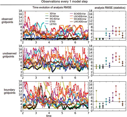
Fig 5. Same as Fig. 4, but with observations every two model steps.

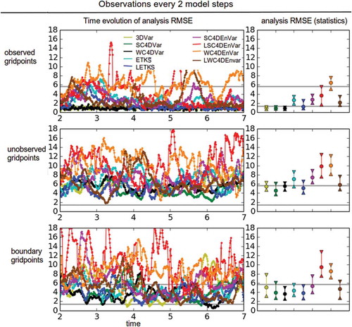
This spatial configuration leads to large differences in the performance of the methods. For the observed variables, 3DVar, SC4DVar and WC4DVar perform similarly well, and the time evolution of the analysis RMSE is steady. ETKS does not perform well without localisation, but this is obviously improved by LETKS. We did not optimise the localisation half-width, which explains why the RMSE does not reach to the levels of the variational methods. The best of the hybrid methods is LWC4DEnVar. The other three methods have RMSEs close to the climatological error, and localisation does not seem to help SC4DEnVar. In fact, LSC4DEnVar performs worse in the case of observations every two steps.

For the unobserved grid points, the RMSE of the three variational methods, LETKS and LWC4DEnVar are close to the climatological error. The time evolution of the analysis RMSE of these methods is not as smooth as for the observed variables. The RMSE values of non-localised methods—ETKS, SC4DEnVar and WC4DEnVar—are above the climatological level. This is understandable since our small sample size (N_e = 4) can introduce spurious long-term correlations and lead to incorrect innovations in the unobserved region. This is not undone by localisation in the case of LSC4DEnVar. The time evolution of the RMSE of these methods is volatile.

In the boundary grid points we observe the largest variability in the time evolution of the analysis RMSE for all methods. For variational methods, the intervals shown for the summary statistics are large, especially for 3DVar. ETKS and LETKS perform similarly (again, this may be improved by optimising λ). The RMSE values for SC4DEnVar and WC4DEnVar are larger than the climatological error, as was the case for unobserved variables. For boundary variables, localisation clearly acts in different ways for these methods. LSC4DEnVar has the largest RMSE of all methods, while LWC4DEnVar has a RMSE value comparable to that of the variational methods. For both observational frequencies localisation seems to be bad for SC4DEnVar. Even with observations every two steps, it seems like a short time for advection to interfere with static localisation. This result can be a combination of the small sample size, a badly tuned localisation radius, and variability in the performance of the methods for boundary grid points. For this reason, we perform a much more detailed parameter exploration in the following subsection.

3.2. Exploring parameters

In the previous experiments we gave particular values to different parameters of the DA methods. Let us fix the observational grid as the one land-sea configuration and the observation frequency at two model steps. We explore the sensitivity to all other parameters. For this purpose we present a series of ‘mosaic plots’, i.e. two-dimensional plots in which the values of two parameters are varied simultaneously, and we display the RMSE value of every corresponding combination. Note that the variation in the colour scheme is not linear. We give extra resolution to the values 0.2 ≤ RMSE ≤ 2 (recall that ), and less resolution for 2 < RMSE ≤ 7 Anything corresponding to RMSE > 7 is plotted in white, and is considered an unsuccessful experiment. We choose this value based on the mean climatological RMSE (and its standard deviation) computed before. We run the DA methods for 1200 model steps and eliminate the first 200 time steps as a transient. We then compute the RMSE of the analysis trajectories for the remaining 1000 time steps, and present the median in the plot. We do this separately for observed (left panels in all plots), unobserved (middle panels in all plots) and boundary grid points (right panels in all plots).

3.2.1. Ensemble methods

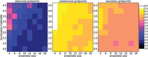
First we take a look at the performance of LETKS. The results of this experiment are presented in Fig. 6. For each panel, the horizontal axis indicates different ensemble sizes: N_e = {4,6,8,10,12,14,16,18}, while the vertical axis corresponds to different localisation half-widths: λ= {0.5,1.1.5,2,2.5,3,3.5,4,4.5}. The results of these experiments confirm our intuition: small ensemble sizes require quite strict localisation to eliminate spurious information, while larger ensemble sizes contain less noisy information and hence perform well in a large range of localisation values. As expected, the largest RMSE values are those of the unobserved grid points, the second largest values are those of the boundary points, and then lowest values correspond to the observed grid points. For really small ensemble sizes, strict localisation half-widths λ ≤ 2.0 are required to ensure a successful DA process.

Fig 6. Median analysis RMSE over 1000 time steps for LETKS with the imperfect L96 with land–sea configuration and observations every two time steps. Different ensemble sizes (horizontal axis) and different localisation half-widths (vertical axis) are tested. Each panel represents a different kind of variable.

3.2.2. Variational methods

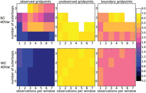
Let us move to the experiments using variational DA methods. The results of these experiments are shown in Fig. 7, with the top row corresponding to SC4DVar and the bottom row corresponding to WC4DVar. The horizontal axis corresponds to the number of observational times in each assimilation window (labelled opw, observations per window): opw = {1,2,3,4,5,6,7} (which changes the size of the assimilation window), and the vertical axis corresponds to the number of outer loops. For SC4DVar with no outer loops, it seems that the optimal number of observational times in an assimilation window is 3 to 7. We especially observe this in the case of the observed variables. Interestingly, as we introduce outer loops the quality of the analysis decreases drastically (except for the case with only one observational time and one outer loop). This is true for observed, unobserved and boundary variables. In fact, for the case of unobserved variables the outer loops take all value from the assimilation (RMSE > 7). This is not the same in the WC4DVar case, where we observe that the assimilation is pretty robust to the number of outer loops. For WC4DVar, longer assimilation windows are favoured. In fact, the best results occur with more than three observational times per assimilation window. For WC4DVar the RMSE values for observed variables are consistently under the observational error level, the RMSE values of unobserved variables are constantly around the climatological level, and the RMSE values for the boundary variables are always in between. These results suggest that the re-centring process of the outer loops can be damaging when using a SC4DVar in the presence of moderate model error. More experimentation on this regard is needed, but it is beyond the scope of this work.

Fig 7. Median analysis RMSE over 1000 time steps for variational methods with the imperfect L96 with land–sea configuration and observations every two time steps. The top row shows results for SC4DEnVar, while the bottom row shows results for WC4DEnVar. Different numbers of observational times per analysis window (horizontal axis) and numbers of outer loops (vertical axis) are tested.

3.2.3. Non-localised EnVar methods

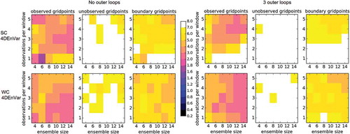
Let us move on to the EnVar methods; first we take a look at these methods with no localisation. We show the results of these experiments in Fig. 8. The figure has two sides: the left side corresponds to no outer loops, while the right side corresponds to three outer loops. As usual the top row corresponds to SC4DEnVar and the bottom row to WC4DEnVar. The horizontal axis in each mosaic plot corresponds to the ensemble size N_e = {4,6,8,10,12,14}, while the vertical axis corresponds to the number of observational times within the assimilation window: opw = {1,2,3,4,5} (this changes the size of the assimilation window). We first look at the observed variables. The RMSE value rarely goes below observational level regardless of the ensemble size (at least for the sizes studied). When outer loops are introduced, the performance of SC4DEnVar is damaged, while that of WC4DEnVar improves (see the right top corner of the corresponding panel). For unobserved variables, in both SC and WC4DEnVar difficulties are encountered, with usual cases of RMSE > 7. We speculate that long-range spurious correlations lead to fictitious increments that damage the assimilation. The number of ‘successful’ DA cases, however, is slightly larger for the WC4DEnVar case. The presence of outer loops damages the assimilation considerably in the two cases. For the boundary variables and no outer loops the RMSE value of WC4DEnVar is close to climatology, whereas for SC4DEnVar there are cases with RMSE > 7. This is understandable considering the spurious information coming from such noisy sample estimator for the 4D covariance matrices. The presence of outer loops considerably damages the performance of SC4DEnVar. The presence of outer loops in WC4DEnVar damaged (slightly) the performance of the method, but it only led to a failed DA experiment in one combination of parameters.

Fig 8. Median analysis RMSE over 1000 time steps non-localised EnVar methods (top row for SC4DEnVar, bottom row for WC4DEnVar) with the imperfect L96 with land–sea configuration and observations every two time steps. No outer loops (left half) and three outer loops (right half) are used. For each panel, we vary the ensemble size (horizontal axis) and the number of observations per window (vertical axis).

3.2.4. Localised EnVar methods

Finally, let us perform a last set of experiments addressing the performance of LSC4DEnVar and LWC4DEnVar. The results of these experiments are depicted in Fig. 9. The top half of the figure corresponds to the results with no outer loops, while the bottom half corresponds to the results with three outer loops. As usual, there are two rows (top for LSC4DEnVar, bottom for WC4DEnVar) and three columns (each for a different type of grid point). In each panel we have stacked three mosaic plots on top of each other. Each corresponds to a different ensemble size, increasing vertically. We have focused in small ensemble sizes: N_e = {4,6,8}, which are challenging for these methods. The two horizontal axes of each panel correspond to observations per window opw = {1,2,3,4,5} (which change the length of the assimilation window) and localisation half-width λ = {1,1.5,2,2.5,3,3.5,4,4.5}.

Fig 9. Median analysis RMSE over 1000 time steps EnVar methods (top rows for LSC4DEnVar, bottom rows for LWC4DEnVar) with the imperfect L96 with land–sea configuration and observations every two time steps. No outer loops (top half) and three outer loops (bottom half) are used. Different columns show different variables (left for observed, middle for unobserved and right for boundary variables). In each panel we show the variation with respect to three parameters: observations per window and localisation half-width in the horizontal axes, and ensemble size in the vertical axis.

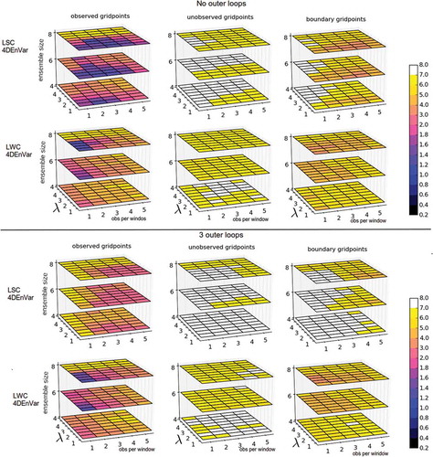
Let us start with the case of no outer loops. As the ensemble size increases the performance of the methods improves, and this is true for the three types of variables. In the case of observed variables LSC4DEnVar performs slightly better than LWC4DEnVar, although it is important to notice that the best results are for LWC4DEnVAr in the case of one observation per window and λ = 1.0. For LSC4DEnVar, larger localisation half-widths allow for more observational times per window (up to a point). Notice that the case of two observations per window allows for the biggest range of localisation half-widths. For the unobserved grid points we notice that LSC4DEnVar struggles to keep the RMSE within the climatological level, with many white cases (RMSE > 7). LWC4DEnVar is more robust, because only the case M = 4 struggles. This is also true for the boundary grid points; in this case, LWC4DEnVar is successful for all configurations, while LSC4DEnVar struggles in some cases (this reduces as the ensemble size grows). The introduction of outer loops degrades the performance of the DA methods in both cases, but it is much more damaging for the LSC4DEnVar case. This coincides with the fact that outer loops were not beneficial with SC4DVar in the presence of model error which is ignored by the assimilation system.

In the 4DVar cases, the outer loops damaged the SC (when the minimisation ignored the presence of model error), but not the WC (when the minimisation included the model error, albeit in a simplified manner). In the EnVar case, outer loops damage the results for both LSC and LWC cases, although the problem is considerably worse for LSC. There have been studies on convergence of outer loops in 4DVar (e.g. Tremolet, 2007), which have shown that over-solving the inner loop minimisation can trap the incremental algorithm away from the true minimum by fitting observational noise and introducing spurious gradients. We think that in our case spurious gradients may be introduced by the localisation, but a more detailed study is needed before stating conclusions.

4. Experiments on the shallow-water model

In this section we discuss the implementation and working of WC4DEnVar in a non-linear SWE model which includes equations that mimic the formation of convective cumulus clouds and rain. The model by Wursch and Craig (2014) was developed to give a computationally friendly model which is inexpensive to run but physically plausible. The model is based on the SWEs:

(10)

(11)

where eq. (10) is the momentum equation and eq. (11) is the continuity equation. Here, u is the fluid velocity, H is the thickness of the undisturbed layer (without waves), h now represents the deviation from that level due to the wave motion, K is the diffusion coefficient and is the geopotential. This SWE model can be run with or without model error. The right-hand side of eqs (10) and (11) parametrises the subgrid processes, which cannot be modelled directly.

In nature, convective clouds are caused by boundary layer air rising due to disturbances, causing it to reach a level of free convection. In our experiments, we are triggering convective cloud through the wave motion when the layer height becomes larger than H_c. The SWEs are modified to represent cumulus cloud convection and rain as follows:

(12)

where

(13)

in which r represents the rain variable. To create convective updraft, a forcing term F has been added to the model eq. (12). The evolution equation for rain is:

(14)

where is a constant geopotential corresponding to the chosen H_c, which is the height at which clouds are formed. In the modified momentum equation, momentum is adjusted by gradients in the rain rate mimicking the influence of down drafts due to the rain. When Z > H_r the momentum gradient couples back to the rain rate proportional to β representing the influence of updrafts on rain intensity. H_r > H_c to delay rain formation by about 15 minutes, and leading to a cloud life time of 1–2 hours. Finally, the term proportional to α provides a simple Newtonian damping of the rain intensity.

The parameters in these equations are chosen such that the system evolution appears chaotic, with values H_c = 90.02m, H_r = 90.4m, β = 1/300, α = 2.5 × 10^–4 s^–1, , K = 8000, K_r = 0.15K.

For our numerical implementation, we write the equations in conservative form. The model is discretised in space using a second-order central difference scheme except for the diffusion terms. For these, we use upwind differences. In time, we use

(15)

where is a map which evolves the model from t to I + 1 by using the 4th-order Runge–Kutta method over one time step (with Δt = 0.025). The model error n is a random vector chosen from a Gaussian distribution such that n: N(0,Q) where Q is the covariance matrix for one time step. This method is known as the hybrid Runge–Kutta 4th-order method and is given in Hansen and Penland (2006).

The horizontal distance between grid points is dx = 500m and the time step length is dt = 40s. Hovmuller plots of the model trajectories are shown in Fig. 10.

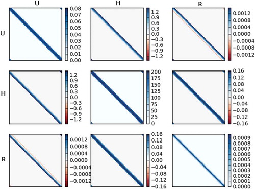
4.1. Generation of the error covariance matrices

The climatological background error covariance matrix was generated using the method of Yang et al. (2006) and described in Appendix 2 of the first part of this paper. We applied localisation to eliminate round-off error and spurious correlations.

To smooth this matrix, we used a Schur product such that

(16)

where is our localised background error covariance matrix and L_xx is our localisation matrix, which in this case is created using a step function with length of five grid points. The resulting matrix is shown in Fig. 11.

Fig 10. Hovmuller plots for the SWE model (with model error) showing the evolution of the truth. Each plot shows the time steps on the y-axis and the grid point number on the x-axis. The colour bars show the velocity, the height and the rain, respectively.

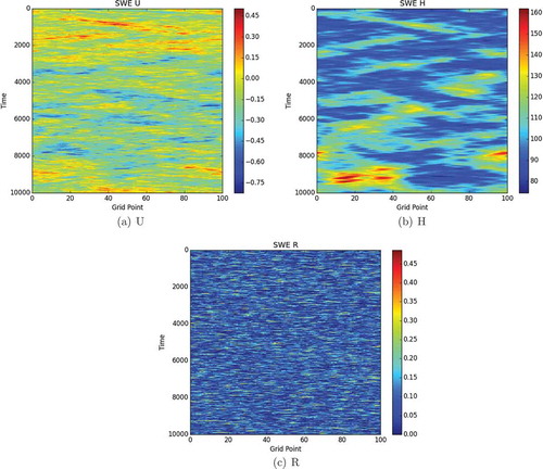
Fig 11. Climatological B matrix for the SWE model (with model error) over 100 grid points. See text for the description of its generation. Each panel shows the covariances between variables of the correspoding row and column in the figure.

The observation error covariance matrix is given as

with where , . Also, we assume that all observations are uncorrelated.

The model error covariance matrix is given as

with where , , and is a circulant matrix with the first row [1, 0.5, 0.25, 0, … 0, 0.25, 0.5]. The purpose of this choice is to allow small-scale communication among neighbouring grid points, representing missing model physics due to sub-grid-scale processes. We also did experiments where , , as comparison. The results found were similar to the ones in this paper and will not be shown.

4.2. Experiments and results

In this section, we present a comparison between SC4DEnVar, LSC4DEnVar, WC4DEnVar and LWC4DEnVar. For large non-linear models, 4DEnVar can run into problems as seen in Lorenc et al. (2015). Our experiments on the KdV (Part I) and the L96 models showed how incorporating the WC can help alleviate problems which occur in SC4DEnVar, and in this section we investigate whether these results still stand on the larger, more realistic and non-linear SWE system. The model has 100 grid points and three variables per grid point. Hence, localisation is essential and is cropped in the same manner as in the Lorenz 96 experiments, keeping n = 13 eigenvectors, which corresponds to k = 6 harmonics and the mean value. Experimenting with other numbers n = {11,15} lead to similar results.

To obtain accurate covariances in the 4DEnVar methods, adaptive inflation is used following the method of Miyoshi (2011). We use N_e = 20 ensemble members.

The number of observed variables is a very important factor for the performance of the DA methods. To mimic a more realistic setting we will only observe velocity and height, u and h, respectively. Grid point observations for variables u and h will come in two forms,

• Observing all grid points

• Observing every 10th grid point, i.e. there are groups of 9 unobserved grid points between two observed ones. Observing every 10th grid point is a harder data assimilation problem as the correlation length scale of our system is approximately 4.

Observations were taken to be a Gaussian and unbiased perturbation from the truth,

(17)

where is our vector of observations at time , is our observation operator (not to be confused with layer thickness) and is our observation error. We perform experiments using assimilation windows with {1,2,5} observations per window and with {5,20,40,60,…,200} time step observation periods. This should show the propagation of errors increasing over longer observation periods. The assimilation window length is given as the observation period multiplied by the number of observations. For example, two observations per window with an observation period of 60 time steps would have a window length of 120 model steps. The methods are run over 50 assimilation windows, averaging results from the last 30 windows to ignore any transient information.

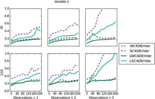
To compare these methods, we use as a metric the RMSE defined before. Figures 12, 13 and 14 show the RMSE for all methods for variables u, h and r, respectively.

In Fig. 12 we show comparisons for the methods on the velocity variable, u. The analysis RMSE of all methods increases the observation period increases. Over all observation densities (in time and space) we see that localisation gives improvement in RMSE over non-localised methods. This improvement is due to elimination of long distance spurious correlations (Whitaker and Hamill, 2002; Ott et al., 2004). At all observation periods, LWC4DEnVar out performs all other methods. As the observation period increases, both WC frameworks give a lower RMSE than their SC counterparts. This is expected because for longer windows the initial conditions become less important in the presence of model error.

Fig 12. This plot shows the RMSE (y-axis) of all data assimilation methods for velocity, u, and the x-axis is the observation period. In the top three plots, all grid points are observed and in the bottom three plots only 1 in 10 grid points are observed. The two plots on the left show one observation per window, the middle two show two observations per window and the two on the right show five observations per window.

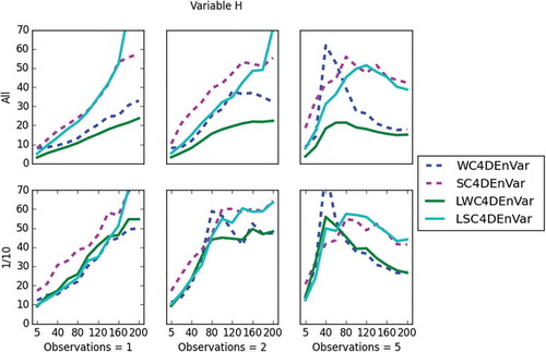
Figure 13 looks at the performance of the methods for the variable height, h. In the case where all grid points are observed (for u and h), localisation can be seen to improve the performance in all regimes with the WC framework. For the SC, the performance is improved with short observation periods and with all grid points observed, but as the observation period increases, this improvement deteriorates and in some cases LSC4DEnVar can be outperformed by SC4DEnVar. For sparse observations in space (observing 1:10 grid points), all methods perform similarly until the observation period length reaches a certain length. For observation periods greater than this length, the WC outperforms the strong constraint method. This is due to the slow nature of the height variable in the model. The accumulated model error develops slowly, giving the strong constraint a reasonable analysis in comparison. Once the accumulated model error has developed, the WC can help improve the analysis. Localisation with sparse observations (in space) shows little to no improvement. In all regimes, the LWC4DEnVar has a lower RMSE than all other methods except when observations are sparse (in space) and observation periods are small. Under this regime, all methods perform similarly.

Fig 13. This plot shows the RMSE (y-axis) of all data assimilation methods for height, h, and the x-axis is the observation period. In the top three plots, all grid points are observed and in the bottom three plots only 1 in 10 grid points are observed. The two plots on the left show one observation per window, the middle two show two observations per window and the two on the right show five observations per window.

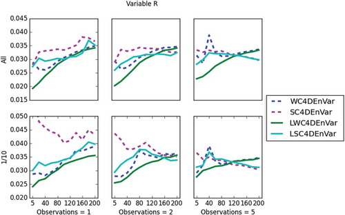
Finally, Fig. 14 presents the results for rain, r, which is our unobserved variable. Under all regimes (except five observations per window), localisation shows improvement in performance of the EnVar methods. The improvement is greater for smaller observation periods, then becomes less obvious as the observation period increases. For assimilation windows with five observations, localisation has no impact after an approximate observation period of 120 time steps. The localised versions outperform the non-localised ones in all regimes studied. The LWC4DEnVar outperforms the LSC4DEnVar in most regimes, except when the observation period is larger than 120 time steps. When the number of observations per window increases, LSC4DEnVar can outperform LWC4DEnVar. We have no clear argument on why this should be the case; this requires further study.

Fig 14. This plot shows the RMSE (y-axis) of all data assimilation methods for rain, r, and the x-axis is the observation period. In the top three plots, all grid points are observed and in the bottom three plots only 1 in 10 grid points are observed. The two plots on the left show one observation per window, the middle two show two observations per window and the two on the right show five observations per window.

5. Summary

In this paper we have explored the performance of a weak-constraint 4DEnsembleVar with and without localisation on the Lorenz 96 and a one-dimensional shallow-water model with simulated convection.

The most extensive and detailed experiments were performed using the imperfect L96 model with 24 variables. Simple experiments with observations every time step and at every grid point showed the importance of localisation for the ensemble and hybrid methods. We evaluated the time evolution of the analysis RMSE, as well as non-parametric statistics over 500 model steps. The variational, localised ensemble and localised hybrid methods were all able to achieve RMSE values lower than the observational error level.

We then proceeded to experiment with a more challenging set up: the land–sea configuration which includes 12 observed and 12 unobserved grid points. To analyse the results we divided the 24 grid points into three sets: eight ‘observed’ variables, eight ‘unobserved’ variables and eight ‘boundary’ variables. We took to observational frequencies: observations every time step and observations every two time steps. The results for both cases were similar. For this land–sea configuration it is clear how long-range spurious correlations can ruin the analysis for both boundary and unobserved variables leading to RMSE values larger than the climatological level. For the hybrid methods the introduction of localisation helps in the WC case, but it increases the RMSE for the SC case. This is similar to what we had observed in the case of the KdV experiments. It was shown how LSC4DEnVar has a very noisy time evolution for its analysis RMSE, while this evolution is considerably smoother for WSC4DEnVar. This behaviour is closer to that of the pure variational methods that use TLMs and AMs.

The last set of experiments with the L96 system aimed at testing the sensitivity to different parameters: ensemble size, localisation half-width, number of observational times in the assimilation window and number of outer loops. This was done over a larger time (1000 model steps). The experiments with LETKS showed that the permissible localisation half-width values reduce with the number of ensemble members, i.e. smaller ensembles must be localised more strictly. A very important finding for 4DVar was that, in the presence of model error which is ignored in the assimilation process—i.e. using SC4DVar, even though the model is imperfect—the use of outer loops can damage the assimilation. This is not the case with WC4DVar, which gives good and robust results in spite of using the approximate model-bias correction formulation to include model errors.

We finally experimented with the EnVar methods. Trying to mimic real situations, we focused our analysis on very small ensemble sizes. Localisation is indispensable to achieve good results, but we showed that it can severely damage the performance of LSC4DEnVar, especially in unobserved and boundary variables. This is not the case in LWC4DEnVar (except for the smallest ensemble size). For the observed variables, the results were in general better for LSC4DEnVar. The presence of outer loops damaged LSC4DEnVar, while the performance of LWC4DEnVar was largely unchanged and for some combinations of parameters it improved the performance of the method.

The SWE experiments have shown, in the presence of model error in systems that require localisation, how the WC framework helps to alleviate problems with the localisation of cross-time covariances which appear in the strong constraint framework. We have shown that the addition of a weak constraint generally improves the RMSE of 4DEnVar in cases where accumulated model error has time to develop, especially in cases where observations are sparse (in time and space).

6. Discussion

Numerical Weather Prediction (NWP) models are large and non-linear. Operational centres have started experimenting with hybrid methods, in particular the 4DEnVar, to try to improve forecast predictions (Fairbairn et al., 2014; Lorenc et al., 2015). On smaller models, 4DEnVar shows big improvements over traditional methods. In NWP problems are generated due to the non-linearity of the system and 4DEnVar, which uses temporal cross-covariances, excludes non-zero elements far from the diagonal in the covariance matrices when only spatial localisation is applied. The UK Met Office has tried to solve this problem using a hybrid background error covariance matrix over a climatologically generated background error covariance matrix as this can help incorporate errors of the day and add more flow-dependency to the background error covariance matrix. Meteo-France has tried to advect the localised background error covariances backwards with the flow to solve the localisation issues (Desroziers et al., 2016). This study used a simple model for Lagrangian advection, in which the authors had to balance the complexity of the advection model with the computational expense of the method.

In the present paper, we showed how adding a WC with localisation can be an effective way to track the evolution of the covariances, keeping a large part of the information which is lost in the SC framework.

Although these experiments show promising results for an LWC4DEnVar, there are several interesting areas for future work. The addition of incremental analysis updates (Bloom et al. 1996) could increase accuracy of the LWC4DEnVar by smoothing the trajectories over time. In terms of model error, our choice of the model error covariance matrix as can be improved and more accurately defined and we do not use any bias in the effective model error, which would be present in NWP. We have only considered model error increments at observation times. However, the true run has a stochastic input at every time step. Estimating these increments would lead to a more accurate estimation. For the moment, computational expenses (storage and operations) render this objective unworkable.

Acknowledgements

MG and PJvL acknowledge the support of the Natural Environment Research Council (NERC) via the National Centre for Earth Observations (NCEO) and also the DIAMET project (NE/I0051G6/1). JA and PJvL acknowledge the support of NERC (NE/I0125484/1) and NCEO. PJvL received funding from the European Research Council (ERC) under the European Union Horizon 2020 research and innovation programme.

Disclosure statement

No potential conflict of interest was reported by the authors.

Additional information

Funding

This work was supported by the Natural Environment Research Council; [NE/I0051G6/1]; NERC; [NE/I0125484/1]; NCEO; European Research Council (ERC).

References

- Bloom, S. C., L. L. Takacs, A. M. DaSilva, and D. Ledvina. 1996. Data assimilation using incremental analysis updates. Mon. Wea. Rev. 124, 1256–1271. DOI:10.1175/1520-0493(1996)124<1256:DAUIAU>2.0.CO;2.
- Desroziers, G., E. Arbogast, and L. Berre. 2016. Improving spatial localisation in 4DEnVar. Quart. Jour. of the Roy, Meteorol. Soc. DOI:10.1002/qj.2898.
- Fairbairn, D., S. Pring, A. C. Lorenc, and I. Roulstone. 2014. A comparison of 4DVar with ensemble data assimilation methods. Quart. Jour. of the Roy, Meteorol. Soc. 140, 281–294. DOI:10.1002/qj.2135.
- Hansen, J., and C. Penland. 2006. Efficient approximate techniques for integrating stochastic differential equations. Mon. Wea, Rev. 134, 3006–3014. DOI:10.1175/MWR3192.1.
- Lorenc, A. C., N. Bowler, A. Clayton, S. Pring, and D. Fairbairn. 2015. Comparison of Hybrid-4DEnVar and Hybrid-4DVar Data Assimilation Methods for Global NWP. Mon. Wea. Rev. 143, 212–229. DOI:10.1175/MWR-D-14-00195.1.
- Lorenz, E. 1996. Predictability—a Problem Partly Solved. Proc. Seminar on Predictability. Volume 1. European Centre for Medium-Range Weather Forecast. Shinfield Park, Reading, Berkshire, United Kingdom: Cambridge University Press.
- Lorenz, E. 2005. Designing chaotic models. J. of the Atmos. Sci. 62, 1574–1587. DOI:10.1175/JAS3430.1.
- Miyoshi, T. 2011. The Gaussian approach to adaptive covariance inflation and its implementation with the local ensemble transform Kalman filter. Mon. Wea. Rev. 139, 1519–1535. DOI:10.1175/2010MWR3570.1.
- Ott, E., B. Hunt, I. Szunyogh, A. Zimin, E. Kostelich, M. Corazza, E. Kalnay, D. Patiland, and J. Yorke. 2004. A local ensemble Kalman filter for atmospheric data assimilation. Tellus A. 56, 415–428. DOI:10.1111/j.1600-0870.2004.00076.x.
- Perianez, A., H. Reich, and R. Pottharst. 2014. Optimal Iocalization for Ensemble Kalman Filter systems. J. Meteorol. Soc. Jpn. 92, 585–597. DOI:10.2151/jmsj.2014-605.
- Tremolet, Y. 2004. Diagnostics of linear and incremental approximations in 4D-Var. Q. J. R. Meteorol. Soc. 130, 2233–2251. DOI:10.1256/qj.03.33.
- Tremolet, Y. 2006. Accounting for an imperfect model in 4D-Var. Q. J. R. Meteorol. Soc. 132, 24832504.
- Tremolet, Y. 2007. Incremental 4D-Var convergence study. Tellua A. 59, 706–718. DOI:10.1111/j.1600-0870.2007.00271.x.
- Whitaker, J. S., and T. M. Hamill. 2002. Ensemble data assimilation without perturbed observations. Mon. Wea. Rev. 130, 1913–1924. DOI:10.1175/1520-0493(2002)130<1913:EDAWPO>2.0.CO;2.
- Wursch, M., and G. Craig. 2014. A simple dynamical model of cumulus convection for data assimilation research. Meteorologische Zeitschrift. 23, 483–490.
- Yang, S.-C., D. Baker, H. Li, K. Cordes, M. Huff, G. Nagpal, E. Okereke, J. Villafane, E. Kalnay, and G. Duane. 2006. Data assimilation as synchronization of truth and model: Experiments with the three-variable Lorenz system. J. of the Atmos. Sci. 63, 2340–2354. DOI:10.1175/JAS3739.1.