
Abstract
Ensemble methods such as the Ensemble Kalman Filter (EnKF) are widely used for data assimilation in large-scale geophysical applications, as for example in numerical weather prediction. There is a growing interest for physical models with higher and higher resolution, which brings new challenges for data assimilation techniques because of the presence of non-linear and non-Gaussian features that are not adequately treated by the EnKF. We propose two new localized algorithms based on the Ensemble Kalman Particle Filter, a hybrid method combining the EnKF and the Particle Filter (PF) in a way that maintains scalability and sample diversity. Localization is a key element of the success of EnKF in practice, but it is much more challenging to apply to PFs. The algorithms that we introduce in the present paper provide a compromise between the EnKF and the PF while avoiding some of the problems of localization for pure PFs. Numerical experiments with a simplified model of cumulus convection based on a modified shallow water equation show that the proposed algorithms perform better than the local EnKF. In particular, the PF nature of the method allows to capture non-Gaussian characteristics of the estimated fields such as the location of wet and dry areas.
1. Introduction
In many large-scale environmental applications, estimating the evolution of a geophysical system, such as the atmosphere, is of utmost interest. Data assimilation solves this problem iteratively by alternating between a forecasting step and an updating step. In the former, information about the dynamic of the system is incorporated, while in the latter, also called analysis, partial and noisy observations are used to correct the current estimate. The optimal combination of the information from these two steps requires an estimate of their associated uncertainty. In statistics, one represents the uncertainty about the state of a system after the forecasting step with a prior distribution, and the uncertainty due to the observations errors with a likelihood. The analysis consists then in deriving the posterior distribution of the current state of the system, combining the prior distribution and the new observations, which can be done with Bayes’ rule.
In geophysical applications, such as numerical weather prediction (NWP), the dimension of the system is extremely large and the forecasting step computationally heavy, therefore the focus is on developing efficient methods with reasonable approximations. Even in the simplest case of a linear system with linear Gaussian observations, the optimal method, namely the Kalman filter (Kalman, Citation1960; Kalman and Bucy, Citation1961), is difficult to use because of the size of the matrices involved.
Ensemble, or Monte-Carlo, methods, are elegant techniques to deal with non-linear dynamical systems. They use finite samples, or ensembles of particles, to represent the uncertainty about the state of the system associated with the prior and posterior distributions. The forecasting step consists then simply in integrating each particle according to the law of the system. Ensemble methods were introduced in the geosciences by the Ensemble Kalman Filter (EnKF) of Evensen (Citation1994, Citation2009) as a Monte-Carlo approximation of the Kalman filter and have shown great success in practice. However, the analysis step of all EnKF methods implicitly relies on the assumption that the prior uncertainty about the state of the system is Gaussian, which is an acceptable approximation in some cases, but is unlikely to hold with highly non-linear dynamics.
Particle Filters (PFs) (Gordon et al., Citation1993; Pitt and Shephard, Citation1999; Doucet et al., Citation2001) are a more general class of ensemble methods which differ from the EnKF in the way the analysis step is implemented. They can handle fully non-linear and non-Gaussian systems and are therefore very attractive. Unfortunately, it has been shown that the number of particles needed to avoid sample degeneracy and collapse of the filter increases exponentially with the size of the problem, in a sense made precise in Snyder et al. (Citation2008). Adapting PFs for large-scale environmental applications is an active field of research andthere are many propositions of algorithms (see van Leeuwen (Citation2009) for a review, and van Leeuwen (Citation2010); Papadakis et al. (Citation2010); Ades and van Leeuwen (Citation2013); Nakano (Citation2014) for more recent developments). Here we focus on the Ensemble Kalman Particle Filter (EnKPF), introduced in Frei and Künsch (Citation2013), which consists in a combination of the PF with the EnKF. Compared to other similar algorithms, the EnKPF has the distinct advantage of being dependent on a single tuning parameter which defines a continuous interpolation between the EnKF and the PF. Moreover, no approximation of the prior distribution or the transition probability is required.
Recently, there has been a tendency towards using physical models with higher and higher resolution. For example in NWP, regional models are starting to be run with a grid length of the order of 1 km, which allows to resolve explicitly highly non-linear phenomena such as cumulus convection. In general, with non-linear dynamical systems, the uncertainty after the forecasting step can become highly non-Gaussian. Therefore there is a growing need for data assimilation methods which can handle non-linear and non-Gaussian systems while being computationally efficient to be applied to large-scale problems (Bauer et al., Citation2015). The EnKF implicitly assumes Gaussian uncertainty while the PF requires an exponentially large number of particles. The EnKPF is a compromise between both, but it still requires too many particles for practical applications. The main goal of this article is to contribute towards a full solution to the non-linear and non-Gaussian large-scale data assimilation problem.
The methods proposed in this article expand on the EnKPF by introducing localization. The idea of localizing the analysis was first proposed by Houtekamer and Mitchell (Citation1998) as a device to reduce dimensions and thus to allow for smaller ensemble sizes. While localization has been widely used within the EnKF family of algorithms, e.g. the Local Ensemble Transform Kalman Filter (LETKF) of Hunt et al. (Citation2007), applications to the PF are much rarer. The reason for this is that PF methods introduce a discrete component in the analysis by resampling particles, which breaks the necessary smoothness of the fields to be estimated.
In the literature, the main approaches to this problem have been either to avoid resampling altogether, or to correct the introduced discontinuities. The moment-matching filter of Lei and Bickel (Citation2011) avoids resampling and can be localized straightforwardly as it depends on the first two moments of the distribution only. Attempts to replace resampling by deterministic transport maps from prior to posterior distributions are a promising way to reformulate PFs such that they can be easily localized (Reich, Citation2013). An early example of algorithm which keeps resampling while localizing the analysis is the local-local ENSF (LLENSF) of Bengtsson et al. (Citation2003), with which our new algorithm share many similarities. In the recent local PF of Poterjoy (Citation2016) resampling is applied locally by progressively merging resampled particles with prior particles, followed by a higher order correction using a deterministic probability mapping.
In this article, we propose two new localized algorithms based on the EnKPF: the naive-local EnKPF (NAIVE-LEnKPF) and the block-local EnKPF (BLOCK-LEnKPF). In the NAIVE-LEnKPF, assimilation is done independently at each location, ignoring potential problems associated with discontinuities; in the BLOCK-LEnKPF, data are assimilated by blocks, whose influence is limited to a neighbourhood, and discontinuities are smoothed out in a transition area by conditional resampling. The first method is easier to implement as it mirrors the behaviour of the LETKF, but the second one deals better with the specific problems associated with localized PFs. The localization of the EnKPF or any PF method is highly non-trivial, but it can potentially bring remarkable improvement in terms of their applicability to large-scale applications (Snyder et al., Citation2015).
The original EnKPF has been shown in Frei and Künsch (Citation2013) to perform well on the Lorenz 96 model (Lorenz and Emanuel, Citation1998) and other rather simple setups. The extensions that we propose in the present paper should allow the algorithm to work on more complex and larger models. Here, we test the feasibility of our methods with some numerical experiments on an artificial model of cumulus convection based on a modified shallow water equation (SWEQ) (Würsch and Craig, Citation2014) and show that we obtain similar or better results than the EnKF.
In Section 2 we briefly review ensemble data assimilation and the EnKF, the PF and the EnKPF. Then we discuss localization and explain the two new localized EnKPFs algorithms in Section 3. The numerical experiments and the results are discussed in Section 4. Conclusions are presented in Section 5.
2. Ensemble data assimilation
Consider the problem of estimating the state of a system at time t, , given a sequence of partial and noisy observations
. The underlying process
is unobserved and represents the evolution of the system, described typically by partial differential equations. The observations are assumed to be conditionally independent given the states and are characterized by the likelihood
. This problem fits in the framework of general state space models and is generally known as filtering in the statistics and engineering community, and as data assimilation in the geosciences.
Mathematically, the goal is to compute the conditional distributions of given
, called the filtering or analysis distribution
. There exists a recursive algorithm which alternates between computing the analysis distributions and the conditional distributions of
given
, called the predictive or background distribution
. In the forecast step, the background distribution at time t is derived from the analysis distribution at time
, using the dynamical laws of the system. In the analysis or update step, the analysis distribution at time t is derived from the background distribution at the same time t, using Bayes’ theorem:
. However, there is no analytically tractable solution to this recursion except in the case of a discrete state space or a linear and Gaussian system. In the latter case, the solution is known as the Kalman filter.
One of the problems that arise when trying to apply this theoretical framework to large-scale systems such as in NWP is that the forecast step is not given by an explicit equation but comes from the numerical integration of the state vector according to the dynamical laws of the system. Ensemble or Monte Carlo methods address this problem by representing the distributions and
by finite samples or ensembles of particles:
and
for
, where k is the size of the ensemble. The forecast step produces the background ensemble members
by propagating the analysis ensemble members
according to the dynamics of the system. The analysis step, that is the transformation of the background ensemble
into the analysis ensemble, is however more challenging for ensemble methods. There are various solutions to this problem, depending on the assumptions about the distribution
and the observation process and the heuristic approximations that are used.
Henceforth we drop the time index t and consider the analysis step only. We also assume that the observations are Gaussian and linear with mean Hx and covariance R, where H is the observation operator applied on a state vector x and R is a valid covariance matrix. We now review the EnKF and the PF in this context and describe the EnKPF, before discussing in more detail the problem of localization and introducing new algorithms.
2.1. The Ensemble Kalman Filter
If one assumes that the background distribution is Gaussian and that the observations are linear and Gaussian, then the analysis distribution
is again Gaussian with a new mean and covariance given by simple formulae. All EnKF methods are based on this result and apply it by ignoring non-Gaussian features of
. They use the background ensemble to estimate the mean and covariance of
and draw the analysis sample to match the mean and covariance of
under Gaussian assumptions. Square-root filters such as the LETKF transform the background ensemble so that the first and second moments match exactly those of the estimated analysis distribution, whereas the stochastic EnKF applies a Kalman filter update with some stochastically perturbed observations to each ensemble member. More precisely, in the stochastic EnKF an ensemble member from the analysis distribution is produced as follows:
(1)
where is an estimate of the background covariance matrix and
is a vector of observation perturbations. K(P) denotes the Kalman gain computed using the covariance matrix P and is equal to
. Conditional on the background ensemble
,
is thus normal with mean
and covariance
. A key idea for the EnKPF is that, conditional on the background ensemble, the analysis ensemble is a balanced sample of size k from the Gaussian mixture
(2)
where balanced sample means that each component of the mixture is selected exactly once.
2.2. The Particle Filter
The PF does not make any assumption about , but applies Bayes’ formula to the empirical distribution provided by the background ensemble. In its simplest version it represents the background and analysis distributions by weighted samples of particles, whose weights are updated at each time step by a factor proportional to the likelihood of the observations. That is, if
is represented by the weighted sample
, then
is represented by the weighted sample
, where
In the forecast step, weights remain unchanged. However, when iterated this leads to sample degeneracy, that is the weights are effectively concentrated on fewer and fewer ensemble members. To avoid this, a resampling step is introduced, where the particles are resampled with probability proportional to their weight. This means that the analysis sample contains times where
and
. In this way particles which fit the data well are replicated and the others eliminated, thus allowing to explore adaptively the filtering distribution by putting more mass in regions of high probability.
There are balanced sampling schemes, where , which reduce the error due to resampling as much as possible (discussion of balanced sampling can be found inCarpenter et al. (Citation1999); Crisan (Citation2001) or Künsch (Citation2005)). But resampling also has problems with sample depletion if the likelihood values
are very unbalanced or the dynamical system is deterministic. In that case one has to add some kind of perturbations to the analysis particles, but it is not clear how to choose the covariance of this noise.
Using a vector of resampled indices I, such that and
for all j, we can write the PF algorithm succinctly as follows:
| (1) | Compute the weights | ||||
| (2) | Choose the vector of resampled indices I, such that | ||||
| (3) | For | ||||
2.3. The Ensemble Kalman Particle Filter
The EnKPF (Frei and Künsch, Citation2013) is a hybrid algorithm that combines the EnKF and the PF with a single parameter controlling the balance between both. Its core idea is to split the analysis in two stages, following the progressive correction principle of Musso et al. (Citation2001). In a nutshell, the algorithm consists in ‘pulling’ the ensemble members towards the observations with a partial EnKF analysis using the dampened likelihood
, and then applying a partial PF with the remaining part of the likelihood,
. In this way the algorithm can capture some non-Gaussian features of the distribution (by resampling), while maintaining sample diversity. For any fixed
, it does not converge to the true posterior distribution as the number of particles tends to infinity, unless the background distribution is Gaussian. The justification of the EnKPF is rather that, for non-Gaussian background distributions, it reduces the variance of the PF at the expense of a small bias.
We now review the derivation of the algorithm briefly but refer to Frei and Künsch (Citation2013) for more detail. Assuming linear and Gaussian observations, dampening the likelihood with the exponent is equivalent to inflating the error covariance R by the factor
, and it is easily seen that this is also equivalent to using the Kalman gain with the original error covariance R and a dampened background covariance
. From the Gaussian mixture representation of the EnKF analysis described in Equation (Equation2
(2) ), we can see that the first step of the algorithm produces the partial analysis distribution
(3)
where(4)
(5)
For the second step, we have to apply Bayes’ formula using as the prior and
as the likelihood. This has a closed form solution (Alspach and Sorenson, Citation1972), namely a Gaussian mixture with new centroids
, covariance
, and unequal weights
:
(6)
where(7)
(8)
(9)
and denotes the density of a Gaussian with mean
and covariance matrix
evaluated at y. One can rewrite the equation for the
components directly from the background ensemble as:
(10)
The final analysis sample is obtained as a sample from the Gaussian mixture (Equation6(6) ), which can be done at a computational cost comparable to the EnKF. A short description of the algorithm is given as follows:
| (1) | Compute all the | ||||||||||||||||
| (2) | Compute all the weights | ||||||||||||||||
| (3) | Choose the vector of resampled indices I, such that | ||||||||||||||||
| (4) | For
| ||||||||||||||||
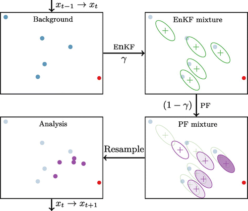
Figure 1. Schematic illustration of the EnKPF. Upper left: Background ensemble (blue dots) and observation (red dot). Upper right: Intermediate analysis distribution (Equation3
(3) ). Each ellipse covers 50% of one component in the mixture. Lower right: Final analysis distribution Equation (Equation6
(6) ). Ellipses again represent 50% of each component, and the colour intensity represents the weights
. Lower left: Analysis sample obtained by drawing from Equation (Equation6
(6) ). The mixture component closest to the observation has been resampled three times, while the two components farthest away have been discarded.
In the extreme case of , the EnKPF is equivalent to a pure PF, whereas for
it is equivalent to the stochastic EnKF.
is therefore a tuning parameter which determines the proportion of EnKF and PF update to use. In practice it is chosen adaptively such that the ensemble is as close as possible to the PF solution while conserving enough diversity. Diversity of the mixture weights
can be quantified by the Effective Sample Size (ESS) (Liu, Citation1996).
The EnKPF has been shown to work well with the Lorenz 96 models and with other simple examples (Frei and Künsch, Citation2013). However, because it has a PF component, it cannot be directly applied to large-scale systems without suffering from sample degeneracy. In the following section we discuss the technique of localization and introduce two new localized algorithms based on the EnKPF.
3. Local algorithms
One of the key element for the success of the EnKF in practice is localization, either by background covariance tapering as in Hamill et al. (Citation2001), or by doing the analysis independently at each grid point, using only nearby observations, as in Ott et al. (Citation2004). Localization suppresses spurious correlations at long distances and generally increases the statistical accuracy of the estimates by reducing the size of the problem to solve. Its drawback, however, is that it can easily introduce non-physical features in the global analysis fields. For the Local Ensemble Kalman Filter (LEnKF) such problems are reduced by ensuring with some means that the analysis varies smoothly in space. It should be noted that physical properties of the global fields cannot be guaranteed in a strong sense without incorporating some explicit constraints.
Without Gaussian assumptions localization becomes even more crucial but also more difficult, as the analysis does not anymore depend on the background mean and covariance only. The collapse of the PF with small ensemble sizes could be avoided by using a very strong localization. However, a pure local PF would probably not be practical as it would introduce arbitrarily large discontinuities in the analysis since different particles can be resampled at neighbouring grid points and need to be glued together.
Localizing the EnKPF is easier than for a pure PF but it still requires some care due to the resampling step. We propose two different localized algorithms based on the EnKPF: the first one is based on the same principle as the LEnKF of Ott et al. (Citation2004), while the second one is closer to the idea of covariance tapering of Hamill et al. (Citation2001) and serial assimilation of Houtekamer and Mitchell (Citation2001), but adapted to the PF context.
3.1. The naive-local ENKPF
In the NAIVE-LEnKPF, we apply the exact same approach as in the LEnKF of Ott et al. (Citation2004) and do an independent analysis at each grid point. We call the resulting algorithm naive because it ignores dependencies between grid points. More precisely, the analysis at a given site is produced by sampling from a local analysis distribution which has the same form as Equation (Equation6(6) ), but which is computed only using observations close to this site. As in the LEnKF, some level of smoothness is ensured by using the same perturbed observations at every grid point and by choosing a local window large enough such that the observations assimilated do not change too abruptly between neighbouring grid points.
In order to mitigate the problem of discontinuities further, we introduce some basic dependency by using a balanced sampling scheme with the same random component for every grid point and by reordering the resampling indices such that the occurrence of such breaks is minimized. This does not remove all discontinuities, but essentially limits them to regions where the resampling weights of the particles change quickly.
In conclusion, the NAIVE-LEnKPF has the advantage to be straightforward to implement, following closely the model of the LEnKF, but it is not completely satisfactory as it introduces potential discontinuities in the global analysis fields. We now consider a second algorithm which is a bit more complicated but avoids this problem.
3.2. The block-local EnKPF
In the NAIVE-LEnKPF, localization consists in doing a separate analysis at each grid point, using the observations at nearby locations. We now consider another approach to localization, in which the influence of each observation is limited to state values at nearby locations. This seemingly innocuous change of perspective leads to the development of a new algorithm, the BLOCK-LEnKPF. Assuming that R is diagonal or block-diagonal, the observations y can be partitioned into disjoint blocks and then assimilated sequentially, as for example in the EnKF of Houtekamer and Mitchell (Citation2001). The way that localization is implemented for the BLOCK-LEnKPF is similar in spirit to the global-to-local adjustment of the LLENSF of Bengtsson et al. (Citation2003), but the derivation and the resulting algorithms are not identical.
In the case of the EnKF, the influence of one block of observations can be limited to a local area by using a tapered background covariance matrix (Hamill et al., Citation2001). However, only in the Gaussian case, setting correlations to zero implies independence, but for general this is not true. The PF and EnKPF maintain higher order dependencies by resampling particles globally, but with a local algorithm some dependencies will necessarily be broken. The BLOCK-LEnKPF maintains these dependencies when it is possible, but falls back on a conditional EnKF and implicitly relies on Gaussian assumptions to bridge discontinuities when they are unavoidable. We now describe in more detail how to derive the algorithm for one block of observations and then discuss the general method and parallel assimilation.
3.2.1. Assimilation of one block of observations
Let us say we partitioned the observations into B blocks and want to assimilate . If we assume that the observation operator is local, then only a few elements of the state vector influence the block
directly (i.e. have non-zero entry in H for a linear operator). We denote their indices by u with corresponding state vector
. Hereafter we use subscripts to denote subvectors or submatrices.
Let us assume also that we use a valid tapering matrix C, for example the one induced by the correlation function given in Gaspari and Cohn (Citation1999). We denote by the subvector of elements that do not influence
, but are correlated with some elements of
(i.e. correspond to non-zero entries in the tapering matrix C). Additionally, we define as
the subvector of all remaining elements.
The principle of the algorithm is to first update with the EnKPF while keeping
unchanged. In a second step,
is updated conditionally on
and
, such that potential discontinuities are smoothed out. If
and
are not only uncorrelated, but also independent, the background distribution can be factored as:
(11)
By construction, only influences
so that one can write
. Applying Bayes’ rule, the analysis distribution is
A natural way to sample from this distribution goes as follows: (i) sample from the analysis distribution
, (ii) keep
unchanged and (iii) sample
from
, conditionally on
and
. Steps (i) and (iii) are clear, but (ii) requires more discussion.
One could assume normality and sample as a random draw from a normal distribution with the conditional mean and covariance computed from the background sample moments. However this would add unnecessary randomness and it is more judicious to sample
as a correction to the background ensemble member
, as is done in the EnKF. Using this sampling scheme, we can show that the analysis of
conditioned on
and
is given by the following simple expression:
(12)
where the matrix inverse is well defined if a tapered estimate of is used, and should be understood as a generalized inverse otherwise.
At first sight it is puzzling that does not appear in the formula, but the correlation between
and
is present in the background sample
and thus does not need to be explicitly taken into account in the analysis. Note that
depends on
.
In cases where , the entire particle
is therefore obtained as a correction of the entire particle
, according to the original EnKPF algorithm. In cases where
,
will depend on two background particles
and
and the analysis relies on additional Gaussian assumptions of the background sample. Formula (Equation12
(12) ) then makes sure that the correlation between
and
is nevertheless correct. In order to stay as close as possible to the EnKPF, we permute the resampling indices I(i) such that the number of cases with
is maximal. More details about the derivation of the algorithm are provided in Appendix .
Putting everything together, the assimilation of one block of observations in the BLOCK-LEnKPF algorithm can be summarized as follows:
| (1) | Compute all the | ||||||||||||||||||||||||||||
| (2) | Compute all the weights | ||||||||||||||||||||||||||||
| (3) | Choose the vector of resampled indices I, such that | ||||||||||||||||||||||||||||
| (4) | Permute I such that | ||||||||||||||||||||||||||||
| (5) | For
| ||||||||||||||||||||||||||||
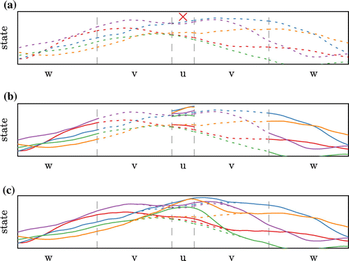
Figure 2. Illustration of the assimilation of one observation (red cross in panel (a)) with the BLOCK-LEnKPF. Each particle is shown in a different colour, the dotted lines being the background and the solid lines the analysis. In panel (b) is updated while
is unchanged. In panel (c) we see how the update in
makes a transition between
and
. For the orange and green particles, which are not resampled in
, the analysis has to bridge between two different particles by relying on Gaussian assumptions as described in Appendix .
3.2.2. Parallel assimilation of observations
In the previous paragraph we described how one block of observations is assimilated in the BLOCK-LEnKPF. Now let us consider the case of two blocks of observations to be assimilated, say and
. Defining the corresponding state vector indices as above and using an additional subscript for the block, we can see that if
, then in principle parallel instead of serial assimilation of
and
is possible. In the case where
and
are contiguous, one might worry about discontinuities at the boundary between
and
. However, the tapering matrix C ensures that the correlations between sites near this boundary and sites in
and
is small and thus the parallel assimilation of
and
through Equation (Equation12
(12) ) makes only small changes near this boundary. The procedure could however introduce some discontinuities in higher order dependence between
and
. To avoid this, one could require an additional buffer area between
and
, but it would slow down the algorithm and most likely not bring much improvement.
We can therefore assimilate all blocks of observations where the corresponding sets u are well separated in parallel. However, blocks where the corresponding sets u are close have to be assimilated serially. In theory, each assimilation of one block increases the correlation length because the analysis covariance becomes the new background covariance, but we neglect this increase and continue using the same taper matrix C until all observations have been assimilated. This additional approximation is necessary to keep the filter local and it is also used in the serial LEnKF of Houtekamer and Mitchell (Citation2001). The resulting algorithm can be described more precisely as follows:
| (1) | Partition the observations in B blocks | ||||
| (2) | Choose a block i which has not been assimilated so far or exit if none is left. | ||||
| (3) | Assimilate in parallel | ||||
| (4) | Go to step (2). | ||||
To recapitulate, the BLOCK-LEnKPF consists in assimilating data by blocks and in limiting their influence to a local area. The analysis at sites that do not directly influence the observations in the current block but are correlated with is done by drawing from the conditional background distribution. For cases where resampling does not occur, doing so is equivalent to applying EnKPF in the local window, whereas for cases where it does occur, the algorithm avoids to introduce harmful discontinuities and produces a smoothed analysis. The BLOCK-LEnKPF satisfies all our desiderata for a successful localized algorithm based on the EnKPF. Its disadvantage, however, is that it requires more overhead for the partitioning of observations and its implementation in an operational setting is more complicated.
Now that we introduced two new localized algorithms based on the EnKPF, we will proceed to numerical experiments in order to better understand their properties and test their validity by comparing their performance to the LEnKF.
4. Numerical experiments
The algorithms introduced in the present paper can be applied to any task of data assimilation for large-scale systems. However we expect that relaxation of Gaussian assumptions will be most beneficial when the dynamical system is strongly non-linear. Such an application is data assimilation for NWP at convective scale. Würsch and Craig (Citation2014) introduced a simple model of cloud convection which allows one to quickly test and develop new algorithms for data assimilation at convective scale (as e.g. in Haslehner et al. (Citation2016)). We first briefly introduce the model and the mechanism to generate artificial observations. Then we present results of two cycled data assimilation experiments.
4.1. The modified shallow water equation model
The model is based on a modified SWEQ on a one-dimensional domain to generate patterns that are similar to the creation of convective precipitations in the hot months of summer. The convective cells are triggered by plumes of ascending hot air generated at random times and locations. The SWEQ is modified in such a way that if h, the height of the fluid, in the present case humid air, reaches a given threshold () the convection is reinforced and leads to the creation of a cloud. The convection mechanism is maintained until the fluid reaches a new threshold (
), above which the cloud starts to produce rain at a given rate and then slowly disappears. The state of the system can thus be described by three variables: the fluid height h, the rain content r and the horizontal wind speed u. We do not use any units as the scales are arbitrary.
The parameters (fluid height thresholds, precipitation rate, etc.) are the same as for the model run described in Würsch (Citation2014, Chap. 5) except for the cloud formation threshold set to as in Würsch and Craig (Citation2014). They have been tuned so that the system exhibits characteristics similar to real convection (fraction of clouds, life-time of precipitation, etc). The random perturbations are introduced at a rate of
. We use a domain size of 150 km with periodic boundary conditions and a resolution of 500 m.
From this system we generate artificial observations that imitate radar measurements. In order to make the experiment realistic, we use a non-linear and non-Gaussian mechanism for generating the observations, but consider them as linear and Gaussian during the assimilation. The rain field is observed at every grid point, but set to zero if below a threshold (), and with some skewed error whose scatter increases with the average amount of rain otherwise. Our observation mechanism is different from the one of Würsch and Craig (Citation2014), where simple truncated Gaussian errors were used, and is intended to be more realistic and challenging than the latter. In more detail, the rain observations
are generated as follows:
where , independently at every grid point. Such a skewed error distribution for rain observations is a common choice (see e.g. Sigrist et al. (Citation2012); Stidd (Citation1973)). It consists in applying a Box-Cox transform (with parameter
), adding some white noise and then transforming back to the original scale. Besides rain, wind speed is also observed with some additive Gaussian noise (with variance
), but only at grid points where the observed rain is positive (
). For the present experiment
and
.
Such artificial observations make data assimilation realistic and challenging due to the non-linearity and sparsity of the observation operator and the non-Gaussian errors. One could consider transforming the observations to obtain a more normal distribution, but we want to test if our algorithms can handle such difficult situations.
Figure 3. Typical example of the modified SWEQ model with artificial radar observations (red dots) and critical values (,
and
) as dashed lines.
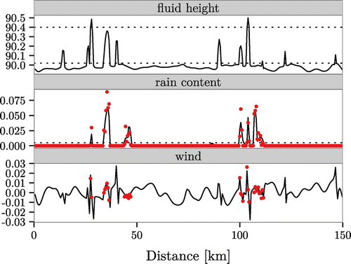
A typical example of a field produced with the model and some artificial observations is displayed in Fig. . The bumps in fluid height represent clouds which start to appear if the first threshold is reached (lower dashed line) and are associated with precipitation if they reach the second threshold (upper dashed line), after which they start to decay. Rain can remain for some time after a cloud has reached its peak. The sharp perturbations in the wind field are the random triggering plumes.
4.2. Assimilation setup
An initial ensemble of 50 members is generated by letting the model evolve without assimilating any observations and taking each member at 200 days interval from each other such that they are not correlated. We consider only perfect model experiments and do not take into account model error; in particular we do not use any form of covariance inflation. All the observations are assumed to be Gaussian, with a diagonal covariance matrix R with non-zero elements or
, depending on which type of observations it corresponds to. For wind observations the error is the same as for the true generating process, that is we set
. Rain and no-rain observations are both assimilated and assumed to have the same error. The true rain distribution is non-Gaussian, so
is not straightforward to choose, especially because it depends on the rain level. We set
during the assimilation, which is equivalent to the error observed for a rain level of 0.06125 (relatively big, but in the range of observed values). In general more could be done to treat rain observations properly, but it is beyond the scope of the present study.
We use one localization parameter l set to 5 km. Every method uses a taper of the covariance matrix as defined in Gaspari and Cohn (Citation1999) with half correlation length l. For LEnKF and NAIVE-LEnKPF, the size of the local window is set to l in each direction, for a total of approximately 10 km or 21 grid points. Similarly, the observation blocks for the BLOCK-LEnKPF are defined from segments of 10 km in the domain (one block contains all the rain observations falling in a specific 10 km segment and the associated wind observations, if any).
The EnKPF has one free parameter, , which controls the balance between EnKF and PF. We choose it adaptively such that the ESS at the resampling step is between 50 and 80% of the ensemble size. A different
can be selected for each site in the case of the NAIVE-LEnKPF, or for each block of observations for the BLOCK-LEnKPF, which allows the method to be closer to the PF in regions where non-Gaussian features are present and to fall back closer to the EnKF when it is necessary. In general the criterion for adaptive
could be refined and tuned more closely, but it is beyond the scope of the present paper.
The two new local algorithms are compared against the LEnKF of Ott et al. (Citation2004) and not the LETKF of Hunt et al. (Citation2007), because both the EnKPF and the LEnKF are based on the stochastic EnKF and thus are more comparable. Furthermore our results cannot be directly compared to the ones in Haslehner et al. (Citation2016) as our experimental set-up is substantially different from theirs.
4.3. Results
In order to highlight some key properties of the new proposed algorithms, we start with an example where high-frequency observations are assimilated and study the resulting analysis ensembles visually. In a second step, repeating this experiment many times, we can evaluate the performance of the algorithms and their differences. In a third step we discuss longer assimilation periods with lower frequency observations. We show the results as figures only as we believe that they are only indicative of some possible advantages but should not be taken too literally as the system under study is very artificial and the results can vary with different choice of parameters. The quality of assimilation is assessed with the continuous ranked probability score (CRPS) (Gneiting and Raftery, Citation2007) commonly defined as:
where is the predictive cumulative probability function, in our case given by the empirical distribution of the ensemble. Because we have a perfect model scenario we can directly evaluate the CRPS of the one-step ahead forecast ensemble compared to the underlying true state of the system. The CRPS is a strictly proper scoring rule, which implies that using such a score allows one to control calibration and sharpness at the same time, contrary to the more commonly used rmse (see Gneiting and Katzfuss (Citation2014) for a general discussion of probabilistic forecasting).
4.3.1. High-frequency observations
In this first scenario we are interested in seeing if it is possible to use high-frequency radar data, especially for short-term prediction. To do so we run a cycled experiment where data are assimilated every 5 min for a total of 1 h. Starting from an initial ensemble which has no information about the current meteorological situation, the goal of the filter is to quickly capture areas of rain from the observations.
The analysis ensembles of the different algorithms for the rain field show that the local EnKPFs are better able to identify dry areas. In Fig. we can see the analysis ensembles after 1 h of assimilation in the same typical situation as in Fig. . All methods recover the zones of heavy precipitation relatively well, with some minor differences in terms of maximum intensity. One should not conclude too much from an isolated case, but there is one interesting trait which is not peculiar to this example and illustrates how the local EnKPF algorithms are able to model non-Gaussian features: the LEnKF maintains some medium level of rain at almost all sites, while both NAIVE-LEnKPF and BLOCK-LEnKPF are better at using the no-rain observations to suppress spurious precipitation.
Going beyond this particular example, we now consider a simulation study where we repeated the above experiment 1000 times and computed the average CRPS of each algorithm for every assimilation cycle. To make the results more understandable and to remove some natural variability, we always compute the performance relative to a free forecast run. The latter is based on the same initial ensemble used by all algorithms, but does not assimilate any observation, and is thus equivalent to a climatological forecast.
Both new algorithms achieve good performances compared to the LEnKF for the first hour of assimilation, as can be seen in Fig. . The gains are in terms of rain content, probably because it is the field with the most non-Gaussian features. The BLOCK-LEnKPF seems to have a slight advantage over the NAIVE-LEnKPF for the fluid height and the other way round for the rain field, but otherwise their performance is very similar.
Figure 4. Typical example of analysis ensembles for the rain field after 1 h of high-frequency observations assimilation. Each of the red line is one ensemble member. On top is the LEnKF, followed by the NAIVE-LEnKPF and the BLOCK-LEnKPF.
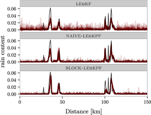
Figure 5. Evolution of the CRPS in the first hour with high-frequency observations. The value is given as a percentage relative to a free forecast run. Notice the truncated y-axis.
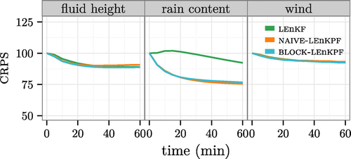
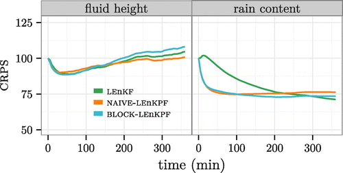
Interestingly, if one looks at the evolution of the CRPS for an assimilation period of 6 h instead of only 1 h in Fig. , some issues start to become apparent. After an initial drop, the CRPS for the fluid height field increases again and gets worse than the free forecast reference, which means that observations actually hamper the algorithms. The effect is greatest for the fluid height but also slightly visible for the rain for the NAIVE-LEnKPF. Physically, the problem comes from the fact that there is a delay between the formation of a cloud and the appearance of rain. Having assimilated many no-rain observations the algorithm can become overconfident that an area is dry and cannot adapt when new rain starts to appear. The LEnKF is a bit less susceptible to this problem, for the simple reason that it is less good at identifying dry areas and thus maintains more spread in the ensemble while the local EnKPFs are too sure that no rain is present. Such an effect can be understood as a form of sample degeneracy coming from the fact that a large number of observations are assimilated, which will be confirmed in the next experimental set-up.
Figure 6. Evolution of the CRPS (relative to a free forecast run) for the fluid height and rain fields in the first 6 h with high-frequency observations. It becomes obvious that after the first initial improvement, all algorithms deteriorate in terms of their ability to capture the underlying fluid height. Notice the truncated y-axis.
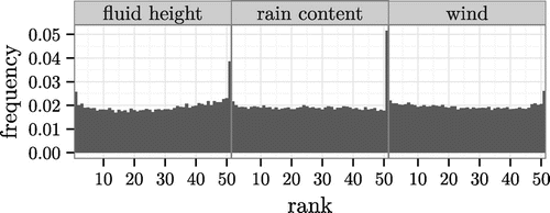
To assess the calibration of the algorithms we also look at the rank histograms of all fields in the first hour of assimilation for the BLOCK-LEnKPF in Fig. . The one-step ahead forecast is more or less calibrated, except for a non-negligible fraction of cases where the truth lies outside the range of the ensemble. These problems can be attributed to the inherent difficulty coming from the fundamentally random nature of the system. Indeed, attempts at improving the calibration with covariance inflation and tuning of the R matrix have not been successful. The histograms for the fluid level and the rain content reveal that some newly appeared clouds are missed, while some spurious clouds are sometimes created. The histogram for the absolute wind speed is generally uniform except for a slight underestimation, which comes from the random perturbations of the wind field. Conclusions are similar for other algorithms and no clear differences can be identified. Therefore, the improvements in CRPS can be interpreted mainly as better sharpness while keeping calibration the same.
Figure 7. Rank histograms computed at one-step ahead forecast for the BLOCK-LEnKPF in the high-frequency observations experiment. Only every 10 grid points and every 30 min are used to increase independence between observations.
4.3.2. Low-frequency observations
In a second scenario we consider the assimilation of lower frequency observations (every 30 min) but for a longer period (three days). It would be in principle possible to run one long cycled experiment and to compute the average performance of the algorithms, but we decided to run 100 repetitions of a three days assimilation period instead, because it can be done in parallel and it is more fault tolerant.
In this scenario the U-shape pattern highlighted in Fig. is not present anymore, as more diversity is introduced between each assimilation cycle and the ensemble does not become overconfident. In terms of calibration, the results are similar to the high-frequency scenario, but with less tendency to create spurious clouds and rain but a slight bias towards too small clouds. The boxplots of Fig. show that BLOCK-LEnKPF outperforms the other methods for the rain field, while the NAIVE-LEnKPF shows most difficulties, especially for the fluid height where it gets sometimes worse than the free forecast. One can notice that the fluid height and the wind fields are the most difficult to capture, which comes as no surprise as they are not observed. Furthermore, it should be noted that there is a lot of variability from experiment to experiment, and the CRPS gets regularly worse than the free forecast.
Figure 8. Low-frequency observations assimilated for a period of three days. Boxplot of the CRPS for the different algorithms and fields considered. The values are given relative to a free forecast. Notice the truncated y-axis.
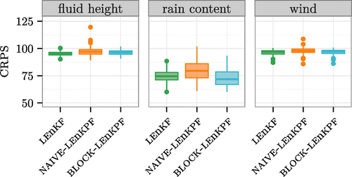
The relatively less good performance of the NAIVE-LEnKPF compared to the BLOCK-LEnKPF in this scenario might come from the added discontinuities in the analysis. In the high-frequency scenario the problem was not apparent as the system only evolved for a short time before new observations were assimilated. With low-frequency observations, however, the discontinuities introduced by the NAIVE-LEnKPF have more time to produce a detrimental effect on the dynamical evolution of the system, which results in a poorer performance.
5. Summary and discussion
We introduced two new localized algorithms based on the EnKPF in order to address the problem of non-linear and non-Gaussian data assimilation, which is becoming increasingly relevant in large-scale applications with higher resolution. The algorithms that we propose combine the EnKF with the PF in a way that avoids sample degeneracy. We took particular care to localize the analysis without introducing harmful discontinuities, which is an inherent problem of local PFs.
The results of the numerical experiments with a modified SWEQ model confirm that the proposed algorithms are promising candidates for application to convective scale data assimilation problems and have some distinct advantages compared to the LEnKF. The two local EnKPFs provide better estimates of the rain field, which has non-Gaussian characteristics and thus benefits greatly from the PF component of the algorithms. This advantage is the strongest either in the high-frequency scenario for short assimilation periods, or in the low-frequency scenario on longer time scales for the BLOCK-LEnKPF. Calibration is not perfect as can be seen from the rank histograms, but the improvements in CRPS indicate that the new algorithms are better in terms of sharpness while keeping calibration the same. In general the NAIVE-LEnKPF performs a little worse than the BLOCK-LEnKPF, but it is more straightforward to implement and might thus be suitable for large-scale applications.
Assimilating high-frequency observations over long periods of time seems to be problematic for all algorithms, as they grow overconfident and are not able to adapt when new clouds appear in the field. Indeed, if one does not assimilate other types of observations the filter is not able to correctly capture the unobserved fluid height field before it produces rain and performances deteriorate quickly after an initial improvement. It is not certain if such a behaviour is particular to the present SWEQ model or if it is an inherent characteristic of convective scale assimilation, but it indicates some potential limits of such scenarios. One possible path to tackle this issue would be to properly account for model error. Indeed, the present case study is not a perfect model experiment, as we assume that the observations are linear and Gaussians where in fact they are not. The typical approach to account for model error is to inflate the covariance, but there is a lot of research to do to understand how to apply such ideas in the context of PF like algorithms.
In many applications, the use of a square-root filter such as the LETKF has been shown to be of great benefit. Therefore, we are currently investigating possibilities to reformulate the EnKPF in this framework. In order to study the impact of localization on the quality of the analysis, we applied the two new localized EnKPFs to some simpler set-ups than in the present paper, where it is possible to analyse more closely the problem of discontinuities (Robert and Künsch, Citation2016). Given the promising results of the localized EnKPFs, we are collaborating with Meteoswiss and Deutscher Wetterdienst on adapting our algorithms to cosmo, a convective scale, non-hydrostatic NWP model.
Disclosure statement
No potential conflict of interest was reported by the authors.
Acknowledgements
We are very thankful to Daniel Leuenberger from Meteoswiss for fruitful discussions and comments, to Michael Würsch for his support for implementing and interpreting his modified SWEQ model, and to the reviewers for their valuable comments.
Notes
The underlying research materials for this article can be accessed at https://github.com/robertsy/assimilr.
Related Research Data
References
- Ades, M. and van Leeuwen, P. J. 2013. An exploration of the equivalent weights particle filter. Q. J. Roy. Meteorol. Soc. 139(672), 820–840.
- Alspach, D. L. and Sorenson, H. W. 1972. Nonlinear Bayesian estimation using Gaussian sum approximations. IEEE Trans. Autom. Control 17(4), 439–448.
- Bauer, P., Thorpe, A. and Brunet, G. 2015. The quiet revolution of numerical weather prediction. Nature 525(7567), 47–55.
- Bengtsson, T., Snyder, C. and Nychka, D. 2003. Toward a nonlinear ensemble filter for high-dimensional systems. J. Geophys. Res. Atmos. 108(D24). Online at: http://onlinelibrary.wiley.com/doi/10.1029/2002JD002900/full
- Carpenter, J., Clifford, P. and Fearnhead, P. 1999. Improved particle filter for nonlinear problems. IEE Proc. Radar Sonar Navig. 146(1), 2–7.
- Crisan, D. 2001. Particle filters – A theoretical perspective. In: Sequential Monte Carlo Methods in Practice (eds. A. Doucet, N. D. Freitas and N. Gordon), Statistics for Engineering and Information Science. Springer, New York, pp. 17–41.
- Doucet, A., De Freitas, N. and Gordon, N. 2001. Sequential Monte Carlo Methods in Practice. Springer, New York.
- Evensen, G. 1994. Sequential data assimilation with a nonlinear quasi-geostrophic model using Monte Carlo methods to forecast error statistics. J. Geophys. Res. Oceans 99(C5), 10143–10162.
- Evensen, G. 2009. Data Assimilation: The Ensemble Kalman Filter. Springer, New York.
- Frei, M. and Künsch, H. R. 2013. Bridging the ensemble Kalman and particle filters. Biometrika 100(4), 781–800.
- Gaspari, G. and Cohn, S. E. 1999. Construction of correlation functions in two and three dimensions. Q. J. Roy. Meteorol. Soc. 125(554), 723–757.
- Gneiting, T. and Katzfuss, M. 2014. Probabilistic forecasting. Ann. Rev. Stat. Appl. 1(1), 125–151.
- Gneiting, T. and Raftery, A. E. 2007. Strictly proper scoring rules, prediction, and estimation. J. Am. Stat. Assoc. 102(477), 359–378.
- Gordon, N., Salmond, D. and Smith, A. 1993. Novel approach to nonlinear non-Gaussian Bayesian state estimation. IEE Proc. F Radar Signal Process. 140(2), 107–113.
- Hamill, T. M., Whitaker, J. S. and Snyder, C. 2001. Distance-dependent filtering of background error covariance estimates in an ensemble Kalman filter. Mon. Weather Rev. 129(11), 2776–2790.
- Haslehner, M., Janjić, T. and Craig, G. C. 2016. Testing particle filters on simple convective-scale models Part 2: A modified shallow-water model. Q. J. Roy. Meteorol. Soc. 142(697), 1628–1646.
- Houtekamer, P. L. and Mitchell, H. L. 1998. Data assimilation using an ensemble Kalman filter technique. Mon. Weather Rev. 126(3), 796–811.
- Houtekamer, P. L. and Mitchell, H. L. 2001. A sequential ensemble Kalman filter for atmospheric data assimilation. Mon. Weather Rev. 129(1), 123–137.
- Hunt, B. R., Kostelich, E. J. and Szunyogh, I. 2007. Efficient data assimilation for spatiotemporal chaos: A local ensemble transform Kalman filter. Physica D 230(1–2), 112–126.
- Kalman, R. E. 1960. A new approach to linear filtering and prediction problems. J. Basic Eng. 82(1), 35–45.
- Kalman, R. E. and Bucy, R. S. 1961. New results in linear filtering and prediction theory. J. Basic Eng. 83(1), 95–108.
- Künsch, H. R. 2005. Recursive Monte Carlo filters: Algorithms and theoretical analysis. Ann. Stat. 33(5), 1983–2021.
- van Leeuwen, P. J. 2009. Particle filtering in geophysical systems. Mon. Weather Rev. 137(12), 4089–4114.
- van Leeuwen, P. J. 2010. Nonlinear data assimilation in geosciences: An extremely efficient particle filter. Q. J. Roy. Meteorol. Soc. 136(653), 1991–1999.
- Lei, J. and Bickel, P. 2011. A moment matching ensemble filter for nonlinear non-Gaussian data assimilation. Mon. Weather Rev. 139(12), 3964–3973.
- Liu, J. S. 1996. Metropolized independent sampling with comparisons to rejection sampling and importance sampling. Stat. Comput. 6(2), 113–119.
- Lorenz, E. N. and Emanuel, K. A. 1998. Optimal sites for supplementary weather observations: Simulation with a small model. J. Atmos. Sci. 55(3), 399–414.
- Musso, C., Oudjane, N. and Le Gland, F. 2001. Improving regularised particle filters. In: Sequential Monte Carlo Methods in Practice (eds. A. Doucet, N. De Freitas and N. Gordon). Springer, New York, pp. 247–271.
- Nakano, S. 2014. Hybrid algorithm of ensemble transform and importance sampling for assimilation of non-Gaussian observations. Tellus A 66, 21429.
- Ott, E., Hunt, B. R., Szunyogh, I., Zimin, A. V., Kostelich, E. J., co-authors. 2004. A local ensemble Kalman filter for atmospheric data assimilation. Tellus A 56(5), 415–428.
- Papadakis, N., Memin, E., Cuzol, A. and Gengembre, N. 2010. Data assimilation with the weighted ensemble Kalman filter. Tellus A 62A, 673–697.
- Pitt, M. K. and Shephard, N. 1999. Filtering via simulation: Auxiliary particle filters. J. Am. Stat. Assoc. 94(446), 590–599.
- Poterjoy, J. 2016. A localized particle filter for high-dimensional nonlinear systems. Mon. Weather Rev. 144(1), 59–76.
- Reich, S. 2013. A guided sequential Monte Carlo method for the assimilation of data into stochastic dynamical systems. In: Recent Trends in Dynamical Systems (eds. A. Johann, H.-P. Kruse, F. Rupp and S. Schmitz), Vol. 35, Springer Proceedings in Mathematics & Statistics. Springer, Basel, pp. 205–220.
- Robert, S. and Künsch, H. R. 2016. Localization in high-dimensional Monte Carlo filtering. ArXiv:1610.03701.
- Sigrist, F., Künsch, H. R. and Stahel, W. A. 2012. A dynamic nonstationary spatio-temporal model for short term prediction of precipitation. Ann. Appl. Stat. 6(4), 1452–1477.
- Snyder, C., Bengtsson, T., Bickel, P. and Anderson, J. 2008. Obstacles to high-dimensional particle filtering. Mon. Weather Rev. 136(12), 4629–4640.
- Snyder, C., Bengtsson, T. and Morzfeld, M. 2015. Performance bounds for particle filters using the optimal proposal. Mon. Weather Rev. 143(11), 4750–4761.
- Stidd, C. K. 1973. Estimating the precipitation climate. Water Resour. Res. 9(5), 1235–1241.
- Würsch, M. 2014. Testing data assimilation methods in idealized models of moist atmospheric convection. Ph.D. thesis, Ludwig-Maximilians-Universität München.
- Würsch, M. and Craig, G. C. 2014. A simple dynamical model of cumulus convection for data assimilation research. Meteorol. Z. 23(5), 483–490.
Appendix 1
Details for BLOCK-LEnKPF
Using the factorization (Equation11(11) ) and
, Bayes’ rule gives the following factorization of the analysis distribution
(A1)
where
By integrating out , we obtain
(A2)
The last step can be easily checked by integrating out and
, respectively. The posterior of
is nothing else than the prior, which comes as no surprise because
is independent from
and thus is not influenced by
. Also, independence between
and
continues to hold.
Finally, the conditional posterior of can be derived from the definition of conditional probability
(A3)
where we see that all the terms involving cancel out. Therefore the conditional posterior of
is nothing else than the conditional prior distribution.
Assuming additionally that is normal, the conditional distribution of
is again normal with the following mean and covariance:
(A4)
(A5)
where(A6)
However, instead of making a new random draw from this conditional normal distribution, one can instead devise a method which reuses the background samples. Again under the Gaussian assumption, the residual(A7)
is independent of and
and normally distributed with mean 0 and covariance
. Hence we can use this residual for sampling from the conditional distribution
:
(A8)
because . Plugging in the definition of
we obtain the analysis of Equation (Equation12
(12) ).
In order to understand better how the BLOCK-LEnKPF works, let us compare it to the EnKPF analysis of the entire state using the block
and not assuming the factorization Equation (Equation11
(11) ). Applying the definitions Equations (Equation10
(10) ) and (Equation8
(8) ) in the case where
and H have the block structure
(A9)
and(A10)
it can be easily verified that(A11)
and(A12)
Therefore(A13)
(A14)
and(A15)
Moreover and
. Combining these results with Equation (Equation6
(6) ), we obtain the following for the analysis of
with a full EnKPF:
(A16)
Therefore the BLOCK-LEnKPF update given by Equation (Equation12(12) ) is the same as the EnKPF update given by Equation (EquationA16
(A16) ) for those indices where
. However, for indices i with
, the EnKPF analysis applies a correction to
and not to
and the size of the correction depends on
and not on
. Moreover
is replaced by
which is in conflict with the requirement of a local analysis. Applying a correction to
while setting
would introduce a discontinuity between
and
. Therefore if
, we do not apply an EnKPF analysis to
, but use instead Equation (Equation12
(12) ), ensuring a smooth transition between
and
. If
and
are only uncorrelated, but not independent, we ignore some higher order dependence between these values by pairing
with
in cases where
, but this seems unavoidable.