Scale-dependent estimates of the growth of forecast uncertainties in a global prediction system

Abstract

We assess the scale-dependent growth of forecast errors based on a 50-member global forecast ensemble from the European Centre for Medium Range Weather Forecasts. Simulated forecast errors are decomposed into scales and a new parametric model for the representation of the error growth is applied independently to every zonal wavenumber. In contrast to the standard fitting method, the new fitting function involves no time derivatives and provides the asymptotic values of the forecast errors as a function of the fitting parameters. The range of useful prediction skill, estimated as a scale where forecast errors exceed 60% of their asymptotic values is around 7 days on large scales and 2–3 days at 1000 km scale. The new model is easily transformed to the widely used model of Dalcher and Kalnay (1987) to discuss the scale-dependent growth as a sum of two terms, the so-called and terms. Their comparison shows that at planetary scales their contributions to the growth in the first two days are similar whereas at small scales the term describes most of a rapid exponential growth of errors towards saturation.

Keywords:

• forecast errors
• error growth
• parametric models
• prediction limits
• scale dependency

1. Introduction

The representation of the growth of forecast errors by simple parametric models has a long tradition in numerical weather prediction (NWP). The first of such models was introduced by Leith (1978). His two-parameter model described the forecast error variance V as a function of the forecast range t:(1) Leith (1978) interpreted the two parameters of (1(1) ) as describing the inherent error growth from imperfect initial conditions (term ) and the model error source term due to the imperfect representation of the atmosphere (term S) by an NWP model. The solution of (1(1) ) as a function of initial state error variance V(0) can be written as . As in many follow-on studies (e.g. Leith, 1978; Dalcher and Kalnay, 1987; Savijärvi, 1995) the errors V(t) were here obtained by comparing forecasts of the geopotential height of 500 hPa level with analyses that served as initial conditions for the forecasts and therefore .

Since the model (1(1) ) did not allow for the saturation of forecast error variances, it was not suitable beyond the first few days of forecasts. A more well-known model was proposed by Lorenz (1982) to describe the growth of root-mean-square (r.m.s.) errors E(t) towards saturation:(2)

The right-hand-side of Equation (2(2) ) parametrizes the slow growth of errors towards asymptotic (saturation) value at long forecast times. The solution of (2(2) ) is a function of the initial state r.m.s. error E(0), the exponential growth rate and the asymptotic error , and can be written as: . Notice that .

In Lorenz (1982) and several subsequent studies (e.g. Simmons et al., 1995), E(t) were measured by the growth ofdifferences between forecasts started one day apart. This approach provides somewhat different estimates of E(t) than if the forecast errors are computed from differences between forecasts and analyses. Due to its assumption of ’perfect model’, the former approach better suits the model (2(2) ) which neglected the growth due to model errors and which best applies to the regime with (Lorenz, 1996). However, it has proved difficult to accurately represent short-range errors that are characterized by a more linear growth (e.g. Simmons and Hollingsworth, 2002).

An extended model that takes into account both the slow error growth close to saturation and a linear component of the growth was introduced by Dalcher and Kalnay (1987):(3)

This three-parameter model combines (1(1) ) and (2(2) ) and it has been widely used to describe the error growth rate proportional to the amount by which the errors fall short of saturation. The analytical solution of (3(3) ) is , where .

Neither this complicated solution nor less complex solutions of (1(1) )–(2(2) ) have been fitted to data directly. Instead, the three parameters of (3(3) ) are estimated from the data by evaluating against E as:(4)

Time step is usually one day, , with being the error at day i. The parameters , and are determined by a least-squares fit of the values of and that are given by r.m.s. difference between forecasts and analyses or between forecasts with ranges i and days, verifying on the same day (Simmons and Hollingsworth, 2002). Unless assuming that , this approach needs an independent estimate of the initial error E(0). The asymptotic value can also be independently obtained as the average r.m.s. difference between independent analyses leaving for fitting only two parameters (Bengtsson et al., 2008).

Dalcher and Kalnay (1987) and subsequently Reynolds et al. (1994) applied (3(3) ) for the forecast-error variances V(t) rather than their r.m.s. values E(t). They also adopted letter S as used by Leith (1978) to denote the error growth due to model deficiencies. However, the majority of recent studies adopted Greek letter which is why we have chosen it in (3(3) ). For the same reason we in (3(3) ) wrote E (rather than V) as we shall be dealing with the statistics of r.m.s. errors. We also note that Simmons and Hollingsworth (2002) wrote (3(3) ) as . They argued that a linear term in this error-growth equation (i.e. term in (4(4) )) represents also a part of the growth of analysis errors that is more rapid during the first 1–2 days of the forecasts than further into the forecast range, and is not necessarily associated with model error. The assumption of the linear growth component associated with the model deficiencies has been argued in several studies (e.g. Reynolds et al., 1994; Kuhl et al., 2007), especially in the tropics where parametrization of deep convection leads to large errors early in the forecasts.

The least-square fit of (4(4) ) has traditionally been performed for the r.m.s. errors of the geopotential height at 500 hPa level in extratropics. Such a recent study by Magnusson and Källén (2013) suggested that the contribution to the error growth in the forecasting system of the European Centre for Medium Range Weather Forecasts (ECMWF) at short lead times is of the same order of magnitude for the term and for the term of (3(3) ). They also estimated to be around 110 days since 2000. Herrera et al. (2016) fitted the THORPEX Interactive Grand Global Ensemble data from the four operational ensemble prediction systems (ENS) (ECMWF, NCEP, JMA and CMC) to (4(4) ) and compared the estimates of and parameters for the 500 hPa geopotential height variable. They reported relatively similar values of (around 0.3–0.5 per day) for various ensemble systems but largely different values for .

Geopotential height field at 500 hPa is dominated by large-scale features and quasi-geostrophic balance which is well analysed by data assimilation schemes (e.g. Park et al., 2008). Small scales which tend to grow at a faster rate than the larger scales of motions, have little variance at 500 hPa. It is thus interesting to provide a picture of the forecast errors growth as a function of scale from the initial uncertainties simulated by the operational ENSs. An example of such evaluation was carried out by Simmons (2006) who presented the spectra of mean-square errors for geopotential height, temperature and vorticity for the ECMWF model. His analysis showed that over the last decade the errors have become more uniformly distributed across the spectrum in contrast to 1980–1990 period which was characterized by significant errors in the largest synoptic scales. Simmons (2006) discussed two timescales for the growth of errors in smaller spatial scales: a rapid growth and an apparent saturation early in the forecast range and a slowly evolving component of error throughout the forecast range. Harlem et al. (2005) noted two distinct broad regimes of the error growth in vorticity field at 500 hPa, the initial fast growth with E well below and the other with larger E.

The present paper extends these studies by providing a scale-dependent estimates of the growth of forecast errors and limits of useful prediction skill based on the forecast-uncertainty statistics of both geopotential and wind field simulated by the operational ENS of ECMWF. We perform the decomposition of simulated forecast errors into scales and estimate the time scale of useful prediction skill as a function of the zonal wavenumber. For this purpose, we developed a new model for the parametrization of the growth of forecast errors. Its solution, given by tangent hyperbolic functions, is simpler than the solutions of (1(1) )–(3(3) ) and it provides a more accurate fit to data than the fit of and according to (4(4) ). The new model is used to compute the and parameters of (3(3) ) across many scales and interpret them in relation to dynamics.

The paper consists of five sections. In Section 2 we introduce the operational ENS of ECMWF and the method for the scale-dependent decomposition of the ensemble data on terrain-following levels. In Section 3 we present a new function to fit the empirical data and its relation to the model (3(3) ). Section 4 contains results and finally conclusions are given in Section 5.

2. Scale-dependent forecast-error statistics

We use standard deviation between ensemble members (usually referred to as ensemble spread) from the ECMWF ENS, as a proxy of global forecast errors. The application of the ENSs for the estimation of analysis and forecast uncertainties has become common in recent years. For example, Buizza and Leutbecher (2015) used the ECMWF ensemble forecasts to estimate the scale of useful prediction for instantaneous, grid-point fields between 16 and 23 days. Žagar et al. (2015a) showed that analysis uncertainties in the ECMWF ensemble are largest on large scales in the tropics. They also showed that the curves of the growth of forecast uncertainties measured by the standard deviation of the forecast ensemble (i.e. the ensemble spread) follow fairly well the curves of the r.m.s. differences between the ensemble mean and the control analysis (i.e. forecast errors). This suggests that the ensemble spread can be used as a proxy for the forecast-error statistics. ENSs also provide statistics of the initial uncertainties that have not been considered in most of earlier studies of the limits of prediction skill in NWP models.

The advantage to use the ensemble spread to test an error growth model is to have a number of realizations each day, which gives less noisy statistics compared to the use of real forecast errors. The primary data-set used here consists of 2 weeks of data of 15-day long ensemble forecasts from May 2015. The properties of this data-set are compared to a data-set from December 2014 from the same ensemble system. December data-set consists of 31 forecast days but with a limitation of 7-day forecast length. The latter data-set was used by Žagar et al. (2015a, hereafter ŽBT). In this section we briefly describe the data and outline the method used to decompose the data into scales. This is followed by a discussion of basic properties of the error growth in two data-sets.

Properties of the ECMWF ensemble system are described in many papers, for example Buizza and Leutbecher (2015), Isaksen et al. (2010) and Buizza et al. (2008). Initial state perturbations for the ensemble are a combination of perturbations from an ensemble of analyses produced by 4D-Var data assimilation (Isaksen et al., 2010) and singular vectors (Buizza et al., 2008). The singular vectors are constructed to maximize the perturbation growth in wavenumbers 1–42 over the first 48 h. The model uncertainties are simulated using two model error schemes, the Stochastically Perturbed Parameterized Tendency scheme (SPPT, Buizza et al., 1999; Palmer et al., 2009) and the Stochastic Kinetic Energy Backscatter scheme (SKEB, Shutts, 2005; Palmer et al., 2009) scheme. SPPT is designed to simulate random model errors due to parameterized physical processes. For every grid point column, the sum of the physical tendencies is perturbed by a scaling factor which comes from a pattern generator. The effective scales of the perturbations are a combination of the length scales in the pattern generator and the scales of the physical processes. SKEB is designed to simulate the upscale energy transfer and the perturbed scales are wavenumbers 1–159.

The ECMWF ENS data are produced with a variable resolution which at the time of production of these data-sets were a horizontal resolution T639 during the first 10 days and T319 (i.e. about 65 km spacing) thereafter. The operational ensemble includes 50 members and a control simulation, run from the unperturbed analysis and without model error schemes. The vertical discretization for ENS is 91 hybrid vertical levels. In this study we utilize the model-level data on the N64 regular Gaussian grid ( points). The top model levels which are known to show some permanent error structures are not used; concretely, we analysed 73 model levels between the surface and 10 hPa. The applied data are from 00 UTC run and the outputs were available every 12 h including the initial time that makes 31 samples on the temporal axis for May 2015 data-set and 15 samples for the 7-day long forecasts in December 2014.

The data are decomposed in scales using the method of ŽBT that relies on the projection of the global dynamical fields in terms of the 3D orthogonal normal-mode functions (NMFs). The representation consists of the vertical decomposition of the baroclinic atmosphere in terms of M global shallow-water systems and a projection of horizontal motions for every vertical mode. Each shallow-water system is characterized by average fluid depth, known as the equivalent depth. The maximal M is equal to the number of model levels. The horizontal motions for a given vertical mode are represented by a series of Hough harmonics that consist of the Hough vector functions in the meridional direction and waves in the longitudinal direction. The meridional modes include the balanced (or Rossby) modes and eastward-propagating and westward-propagating inertio-gravity (or unbalanced) modes. The inertio-gravity and Rossby modes are eigensolutions of the linearized primitive equations and they are known as oscillations of the first and second kind, respectively (e.g. Kasahara, 1976). The details of the projection procedure are available in Žagar et al. (2015b) and references therein.

A discrete solution is obtained by using the truncated Fourier series in the zonal direction and a finite number of the Hough vectors in the meridional direction. The truncations are defined based on the data resolution. We selected 120 zonal wavenumbers and 180 meridional modes which include Rossby and inertio-gravity components of the Hough vector functions. In the vertical direction, we used modes. This provides a representation of the geopotential height field, surface pressure field and winds in terms of the complex coefficients , with indices k, n and m representing the zonal wavenumber (k), the meridional mode (n) and the vertical mode (m) index. The ensemble spread is obtained by computing the standard deviation of the 50-member ensemble in the modal space for 12-hourly outputs of 15 and 7 days long forecasts for May 2015 and December 2014, respectively. As in ŽBT, the ensemble spread is denoted . The error statistics is obtained by averaging the data at each time step of forecasts over all samples.

The 3D orthogonality of the NMF representation allows us to integrate the scale-dependent spread along any of the three spatial directions (k, n, m). In the present paper we focus to the zonal wavenumber index. For every k at every time step, we integrate the spread across all meridional and vertical scales and for all Hough modes (Rossby and inertio-gravity modes) and discuss dynamics of over the forecast range. As shown in ŽBT, the computation of the squared ensemble spread (ensemble variance) in modal space is equivalent to the variance computed in physical space for the two wind components and geopotential height normalized by the equivalent fluid depth for the 3D baroclinic model atmosphere represented in terms of M shallow-water layers:(5)

Here, , and denote departures of the ensemble member p from the ensemble mean for wind components and geopotential height at location . The summations in physical space is with respect to the zonal index i and meridional index j of the horizontal grids of the mth shallow-layer after the vertical data transform. Each vertical mode is characterized by its equivalent depth . Parameter g stands for gravity and the size of ensemble is . The unit of the spread is . The complete derivation is presented in ŽBT.

Figure 1. Growth of the global forecast errors simulated by the ECMWF ensemble forecasting system in (a) 7-day forecasts in December 2014 and (b) 15-day forecasts in May 2015. Presented quantity is defined by Equation (6(6) ) as a function of the zonal scale L which is defined as (km), where k is the zonal wavenumber. The zonal (x) axis is logarithmic and the meridional axis (time) is linear.

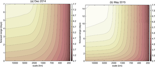
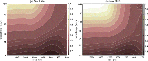
Figure 2. As in Fig. 1 but the errors are normalized with their values at initial time in the same scale. Presented quantity is . Notice that y axis is also logarithmic in order to show more clear the relative growth early in forecasts.

The scale-dependent statistics of the forecast-error growth, which is denoted E(k, t) is defined as(6)

and it represents the global meridionally and vertically integrated errors at time step t simulated by the ENS. For simplicity, in the rest of the paper we shall refer to the quantity E(k, t) as forecast errors. In addition to E(k, t) we use the normalized forecast errors which we denote F(k, t) and define as:(7)

In addition to discussing all scales, we consider integrated errors in the planetary, synoptic and subsynoptic scales. Wavenumbers belonging to the three scale ranges are defined following Jung and Leutbecher (2008): the zonal wavenumbers represent the planetary scales, wavenumbers represent the synoptic scales whereas all belong to the subsynoptic scales. The normalized errors are defined as(8)

for the planetary (denoted ), synoptic (denoted ) and subsynoptic (or mesoscale, denoted ) scale range, respectively. In the mid-latitudes, the zonal scales under 1000 km thus belong to the subsynoptic range whereas in the tropics the subsynoptic range starts at around 1300 km. Note that the ensemble spread in (6(6) ) is multiplied by the square root of two when used as a proxy for the forecast errors.

In Fig. 1 we present the simulated r.m.s. errors E(k, t) defined by (6(6) ) for the two data periods. The growth of the global forecast errors is presented as a function of the zonal scale L defined at the equator as , where is the zonal wavenumber and  km is the average Earth radius. In Fig. 2, the errors are normalized by their initial values in each k to show a relative growth as a function of scale. Notice that Fig. 1 uses a linear y-axis whereas Fig. 2 has been drawn using a logarithmic y-axis to better visualize the growth in early stages of the forecasts and therefore the initial () time is not shown.

Figure 1 shows much larger magnitudes of simulated errors in the synoptic and planetary scales than in subsynoptic scales. This is in contrast to the traditional view of initial errors in small scales and their upscale cascade. In global NWP and ensemble systems, there are significant analysis uncertainties at large scales and large initial perturbations at largest scales, especially in the tropics (ŽBT). These perturbations grow from the start of the forecast in all scales as discussed in ŽBT. The growth in small scales quickly leads to saturation and after 2 days scales under 1000 km appear to be saturated. The clear discontinuity at day 10 in subsynoptic scales in Fig. 1(b) is related to the change of the horizontal resolution of the ensemble as described above.

We do not notice a significant difference between the data for December and May in Fig. 1. Some difference can be noticed in the relative growth in Fig. 2. The error growth in baroclinic scales is larger in the northern hemisphere extratropical winter than in summer. This is seen in Fig. 2(a) as a minimum in scales between 2500 and 5000 km. The corresponding zonal wavenumbers are 4–6. This feature of the global data-set is similar to that found in the error statistics at 500 hPa geopotential height in winter.

The smallest growth relative to E(k, 0) is centred around 700 km in both data-sets suggesting that it is a property of the ensemble system. While we do not know the exact reasons, a plausible explanation is the use of singular vectors that maximizes the growth for scales longer than wavenumber 42 during the first 2 days, and do not include the subsynoptc scales. We can also notice in Fig. 2 that the minimum of the relative error growth shifts towards smaller scales during the first 2–3 days of the forecasts until subsynoptic scales become saturated. In 15-day forecast range, E(k, t) increases between eight times in the planetary scales and up to twice in mesoscale relative to E(k, 0).

Studies addressing dependence of forecast error growth on horizontal scale are rare. Such evaluation was carried out by the mentioned study of Simmons (2006) who differentiated between a rapid growth and a quick saturation of errors in small scales and a slowly evolving component of error afterward. The former is likely a result of intrinsic dynamics with small temporal as well as spatial scales whereas the latter may be directly forced by large-scale dynamical and thermodynamical processes that have much slower intrinsic error growth rates. This forcing of small-scale errors by larger mesoscale and synoptic scales processes may be the reason for the apparent shifts towards smaller scales during the first 2–3 days in Fig. 2. As the two data-sets show very similar properties, the results will be presented for the May 2015 data-set which is longer. We shall discuss the shorter data-set to show that the function fitting can be successfully applied also to shorted forecasts.

3. Modelling of the growth of forecast errors

In this section we present a new model for the growth of forecast errors. First we derive a model that describes dynamics of forecast errors E(k, t). This is followed by a presentation of a closely related model for the growth of normalized errors F(k, t). As the spatial scale is not a parameter of the model, we drop k for the rest of this section and denote errors in ms and normalized errors without units by E(t) and F(t), respectively.

3.1. Function fitting for the growth of forecast errors

The new function to fit the the evolution of the forecast errors E(t) has the following form:(9)

where (a, b) and (A, B) are pairs of parameters linearly transforming the argument of the hyperbolic tangent and its value, respectively. In Appendix 1 we show that this model is equivalent to the logistic function, but it is simpler to apply in fitting procedures and numerically better behaved (see below).

By taking the time-derivative of the model function E(t) and expressing time t as a function of E, we can write the derivative solely as a function of E. Thereby we obtain an autonomous ordinary differential equation(10)

where parameter s is defined as . As we are fitting real valued data, we have two choices for the parameters

The second choice gives a non-realistic singularity at and therefore we work with first choice, where all the parameters are real numbers. Additionally, due to nature of the error this can only increase in time so that we request . This represents a constraint on two parameters: . Without the loss of generality we choose . Consequently, we can write the maximal and minimal values of the model function as(11)

By using (11(11) ), we rewrite Equation (10(10) ) as(12)

where it is clear that . Note, that the right-hand side of this equation is a real second degree polynomial with real roots and a positive coefficient in front of the leading term. There are no additional mathematical constraints. Nevertheless, because the forecast errors are always positive and monotonically increasing, we introduce additional constraints on the parameters, reading

that sets the lower limit to B as . We should remember that by definition .

The ordinary differential Equation (12(12) ) has three parameters and those are connected to the parameters of fitting function (a, b, A, B) as(13)

whereas the initial condition , determines the fourth parameter, b, as(14)

According to differential equation (12(12) ), the forecast error is autonomous and fully determined by its initial value. Due to simplicity of the model, the forecast error growth curves are also self-similar. The autonomy and self-similarity of the error growth is a property of simplified dynamical systems applicable to atmospheric dynamics (e.g. Düben et al., 2014).

3.2. Fitting the growth of normalized errors

If we focus on normalized errors for which (as visualized in Fig. 2), Equation (9(9) ) transforms to the following function:(15)

where F(t) represents normalized error data, and a, b, c are real constants to be determined by the fitting procedure. By definition a and c are positive, whereas b can have an arbitrary sign. Because F(t) has only three parameters it is better behaved in fitting than E(t) defined by (9(9) ).

The function F(t) has two distinguished limits: its asymptotic or saturation value and its minimal value , that are given by(16)

and(17)

The latter is only of theoretical interest here and should not be interpreted as the initial error. Note that the exponential growth rate a in (15(15) ) of the chaotic internal growth does not appear in the expression for the asymptotic error in (16(16) ). Note also that .

By inserting into Equation (12(12) ) we obtain an ordinary differential equation for F(t), written as(18)

Consequently, by knowing initial error E(0) we can easily transform Equation (18(18) ) describing normalized error F(t) and parametrized by into Equation (12(12) ) describing absolute error E(t):(19)

Furthermore, we can use the initial error E(0) and the parameters (b, c) of Equation (15(15) ) to express the parameters (A, B) of the basic model (9(9) ) as(20)

Other two parameters, a and b, do not change between the models.

As the error approaches its asymptotic value , the curve F(t) can be approximated by the following exponential behaviour:(21)

We can define the time scale when becomes a good approximation of F(t) by requesting their difference to be within a certain limit of . By comparing (15(15) ) and (21(21) ) and using (16(16) ) we can write F(t)

The leading order of the difference between (15(15) ) and (21(21) ) is

We request to be within 10% of , i.e. , , that leads to the expression for the time scale when the asymptotic error dynamics is well described by the exponential form (21(21) ) (after the initial phase with the fast growth):(22)

3.3. Relationship with the model of Dalcher and Kalnay (1987)

The three parameters of the model (3(3) ) by Dalcher and Kalnay (1987) can be easily computed from the parameters of the models (18(18) ) or (12(12) ). The asymptotic value is obtained from Equation (20(20) ) after and are calculated by (16(16) )–(17(17) ). The exponential growth rate and the parameters can be written in terms of the parameters of model (12(12) ) as(23)

or in terms of the parameters of the model (18(18) ) for the normalized error growth as(24)

Units of a and are the same, one over time unit. Parameters b and c are non-dimensional and the unit of is equal to the unit of E divided by the time unit. The units of A and B are the same as the unit of E. In our case, E is in m/s and for the time unit we shall use day as usual in applications of (3(3) ).

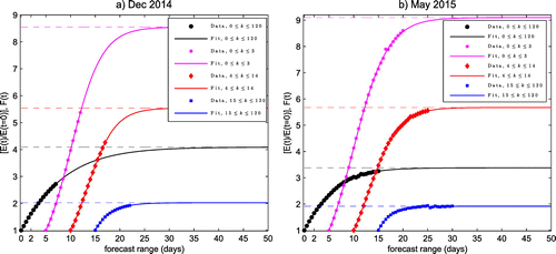
Figure 3. Function fitting of the normalized error growth in different scales in (a) December 2014 and (b) May 2015. Empirical data are presented by markers and their fit based on Equation (9(9) ) by full lines. The data and fitting solutions for planetary scales () is shifted along the x-axis for 5 days, synoptic scales () are shifted for 10 and subsynoptic scales () for 15 days along the x axis. Dashed lines correspond to the asymptotic values of the normalized forecast errors as defined by Equation (16(16) ).

With the signs of all parameters fixed, it is clear that . The sign of in principle depends on the sign of (or ) and is fixed by known constraints. Numerical results show that for our data and consequently .

3.4. Application of the new model to ECMWF data

The application of the new model to the ECMWF ensemble forecasts involves three steps. First, the 50-member ensembles of forecasts are decomposed into scales and the ensemble spread is computed for every forecast time followed by averaging over all samples. This provides errors E(k, t) and normalized errors F(k, t) defined by (6(6) ) and (7(7) ), respectively. Then the function is fitted to the normalized errors F(t) for each wavenumber k by the least-square fit using Wolfram Mathematica, which minimizes the difference between the fitting function and data. The least-square minimization, in order to obtain optimal parameters (a, b, c), is performed by the Levenberg–Marquardt algorithm. The fitting is carried out also for , , and for the total F integrated over all k. For small scales (), which show to saturate very fast, the fitting was compared for several methods: Levenberg–Marquardt, Newton, conjugate gradient method and numerical minimization. In the third step, the three parameters of (3(3) ) are computed for the comparison with previous studies. First the asymptotic values are obtained from (16(16) ,17(17) ), then and are calculated from (24(24) ).

4. Results

4.1. Fitting the scale-dependent growth of forecast errors in ECMWF system

First we show results of fitting the normalized error data for the three ranges of spatial scales and for all scales together (total global errors). Please note that the curves for the different scales are staged by 5 days on the x-axis in the plots. Figure 3 presents results for both 15-day forecast range in May 2015 and for 7-day long period in December 2014. Solutions for the functions F(t) are shown as curves on top of the data. The discrepancy between the model and the data is quantified by evaluating the mean square difference between the data points and the model fit. The model fits the data in all cases very well over the whole time interval, with values of average squared difference of the order to . For comparison, the data fitting by the standard approach (4(4) ) produces errors – (not shown). The only data points somewhat off the fitting curves in Fig. 3 are in the subsynoptic regime after forecast day 10 due to the resolution change (Fig. 3(b)). It appears that the change of resolution stops the slow growth of the spread in mesoscale at day 10 so that in this range we performed the fitting for the 10-day data.

Dashed horizontal lines in Fig. 3 represent the asymptotic values for the simulated forecast errors as multipliers of the initial error. From these values one could in principle infer the error doubling time for various scales. However, the error-doubling time varies for different variables, different scales and NWP models (an overview is provided for example in Buizza and Leutbecher (2015)) and makes little sense for the global errors. Nevertheless, we notice that in the subsynoptic range, the errors do not double during the 15-day forecast range (), whereas it almost exactly doubled in December 2014 (). One interpretation here is that the initial errors are already in the saturation stage for short lead times. The parameter a, which represent the exponential growth rate of errors, is largest for the mesoscale range, as expected for atmospheric system (not shown). The asymptotic errors are related to the method for the generation of the mesoscale ensemble spread (i.e. simulation of the model uncertainty). This is reflected in (16(16) ) that presents as a function of the parameters b and c. A somewhat different time scale of the saturated subsynoptic errors in December and May months can result from many processes including different seasons and variability related to the active phase of ENSO in 2015 in addition to the shorter length of data in December 2014.

Figure 4. As in Fig. 3(b) but with the exponential solution (21(21) ) for the error dynamics near saturation added (red curves).

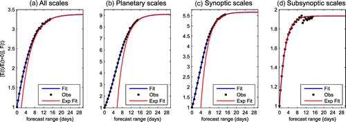
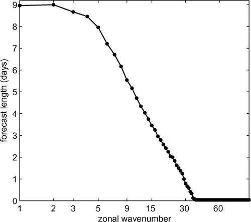
Figure 5. Forecast time when the difference between F(t) and becomes smaller than 10% of for each zonal wavenumber k. For F(t) is less than 10% different from from the beginning of forecasts.

The fact that subsynoptic errors are close to the saturation already for short lead times is further illustrated in Fig. 4. It shows solution of (21(21) ) for the asymptotic regime of the error growth close to saturation. The exponential growth solution denoted is added on top of the full solutions F(t) to illustrate how rapidly F(t) approaches to at different spatial scales. For the synoptic and planetary scales, it takes around a week to enter this regime whereas at the subsynoptic scales the two solutions appear very similar from the start. A more precise estimate of the transition time scale after which the growth slows down while exponentially approaching the saturation is shown in Fig. 5. Here, the criterion is evaluated for each wavenumber. The results confirm that for wavenumbers greater than 40, the magnitude of initial perturbations (i.e. ensemble spread) is smaller than 10% of their asymptotic errors. Thus, the asymptotic solution appears to be a good fit from the start of the forecast (Fig. 4d). It is possible that this result is at least partly associated with the formulation of initial perturbations in the ECMWF ensemble system and the cut-off scale for the application of singular vectors. Other explanation is that such rapid error growth is typical for three-dimensional turbulence (wavenumbers smaller than 40) that dominates smaller scale in contrast to more slow two-dimensional turbulence that dominates large scales and longer forecasts. We see in Fig. 5 that as the wavenumber increases, it takes longer for the errors to reach the asymptotic regime; at wavenumber 15 (scale around 1000 km in the mid-latitudes) it takes 3 days and for wavenumbers 5 and smaller it takes 8–9 days.

In planetary and synoptic scales the initial and asymptotic errors differ by a factor around 9 and 5.5–6, respectively (Fig. 3). The asymptotic level for the error integrated over all scales is about 3.5 times the initial error for the May data-set and about four times for the December data-set. The larger increase of errors in December than in May is in agreement with a larger variability in the northern hemispheric winter while the variability in the southern hemisphere is more constant over the year.

The ECMWF r.m.s. error for the 500 hPa geopotential height at day 15 in northern hemisphere is around 100 m in winter and 60 m in summer (Haiden et al., 2014). However, the geopotential height error at 500 hPa cannot be used alone for the comparison with our errors which include both mass and wind data. The growth of normalized forecast errors simulated by the ECMWF ensemble and fitted by the parametric model can be roughly compared to the growth estimated using standard verifications scores for dynamical variables in the models. For example, current analysis error for 500 hPa height is a couple of meters (Simmons, 2006). Forecast error at 1.5 days is around 10 m, at day 7, 50–60 m and at day 15 around 100 m (Haiden et al., 2014, data for winter 2013/2014). We also need to consider the growth of the wind-field errors which increase by a factor 2–3 between day 1 and day 5 of forecasts, depending on the altitude and region (Haiden et al., 2014).

Figure 6. As in Fig. 2(a) but modelled for each scale independently over (a) 2-day period, (b) 30 days, and (c) small scales during 2 days. Presented quantity in (a) and (b) is and in (c) F(k, t). Notice that the zonal (x) axis is logarithmic whereas the meridional axis (time) is linear.

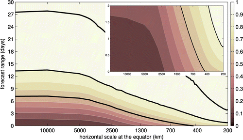
Figure 7. The growth of global forecast errors towards the saturation based on ECMWF data in May 2015. The errors F(t) are computed independently for each k and normalized by their values at day 60 in each . The isolines are every 0.1 and thick black isolines correspond to 0.6 (bottom), 0.9 (middle) and 0.99 (top) values. The small figure in the upper right corner is the growth over the first 2 days of the forecast.

Now we discuss the scale-dependent error growth over extended periods. The outputs in Figs. 6 and 7 are obtained by fitting (15(15) ) independently to data for every zonal wavenumber . It is clear that Fig. 6(a) is a reliable reproduction of Fig. 2(b) whereas Fig. 6(b) extends the solution to 30-day range. Notice that Fig. 2(b) uses log–log axes whereas Fig. 6(a) applies log-linear representation to show the growth from the start of the forecast. Figure 6(c) provides a focused view of scales under 700 km. It illustrates how initially very rapid growth (i.e. ) in small scales slows down. In 1.5. day forecast range the growth is smallest at the smallest scales and the growth rate increases going towards 700 km scale.

Figure 8. Parameters of the model (3(3) ) by Dalcher and Kalnay (1987) computed from Equations (23(23) ) to (24(24) ) based on ECMWF data in May 2015.

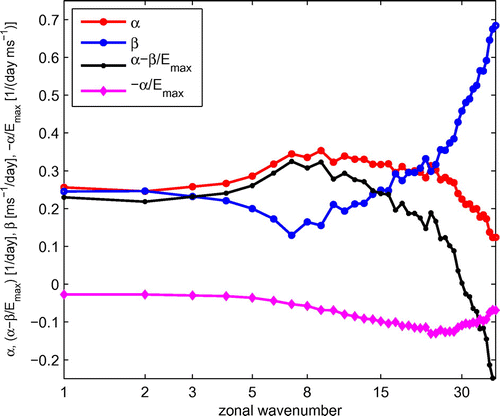
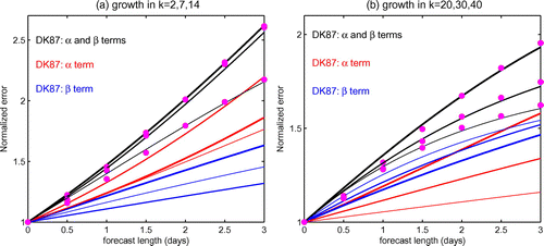
Figure 9. Comparison between the two terms of Dalcher and Kalnay (1987) model with ECMWF data for May 2015 in several zonal wavenumbers. (a) wavenumbers 2, 7 and 14, (b) wavenumbers 20, 30 and 40. Shown are solutions for the growth if only term is used (red curves), growth obtained with the term (blue curves) and the results for the sum of the two terms (black curves). Empirical data are added as circles. Solutions for various zonal wavenumbers are shown by curves of different thickness. The thickest line is for and , the medium thickness applies to and whereas the thin curves are solutions for and .

In Fig. 7, the errors are normalized by their asymptotic values at day 60 to present a scale-dependent perspective of atmospheric predictability in the state-of-the-art ENS. The three thick curves correspond to the 60, 90 and 99% of the saturation value in each scale. There is no standard definition of the percentage of saturation value to be used to define useful forecasts. In analogy to the anomaly correlation coefficient, which is used to evaluate the 500 hPa level in NWP models (Murphy and Epstein, 1989), we can use the 60% curve to discuss the useful global prediction skill as a function of scale. It suggests that at synoptic and larger scales, the useful prediction skill is around 1 week. This is similar to the estimate of the global average range of useful deterministic prediction based on 60% of the climatological variability in independent data (uncorrelated analyses) in Žagar et al. (2015a) and the criterion of 60% of the anomaly correlation coefficient for the 500 hPa geopotential height in the ECMWF deterministic system (e.g. Haiden et al., 2014). Based on the same 60% criterion, there is no useful prediction skill under 400 km scale in the applied data-set. On the other hand, if we use the 90% curve, it suggests that in our data there is some prediction skill in the smallest scales around 200 km the first day and in large scales up to about 2 weeks. There is a large gap between 90 and and 99% curves, a range with a slow exponential growth described by Equation (21(21) ). According to 99% saturation curve, an upper limit of the global prediction would be around 4 weeks for the planetary scales and around 2 weeks for smaller synoptic scales (several thousand km). The result for small scales can be considered most uncertain as the initial growth is largely defined by simulated analysis uncertainties that may not be optimal. However, it is not guaranteed that forecast errors determined by verifying forecast against an analysis (instead of using the ensemble spread as done here) would provide different results as the analysis at small scales is heavily influenced by the model background forecast.

4.2. Comparison with the model by Dalcher and Kalnay (1987)

Figure 8 shows the scale dependency of fitted parameters translated into and parameters of the standardly used model of Dalcher and Kalnay (1987), for data-set from May 2015. For the planetary scales, both values are between 0.2 and 0.3 per day. These values are similar to the estimates by Magnusson and Källén (2013) for the deterministic ECMWF model 500 hPa geopotential height and by Herrera et al. (2016) for 500 hPa height in several ensemble prediction systems. The similarity stems from the fact that variability at 500 hPa is dominated by large scales. As and have different units, their relative contributions to the error growth require comparison of the and terms of Equation (3(3) ). This is shown for several wavenumbers in Fig. 9 which is obtained by numerically solving (3(3) ) separately for the two terms for every wavenumber with input , and from the new model and .

We can notice in Fig. 9(a) that the two terms contribute similarly large parts of the error growth in the planetary scales during the first few days. We also notice that they are more similar for and than for . For this wavenumber, (Fig. 8) and the relative contribution of the term in comparison to the term increases with the forecast lead time (Fig. 9(a)). In 3-day forecast, the term is more than twice larger than the term for which can be compared to their 10% difference in (Fig. 9(a)). The growth curves for large wavenumbers have concave upward shape similar to that for 500 hPa geopotential field (e.g. Simmons and Hollingsworth, 2002).

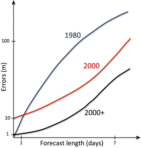
Figure 10. Sketch of the evolution of forecast errors of geopotential height at 500 hPa. Top line is based on the curves from Lorenz (1982) and errors estimated from forecast differences which show the error growth in the perfect model. The red curve shows the forecast errors based on Simmons and Hollingsworth (2002) with analysis errors estimated around 10 m in late 1990s. More recent curves found in various studies indicate S-shape in relation to a slow initial growth and a faster growth lateron.

As the wavenumber increases, grows and beyond wavenumber around 25 (Fig. 8). Correspondingly, Fig. 9(b) shows that for larger wavenumbers the term contributes a larger component of the error growth. Note also that the error curves in smaller scales are concave downward, i.e. opposite from the concavity in largest scales and that the downward concavity stems from the term. The fact that the term dominates at mesoscale is only seemingly in conflict with the previously shown exponential regime in these scales in Fig. 4. We must notice here that term of (3(3) ) mimics the Leith’s model (1(1) ) for the error growth if we replace and S in (1(1) ) by and , respectively. Thus, with only term retained, the solution of (3(3) ) is . With increasing at small scales whereas becomes smaller (Fig. 8), the exponential error growth at small scales is increasingly produced by the term. In relation to several previous studies, we notice that interpreting the term of (3(3) ) as the linear error growth associated with model deficiencies does not provide a full picture of the associated error dynamics.

5. Discussion and conclusions

In this paper we have assessed the scale-dependent growth of the global forecast uncertainties in the operational ECMWF ENS. Provided the ensemble of forecasts is reliably simulating the probability density function of future state of the atmosphere, the growth of the ensemble spread can be used as a proxy of the forecast error growth.

We have derived a new parametric model to represent the error growth. The new model is a more robust numerical alternative to the commonly used model of Dalcher and Kalnay (1987) for fitting the empirical data. The chaotic nature of atmospheric system is evidenced in the exponential growth of errors (). According to the parametric model of Dalcher and Kalnay (1987), the error growth curves are concave downward as seen in large-scale forecast errors computed from forecast differences in 1980s (e.g. Lorenz, 1982). This is illustrated in Fig. 10. As the initial state for NWP improved and models’ resolution increased, the error growth curves changed in 1990s to being concave upward (e.g. Simmons and Hollingsworth, 2002). Depending on the selected variable and region, the average statistics of error growth can be more complex with concavity changing sign, particularly at large scales. A combination of hyperbolic tangent functions in our parametrization of the growth proves robust to reliably model such complex dynamics of the growth across many scales. In contrast to the models (1(1) )–(3(3) ), the new model does not involve computation of the time derivatives. The asymptotic error is not a fitting parameter, but it is computed from the model constants.

The new fitting function has been applied independently to every scale of the simulated ECMWF errors. According to the new fit, the range of useful prediction skill, estimated as a scale when the growth of simulated forecast errors reaches 60% of their asymptotic values is around one week in large scales and 2–3 days at 1000 km scale. These estimates appear realistic in comparison with the anomaly correlation criteria used in the global NWP models, primarily on large scale. It takes 10 days to 2 weeks for the synoptic and planetary-scale errors, respectively, and only about a day for errors at 200-km scale to reach 90% of their values at day 60. This quantifies a scale-dependent increase of the period of a slow exponential growth which is described by a special analytical solution of the new model.

The parameters and of the model by Dalcher and Kalnay (1987) can easily be computed from parameters of the new model. The comparison of the two parameters shows that their values diverge beyond the zonal wavenumber 15 (around 1000km scale in the extra-tropics). At small scales, the term describes most of a rapid exponential growth of errors towards saturation.

Acknowledgements

We would like to thank anonymous reviewers for their comments and to Prof. Eugenia Kalnay and Prof. Dale Durran for their comments on an earlier version of this manuscript. Dr. Nils Gustafsson and Prof. Peter Lundberg are thanked for their advice and for handling the paper.

Additional information

Funding

Research of Nedjeljka Žagar is funded by the European Research Council (ERC), Grant Agreement Number [280153], MODES. The input data for this study were provided by the ECMWF, http://www.ecmwf.int.

Notes

No potential conflict of interest was reported by the authors.

Appendix 1

Connection between the error growth model and the logistic function

The logistic function is a reciprocal exponential function shifted in value and argument and typically written as(A1)

where is its midpoint, k is the steepness of the curve, L is the scaling factor and K is the shift in value. By expressing hyperbolic tangents using exponential functions

we can rewrite the model function for E(t) (9(9) ) into logistic function (A1(A1) ) and thereby revealing relationships between the coefficients of the two functions:

Notice that parameters k and K in the last expression have no relations to those used earlier in the paper.

References

- Bengtsson, L. K., Magnusson, L. and Källén, E. 2008. Independent estimations of the asymptotic variability in an ensemble forecast system. Mon. Weather Rev. 136, 4105–4112.
- Buizza, R., Leutbecher, M. and Isaksen, L. 2008. Potential use of an ensemble of analyses in the ECMWF Ensemble Prediction System. Q. J. Roy. Meteor. Soc. 134, 2051–2066.
- Buizza, R., Miller, M. and Palmer, T. N. 1999. Stochastic representation of model uncertainties in the ECMWF EPS. Q. J. Roy. Meteor. Soc. 125, 2887–2908.
- Buizza, R. and Leutbecher, M. 2015. The forecast skill horizon. Q. J. Roy. Meteor. Soc. 141, 3366–3382.
- Dalcher, A. and Kalnay, E. 1987. Error growth and predictability in operational ECMWF forecasts. Tellus 39A, 474–491.
- Düben, P. D., Joven, J., Lingamneni, A., McNamara, H., De Micheli, G., and co-authors. 2014. On the use of inexact, pruned hardware in atmospheric modelling. Philos. Trans. Roy. Soc. London A. 372(2018), 20130276. doi: 10.1098/rsta.2013.0276. Online at: https://www.ncbi.nlm.nih.gov/pubmed/24842031
- Haiden, T. and co-authors. 2014. Evaluation of ECMWF forecasts, including 2013--2014 upgrades. ECMWF Tech. Memorandum. 742. Online at: http://www.ecmwf.int
- Harlem, J., Oczkowski, M., Yorke, J. A., Kalnay, E. and Hunt, B. R. 2005. Convex error growth patterns in a global weather model. Phys. Rev. Lett. 94, 228501. Online at: https://www.ncbi.nlm.nih.gov/pubmed/16090440
- Herrera, M., Szunyogh, I. and Tribbia, J. 2016. Forecast uncertainty dynamics in the THORPEX Interactive Grand Global Ensemble (TIGGE). Mon. Weather Rev. 144, 2739–2766.
- Isaksen, L., Bonavita, M., Buizza, R., Fisher, M., Haseler, J. and co-authors. 2010. Ensemble of data assimilations at ECMWF. ECMWF Tech. Memorandum 636. Online at: http://www.ecmwf.int
- Jung, T. and Leutbecher, M. 2008. Scale-dependent verification of ensemble forecasts. Q. J. Roy. Meteor. Soc. 134, 973–984.
- Kasahara, A. 1976. Normal modes of ultralong waves in the atmosphere. Mon. Weather Rev. 104, 669–690.
- Kuhl, D., Szunyogh, I., Kostelich, E. J., Patil, D. J., Gyarmati, G. and co-authors. 2007. Assessing predictability with a local ensemble Kalman filter. J. Atmos. Sci. 64, 1116–1140.
- Leith, C. E. 1978. Objective methods for weather prediction. Annu. Rev. Fluid Mech. 10, 107–128.
- Lorenz, E. 1982. Atmospheric predictability experiments with a large numerical model. Tellus 34, 505–513.
- Lorenz, E. 1996. Predictability -- a problem partly solved. In: Predictability of Weather and Climate (eds. T. Palmer and R. Hagedorn). Cambridge: Cambridge University Press, pp. 40–58.
- Magnusson, L. and Källén, E. 2013. Factors influencing skill improvements in the ECMWF forecasting system. Mon. Weather Rev. 141, 3142–3153.
- Murphy, A. H. and Epstein, E. S. 1989. Skill scores and correlation coefficients in model verification. Mon. Weather Rev. 117, 572–582.
- Palmer, T. N. and co-authors. 2009. Stochastic parametrization and model uncertainty. ECMWF Tech. Memo. 598. Online at: http://www.ecmwf.int
- Park, Y.-Y., Buizza, R. and Leutbecher, M. 2008. TIGGE: Preliminary results on comparing and combining ensembles. Q. J. Roy. Meteor. Soc. 134, 2029–2050.
- Rotunno, R. and Snyder, C. 2008. A generalization of Lorenz’s model for the predictability of flows with many scales of motion. J. Atmos. Sci. 65, 1063–1076.
- Reynolds, C. A., Webster, P. J. and Kalnay, E. 1994. Random error growth in NMC’s global forecasts. Mon. Weather Rev. 122, 1281–1305.
- Savijärvi, H. 1995. Error growth in a large numerical forecast system. Mon. Weather Rev. 123, 212–221.
- Shutts, G. J. 2005. A kinetic energy backscatter algorithm for use in ensemble prediction systems. Q. J. Roy. Meteorol. Soc. 131, 3079–3100.
- Simmons, A. J., Moreau, R. and Petroliagis, T. 1995. Error growth and predictability estimates for the ECMWF forecasting system. Q. J. Roy. Meteorol. Soc. 121, 1739–1771.
- Simmons, A. J. and Hollingsworth, A. 2002. Some aspects of the improvement in skill of numerical weather prediction. Q. J. Roy. Meteor. Soc. 128, 647–677.
- Simmons, A. 2006. Observations, assimilation and the improvement of global weather prediction -- some results from operational forecasting and ERA-40. In: Predictability of Weather and Climate (eds. T. Palmer and R. Hagedorn). Cambridge: Cambridge University Press, pp. 428–458.
- Žagar, N., Buizza, R. and Tribbia, J. 2015a. A three-dimensional multivariate modal analysis of atmospheric predictability with application to the ECMWF ensemble. J. Atmos. Sci. 72, 4423–4444.
- Žagar, N., Kasahara, A., Terasaki, K., Tribbia, J. and Tanaka, H. 2015b. Normal-mode function representation of global 3D datasets: An open-access software for atmospheric research community. Geosci. Model Dev. 8, 1169–1195.