Comparing the linear and nonlinear buoyancy-driven circulation

Abstract

The buoyancy-driven circulation is studied in an idealized domain using two models, one based on the linearized planetary geostrophic equations and a fully nonlinear GCM. The surface buoyancy is specified (relaxed) to a chosen function of latitude in the linear (nonlinear) model. The models yield similar baroclinic flow in the interior, where the surface velocities are primarily zonal, and near the southern boundary, where a westward surface flow feeds the western boundary current (WBC). They differ however in the north. While the linear model has westward surface flow of limited vertical extent near the northern wall, the GCM has baroclinic flow which extends to the bottom with eastward surface velocities. The difference is due to convection, which weakens the stratification in the nonlinear model, amplifying the thermal wind transport associated with the surface buoyancy gradient. The WBC flow in the GCM feeds this, with northward surface flow over its entire length (as seen in nearly all previous similar studies). This in turn determines the meridional overturning circulation, since the WBC accounts for the largest meridional velocities. Roughly half the upwelling occurs in the WBC in the GCM and half in the interior, while the upwelling occurs in the interior and near the southern wall in the linear model. The study highlights the role of convection in modifying the response to the surface buoyancy gradient.

Keywords:

• meridional overturning circulation
• boundary currents
• thermocline
• buoyancy-driven flow

1. Introduction

The oceanic meridional overturning circulation (MOC) plays a central role in the global redistribution of heat and trace gases in the climate system (Ganachaud and Wunsch, 2000; Lumpkin and Speer, 2007). With time scales of hundreds to thousands of years, it contributes to long term climatic variability, and as such the MOC has become a major research area. But which mechanisms drive the MOC is still debated (e.g. Kuhlbrodt et al., 2007). The MOC is usually studied with fully coupled general circulation models (GCMs), with an ocean forced by winds and surface heat and freshwater fluxes. Such studies reveal many interesting aspects. But the complexity of GCMs can obscure the relative importance of different forcings.

Both the wind- and buoyancy-driven circulations exhibit intensified western boundary currents (WBCs). So the northward flow towards the convection sites in the North Atlantic is superimposed on the Gulf Stream which closes the wind-driven subtropical gyre. Indeed the buoyancy-driven circulation is often conflated with the Gulf Stream, causing confusion in the media (e.g. Wunsch, 2004). Furthermore, wind and buoyancy forcing can act in tandem; indeed the buoyancy-driven circulation would not exist without vertical mixing (Sandström, 1908; Paparella and Young, 2002), a large fraction of which is due to the winds. But this complicates assessing how the MOC would change if one or another forcing were altered.

The buoyancy-driven circulation has been studied in the absence of explicit wind forcing though, to understand the response to surface buoyancy fluxes alone. Many such studies have been made in idealized geometries, like a rectangular box (Bryan, 1987; de Verdiere, 1988; Marotzke97; Huck et al., 1999; Marotzke and Scott, 1999; Park and Bryan, 2000; Park and Bryan, 2001; Huck and Vallis, 2001; Park, 2006). The surface flux is imposed, as is the vertical mixing. The result is usually an MOC comparable in strength to that observed in full GCMs, despite the lack of wind forcing. Such simulations have been used to study the dependence on convective mixing (Marotzke and Scott, 1999), the choice of vertical coordinate (Park and Bryan, 2000; Park and Bryan, 2001) and horizontal resolution (Park, 2006).

These simulations exhibit similar features. The surface flow in the interior (away from the lateral boundaries) is generally zonal and in thermal wind balance with the surface density gradient. Sinking occurs in the northern part of the domain, producing a prominent deep WBC. The sinking occurs primarily in frictional boundary layers near the basin walls and as such, the overturning depends on the choice of frictional schemes (Huck et al., 1999).

Idealized domains also permit analytical solutions. Assuming the background stratification is fixed and neglecting the advection of buoyancy and momentum, one can obtain a full solution to the steady circulation. The linear model (Pedlosky, 1969; Salmon, 1986) yields a circulation broadly like that in the nonlinear numerical solutions, with zonal interior flow and vertical motion confined to boundary layers near the walls. The model has been used to study the dependence on mixing (LaCasce, 2004), vertical velocities (Pedlosky and Spall, 2005) and the role of eastern boundary currents (Cessi and Wolfe, 2009; Cessi et al., 2010).

Other theoretical models have also been employed to study aspects of the buoyancy-driven circulation. In a seminal study, Stommel and Arons (1960) examined the circulation in an abyssal layer due to localized downwelling and uniform upwelling. Kawase (1987) modified their model by adding parameterized upwelling in the interior. Pedlosky and Spall (2005) examined a two layer model, as a simplified representation of the linear model, and considered (among other things) the effect of transport to other basins. Schloesser et al. (2012) proposed a multi-layer model, in which temperature could vary laterally in the upper layer. These models display many similarities to the numerical solutions noted above. But being layer models, employing parameterizations for vertical mass exchange and assumptions about the vertical density structure, they do not lend themselves as readily as the linear model to a direct comparison with a GCM, under identical forcing and basin configurations.

Such a comparison is the present goal. The exercise sheds light on both applicability of the linear model and on aspects of the circulation in the nonlinear models. While the linear model captures several important aspects, particularly at lower latitudes, it fails at higher latitudes where convection is acting. Describing how convection modifies the nonlinear solution is the second goal of the paper.

The linear model is outlined in Section 2 (further details are given in Appendix 1) as is the numerical model used here. The results are compared in Section 3 and the conclusions presented thereafter.

2. Model description: linear model

The linear model employs the steady planetary geostrophic (PG) equations (e.g. Samelson, 2011). Without wind forcing, these are:(1) (2) (3) (4) (5) Here b is the buoyancy, is the lateral viscosity and and are horizontal and vertical diffusivities. The first four equations are common with the nonlinear PG equations (e.g. de Verdiere, 1988), but the buoyancy equation is modified by omitting time dependence and horizontal advection. And vertical advection is linearized about a prescribed background stratification, , which is assumed constant.

The lateral friction terms in the geostrophic relations permit no normal flow and no slip at the lateral walls.¹ Lateral mixing in the buoyancy equation is meant to mimic eddy mixing. Under the assumption of a constant background stratification, this is equivalent to the Gent and McWilliams (1990) parameterization (Cessi and Wolfe, 2009).

The rectangular domain spans the range , , . We assume no buoyancy fluxes normal to the lateral walls and bottom, and we specify the buoyancy at surface²:(6)

We assume the surface buoyancy is a linear function of y, i.e. , if is the value at mid-basin.

The advantage of the PG equations is that they can be reduced to a single equation with one dependent variable (Welander, 1971). With the linear buoyancy equation, an equation for pressure is obtained:(7)

The term on the LHS comes from the advection of planetary vorticity, while the terms on the RHS are vertical mixing, horizontal mixing and horizontal friction, respectively. Scaling the terms in (7(7) ) and dividing by the scale of the first term, , yields:

For reasonable values of and , the last two terms are small except near the boundaries. So the balance in the interior is between the first two terms, which yields the thermocline depth:(8)

where L is the basin scale. With the parameters used hereafter, this is roughly 400 m. The dependence of contrasts with that obtained for the nonlinear equations, of (Bryan, 1987; de Verdiere, 1988; Vallis, 2006). The difference stems from specifying in the linear solution. Note the depth is only weakly sensitive to in the linear solution; decreasing by a factor of 10 reduces the thermocline depth by only a factor of 1.8.

The zonal velocity exhibits a similar vertical scaling because:

from thermal wind. With typical parameters, u is of order 1 cms

In the interior, the horizontal velocities are geostrophic and the Sverdrup relation holds:(9)

Thus with a flat bottom and a rigid lid there is no depth-integrated flow.

The equation governing the interior flow (involving the first two terms in Equation 7(7) ) is easily solved following a Fourier cosine transform:(10)

The resulting ODE in x is solved by integrating westward from the eastern boundary (at ), yielding:(11)

where:

and where is the pressure on the eastern wall. Thus the interior meridional velocity:(12)

decays exponentially from the eastern wall. The higher baroclinic modes decay much more rapidly than the lower ones, implying the flow deepens to the west. The vertical velocity, obtained from the Sverdrup relation, is similarly intensified in the east.

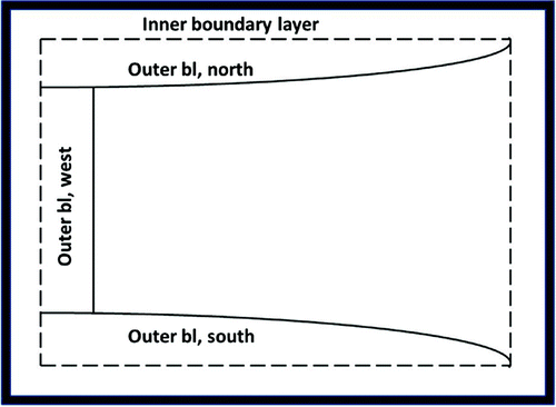
Figure 1. The boundary layer structure in the linear model.

The pressure, , is constant to prevent normal flow at the eastern boundary. It is determined by demanding that the basin-integrated vertical velocity vanish (details are given in Appendix 1). The interior flow is dominated by the zonal component, in thermal wind balance with the buoyancy gradient at the surface.

The boundary layer structure is sketched in Fig. 1. No normal flow is satisfied on the three non-eastern walls in the outer of two frictional boundary layers. On the north and south walls, the balance in the outer layer is between the first three terms in Equation (7(7) ). The meridional width can be shown to scale as:(13)

where D is the thermocline depth above. is of order 1000 km, with the present parameters. On the western wall, it is the first and third terms which balance in the outer layer, referred to as a “thermal” layer (Pedlosky and Spall, 2005). The layer width scales as:(14)

This is of order 200 km with the present parameters.

In addition, there is a thin inner layer on each wall (Fig. 1) which satisfies the no-slip condition, the “hydrostatic” layer (Pedlosky and Spall, 2005; Schloesser et al., 2005). In this, the third and fourth terms in Equation (7(7) ) balance, i.e. the lateral buoyancy mixing and horizontal friction terms. The layer is very narrow, with a width which scales as:(15)

where is the Prandtl number. Assuming Pr is order one, the width is comparable to the deformation radius based on the thermocline depth, yielding km. The hydrostatic layers have large vertical velocities. However the net vertical transport in the layer is balanced by opposing transport in the outer layer (Appendix 1). Thus in each double boundary layer there is no areally-integrated vertical transport from horizontal mixing (although there is a net contribution from vertical mixing, as seen below).

If is large enough, the double western boundary layer is replaced by a single Munk layer (Pedlosky, 1969; LaCasce, 2004). However it can be shown that the areally-integrated vertical velocity vanishes in this case as well. Thus having a western Munk layer has relatively little effect on the interior circulation in the linear model.

3. Model description: MITgcm

For the numerical simulations, we use the Massachusetts Institute of Technology general circulation model (MITgcm) (Marshall et al., 1997a, b). The model was run in an ocean-only configuration, with no sea ice or wind forcing. We employed a horizontal resolution of and 24 vertical levels spanning 6 km, with 20 m vertical resolution in the upper layers increasing to 900 m at depth.

A linear equation of state was used and the salinity was kept constant, so that changes in buoyancy were due solely to temperature. The surface temperature was relaxed to a profile of , with a relaxation time of one month. The latter can impact the stability of the solutions (e.g. Power and Kleeman, 1993), but we kept this fixed for present experiments. The model was spun up from a homogeneous rest state with a temperature of C and it was run for 5500 years, by which time the solution was in a steady state.

For the mixing coefficients we used ms and ms. Both vary in space in reality, being intensified near ocean boundaries (e.g. Ledwell and Bratkovich, 1995a, b), but we kept both constant for comparison with the analytical solution. Convection is represented through enhanced vertical mixing (Klinger et al., 1996), in that is set to 100 ms under unstable conditions. Lastly, a fairly large horizontal viscosity ( ms) was required, to maintain stability.

Figure 2. Horizontal velocity at the surface in the linear model (left) and MITgcm (right). The arrows indicate the direction and the colors indicate the strength of the flow.

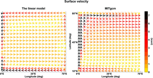
Figure 3. Mid-basin transects of the zonal velocity at E in the linear model (left) and in MITgcm (right).

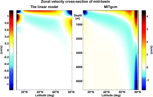
Figure 4. Cross-sections of the meridional velocity at N (lower row) and N (upper row) for the linear model (left column) and MITgcm (right column).

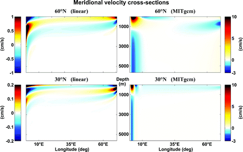
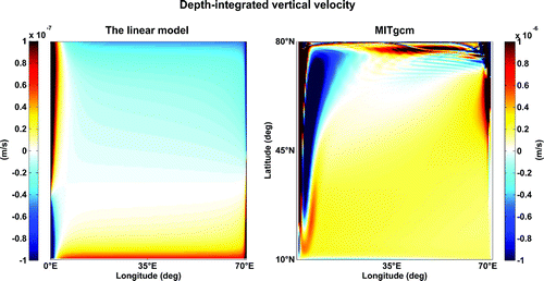
Figure 5. Depth-integrated vertical velocity for the linear model (left) and MITgcm (right). In the north and south, only the vertical velocities associated with vertical mixing are shown, as only these contribute to the area-averaged w. The wave-like disturbances in the north in the MITgcm simulation are linked to convection (rather than numerical instability).

4. Results

4.1. Comparing the models

The surface velocities from the two models are shown in Fig. 2. The interior velocities in the linear model (left panel) are primarily zonal, in thermal wind balance with the surface temperature gradient. The flow diverges at the eastern boundary, turning south in the southern part of the domain and north in the northern. The latter is the model’s North Atlantic Current, bounding the warmer waters adjacent to the eastern boundary and the colder interior waters (e.g. Mauritzen, 1996). In both the north and south the flow turns westward along the respective boundaries and then towards the mid-basin along the western boundary. The WBCs, the strongest flows in the domain, feed the interior and close the circulation.

The interior flow in the GCM (right panel) is also zonal at the surface and veers north and south at the eastern boundary. As noted by Park (2006), this turning is missed in models with coarser resolution (and is difficult to see in this figure as well). As in the linear model, the flow in the southeast turns west at the southern boundary, feeding a boundary current which proceeds to the western boundary. But the flow near the northern boundary is eastward. As such the flow in the WBC, which feeds the northern flow, is northward over the full range of latitudes. Such surface flow is typical in simulations like this (e.g. de Verdiere, 1988; Marotzke, 1997; Huck et al., 1999; Park and Bryan, 2000).

The difference in the zonal flow is highlighted in a mid-basin transect, along E (Fig. 3). In the linear model, the flow is confined to the upper 2000 m. The velocities are eastward in the interior over the upper several hundred meters. The depth of the eastward flow increases to the north, consistent with the dependence indicated by the scaling in Equation (8(8) ). The flow below that is westward, and this contributes to making the depth-averaged velocity zero. Boundary currents with opposed baroclinic flow are seen at the north and south walls, and these also have zero depth-averaged transport. The depth of the flow is shallower at the southern boundary as f is smaller than at the the northern boundary. Note how the westward interior flow shallows to join the westward surface flow at the southern wall.

The GCM also exhibits eastward flow at the surface, westward flow below and a zero crossing depth which increases with latitude. The westward interior flow joins the surface return flow at the southern boundary as in the linear model. The solution differs though at the northern wall, where there is eastward flow to 2000 m and westward flow below that to the bottom. The velocities moreover are roughly 5 times larger than in linear model.

Fig. 4 shows cross sections of the meridional velocity in the two models, at N and N. In the linear model (left panels) the flow is mostly confined to the upper 2500 m. The flow depth increases from east to west, reflecting the more rapid decay of the higher baroclinic modes from the eastern boundary (Section 2). The surface flow at the eastern boundary is northward at N and southward at N, and there are opposing flows at depth. The flows on the eastern wall are linked to similarly oriented, but deeper, flows on the western boundary. The surface flow at the western boundary is toward the mid-basin at both latitudes.

In the GCM there is also baroclinic flow along the eastern boundary (right panels of Fig. 4), with northward surface flow at N and southward flow just below the surface at N. But the flow in the western boundary layer is entirely different, with a vertical structure resembling the first baroclinic mode and spanning the entire depth. The flow is northward at the surface and southward below 1000 m (the latter being the model’s Deep Western Boundary Current) and the structure is the same at both latitudes. The WBC is clearly feeding the flow near the northern wall (Fig. 3), which has the same vertical structure. Opposed baroclinic flow is seen offshore at both latitudes, suggestive of a recirculation.

The differences are more striking with the vertical velocities (Fig. 5). These vary significantly with depth, but we show the depth-integrated field for simplicity. In the linear model there is sinking in the north, where the imposed surface temperature anomaly is negative, and upwelling in the south, where it is positive. The transport in the northern, southern and eastern boundaries is consistent with that in the adjacent interior regions, but it is also stronger (we contour only the portions which contribute to the net up/downwelling). In the western layer there is intense upwelling in the north and sinking in the south.

As noted, the transport in the inner boundary layer in the west opposes that in the outer layer, and the area-integrated contributions cancel. Thus the strong upwelling in the northern part of the western boundary layer is canceled by downwelling next to the wall, in the no-slip layer (not visible in this figure). The net contributions to the vertical transport occur in the interior, in the outer layers (due to vertical mixing) in the north and south and in the single no-slip layer in the east. With the parameters used here, the interior and N/S boundary layer contributions are largest.

The sign of w in the boundary layers can be understood as follows. In the west, lateral mixing dominates the right hand side of the buoyancy equation in Equation (5(5) ):(16)

after invoking the hydrostatic relation. Furthermore the meridional velocity is geostrophic, so:(17)

In the northern part of the outer western boundary layer, is negative (the surface flow is southward) so and w are positive. But is negative in the inner layer, due to the no-slip condition, so w is negative there. In the southern part of the western boundary layer the results are reversed because the surface flow is northward.

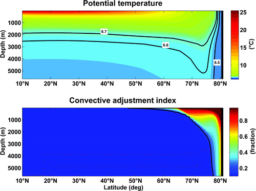
Figure 6. Zonally averaged potential temperature (top) and convective adjustment index (bottom). In areas where the index is greater than zero, the vertical diffusivity is large due to enhanced mixing.

The GCM also exhibits strong upwelling in the western boundary layer (right panel). However, there is no opposed downwelling near the wall. Rather, there is a large region of downwelling offshore, in the recirculation seen in Fig. 4. Integrating across the two layers one finds that the downwelling only partially compensates the near-boundary upwelling, so the western boundary layer is a net upwelling site in the model. The balances in the WBC are examined further in Section (4.3).

The interior is also an upwelling region in the GCM (Fig. 5). Where then is the flow downwelling? The wavy region in the north indicates where convection is occurring, but w is both positive and negative here. The major downwelling site rather is in the northeast corner, where the eastward flowing current (Fig. 2) impacts the eastern boundary (e.g. de Verdiere, 1988; Marotzke and Scott, 1999). As such the w field resembles that imagined by Stommel and Arons (1960), with a localized source in the north and quasi-uniform interior upwelling. However significant upwelling also occurs in the western boundary layer, as seen by Kawase (1987).

There are also large vertical velocities in the no-slip layers along the southern, eastern and northern walls. The sign of w is consistent with that in the linear model boundary layers, where the tangential velocity is in thermal wind balance and w is balanced by lateral mixing. So near the northern wall, for example: is positive and negative near the wall, so w is positive.

The other major difference between the models is the zonally-averaged stratification, shown for the GCM in the upper panel of Fig. 6. The thermocline in the south is confined to the upper 1000 m, but the isotherms outcrop at the northern latitudes. The profile is typical for such simulations (including those with wind-forcing) and in the ocean as well (e.g. Talley et al., 2003; Marshall and Plumb, 2007). But it differs markedly from the linear model, which assumes a constant stratification over the full range of latitudes.

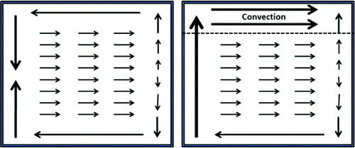
Figure 7. A schematic illustrating the differences in the surface flow between the linear and nonlinear models.

The northern stratification is weakened by convection (lower panel). The zonally-averaged convective index shows that convection occurs at shallower levels to N, but extends to the bottom north of N. The region where u differs so profoundly from the linear model, in Fig. 3, is precisely where convection reaches the bottom.

The similarities and differences between the two models are summarized in the schematic in Fig. 7. Both have eastward surface flow in the interior that veers north or south at the eastern wall. But convection in the GCM (right) reduces the stratification in the north. The surface flow is also eastward in this region, the surface expression of a baroclinic flow which extends to the bottom. The horizontal flow in the convective region is linked to a WBC with the same vertical structure. The linear model (left), with constant stratification, has instead a two-gyre circulation and its boundary layers feed the interior flow.

4.2. Convection in the GCM

Thus the major differences between the models are due to convection in the nonlinear model. As noted, convection in the MITgcm is parameterized as intensified vertical diffusion. This rapidly mixes buoyancy in the vertical, driving the temperature towards a linear vertical gradient and hence a constant (and small) N.

Thus the buoyancy equation in the convective region is dominated by vertical mixing, i.e. . This implies that the third derivative of the pressure vanishes, from the hydrostatic relation. So the pressure in the convective region has the form:

The coefficient, B, is determined by the imposed buoyancy gradient at the surface:

assuming the relaxation time for the surface temperature is sufficiently short. The constant A is found by imposing zero buoyancy anomaly on the lower surface:

Then C is determined from the requirement of no depth-averaged flow. The final result is:(18)

The horizontal velocities have the same vertical structure, from geostrophy.

The velocity profile, averaged over the region where convection reaches the bottom, is compared to that predicted in Equation (18(18) ) in the left panel of Fig. 8. While not exact, the similarity is strong enough to support the preceding arguments. The mean stratification in the region is much weaker than in the region south of the convective zone (right panel of Fig. 8). In fact it exhibits some vertical variation, but it is more nearly constant in specific locations. The velocity profile resembles the first baroclinic mode, with a single zero crossing near 2500 m. However the shear is non-vanishing at the surface, to match the surface temperature gradient. Thus it is the temperature gradient at the surface which is ultimately responsible for horizontal transport in the convective region.

Figure 8. Left: A vertical profile of the mean zonal velocity in the convective region in MITgcm (blue line) and calculated according to Equation (18(18) ) (yellow line). Right: The mean stratification in convective region (blue line) and just south of the convective region (yellow line) in MITgcm.

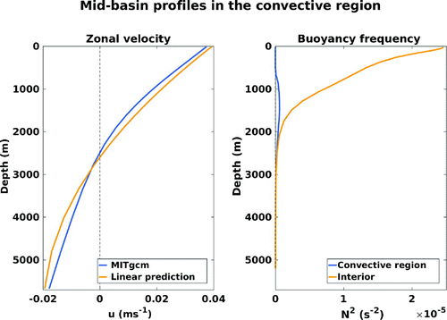
Figure 9. Horizontal (blue arrows and numbers) and vertical (boxes - red numbers indicate upwelling while blue numbers indicate downwelling) transports for the upper 1200 m in MITgcm. All transports are given in Sv.

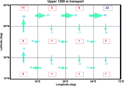
The net effect is illustrated in Fig. 9, which shows horizontal and vertical transports in chosen regions in the upper 1200 m. The near-surface flow is not confined to this range of depths, but using a constant depth is simpler and permits the transports to balance in each region (the transports below 1200 m are generally the opposite of these). Consider the NE box. There is 38 Sv entering from the west; this is the portion of the eastward flowing current in Fig. 3 above 1200 m. Most of this sinks (33 Sv), making this the major downwelling site in the model. A smaller portion (5 Sv) flows south, along the eastern boundary. The surface flow along the northern portion of the eastern boundary is northwards (Fig. 4), but there is southward flow beneath and this dominates the total transport over the upper 1200 m.

Figure 10. The meridional overturning streamfunction, , for the (top) linear model and (bottom) MITgcm. Positive indicates clockwise rotation. Top figure: The linear model exhibits two overturning cells confined to the southern and northern part of the basin. Bottom figure: MITgcm exhibits one positive overturning cell spanning the basin and one narrow, negative cell in the north. The latter is a consequence of the no-slip condition at the northern wall.

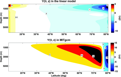
Figure 11. Maximum overturning (dark blue), northern boundary layer width (light blue), north-east downwelling (red), meridional heat transport at N (brown) and heat transport in the southern boundary layer (green) sensitivity to vertical mixing, . The maximum overturning include three values from Winton (1996), scaled by 0.7.

The box to the west of that in the NE corner has 33 Sv entering from the west. It also has 6 Sv upwelling from below. This occurs in the no-slip boundary layer adjacent to the wall. These combine to feed the 38 Sv into the NE box (minus a small 1 Sv flow to the south). In the NW box, there is 20 Sv entering from the south, across N. There is also 11 Sv of upwelling, which occurs primarily in the WBC. Together these feed the 31 Sv flowing to the east. Without the upwelling from the no-slip layer on the northern wall, this 31 Sv would presumably proceed to the eastern wall and sink.

The meridional transport occurs primarily in the WBC. 9 Sv enters from the east, south of N, and this comes primarily from along the southern boundary. This is augmented by upwelling along the current, and by a further 5 SV from the east in the mid-latitudes. 6 of the 20 Sv crossing N upwells in the WBC, while another 7 Sv upwells in the interior. The remainder comes from horizontal circulation in the upper 1200 m.

The zonally-averaged overturning streamfunction, the MOC (lower panel of Fig. 10), is largely determined by the flow in the WBC. The amplitude of the primary cell is roughly 20 Sv, i.e. the same as that crossing N in the west in Fig. 9. The MOC derives from the vertical integral of the zonally-averaged meridional velocity, and the latter is by far largest near the western boundary. Calculating the MOC by integrating over only the western layer yields nearly the same result (not shown).

The overturning in the linear model (upper panel) is very different, with a weaker anticyclonic cell confined to the south. This is because the northward flow in the WBC occurs only in the south (Fig. 2). The cell is also shallower in the linear model, as the sinking is mostly confined to the upper thousand meters.

There is also the blue cell in lower panel of Fig. 10, which has the opposite sign (cyclonic) circulation. This is the flow associated with upwelling in the no-slip layer at the northern wall. Similar cells have been seen previously (e.g. Marotzke, 1997; Zhang et al., 1992). The cyclonic cell in the linear linear model comes instead from the southward surface flow in the model’s WBC.

But what sets the transport in the GCM? As noted, the flow in the convective region extends to the bottom, so integrating the eastward flow yields a transport which depends on the depth, H, but not on the vertical diffusivity. This is curious, because the MOC is known to vary with (e.g. Park and Bryan, 2000).

The reason is that the width of the convective region depends on . The northward surface flow along the western boundary brings warmer water into the convective region and this cools and convects. Increasing the northward transport causes the convective region to widen. The flow is in equilibrium when the heat lost at the surface is equal to the net meridional heat flux entering the northern region, which occurs primarily in the near-surface WBC.³

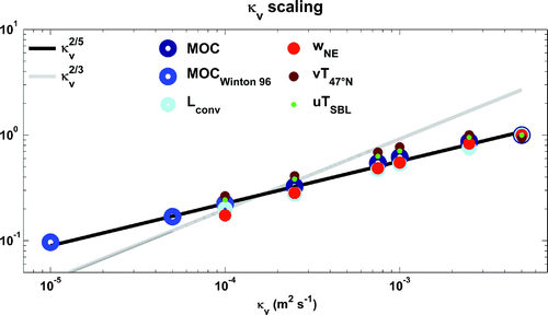
To test this, we conducted additional experiments with different values of , in the range from ms to  ms. The results (Fig. 11) indicate that the strength of the MOC co-varies with 1) the strength of sinking in the northeast, 2) the width of the convective region and 3) the meridional heat transport from the south. The different measures scale approximately as , somewhat slower than predicted from traditional scaling arguments (Welander, 1971) but in the range obtained in similar numerical simulations (Park and Bryan (2000) and references therein). Values from Winton (1996) are plotted for comparison.

Roughly three quarters of the transport in the WBC enters from the interior, and this flow scales as the other measures do. Having a larger vertical diffusivity yields more upwelling in the interior and a stronger current along the southern boundary. So the circulation in the thermocline region feeds that in the convective region, providing warm waters which sink. This also explains why the MOC, which reflects the flow in a region where vertical mixing is much larger than in the southern interior, nevertheless scales with .

For comparison, the width of the northern boundary layer in the linear model scales as (Section 2). So the layer actually contracts with increasing . But the comparison is misleading because the convective region in the GCM is not a traditional lateral boundary layer.

4.3. The western boundary current

The WBC is of primary importance to the MOC, accounting for most of the meridional flow from which the MOC derives. The greatest upwelling also occurs here. This implies that a significant portion of the MOC is essentially 2D.

In the linear model, the buoyancy equation is dominated by vertical advection and lateral mixing. In the GCM, the balance is more complex (Fig. 12), but is, approximately:

The same balance was seen by de Verdiere (1988). The vertical advection term is positive near the wall, where there is upwelling, and negative offshore in the recirculation region. This is balanced in part by meridional advection, which is negative over the region (because v is positive and is negative). Lateral mixing on the other hand is negative near the wall and positive offshore.

Figure 12. Terms in the buoyancy equation in the western boundary region, at N and 300 m depth from MITgcm.

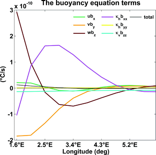
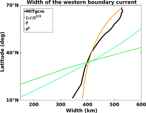
Figure 13. Scaling of the width of the western boundary current (black line) vs. Munk layer (orange line), the Coriolis frequency f (blue line) and (dark green line).

The sign of the lateral mixing follows from thermal wind, as discussed before, because the tangential flow is in geostrophic balance: is positive near the wall and negative in the recirculation region (note that the term shown in the figure has the opposite sign, indicating the effect on the LHS of the buoyancy equation).

Upwelling in the WBC is frequently seen in simulations like this and is usually attributed to the Veronis effect (e.g. Schloesser et al., 2012), spurious diapycnal mixing induced by horizontal mixing when the isopycnals aren’t horizontal (Veronis, 1975). However lateral mixing also dominates in the linear model, in which the Veronis effect is identically zero (because the base stratification is only a function of z). de Verdiere (1988) likewise argued that western upwelling is genuine and that lateral diffusion is a necessary ingredient in the adjustment to the boundary conditions.

In the linear model, the outer western boundary layer has a width which scales as (Equation 14(14) ). But the boundary layer width in the GCM scales instead as (Fig. 13), indicating a Munk layer. As noted, a fairly large horizontal viscosity, , is used in the simulation, to ensure numerical stability. Still, scaling the linear model with the same parameters suggests a double boundary layer structure. However, the linear model scaling assumes the WBC has a depth comparable to the thermocline depth, D. In the GCM, the WBC spans the entire water column. Using the total depth, H, instead of D, one can show that a Munk layer scaling is appropriate in the WBC. So convection also indirectly alters the dynamical balance in the WBC.

The linear model can be solved with a western Munk layer (Pedlosky, 1969; LaCasce, 2004). Though the detailed flow in the WBC (not shown) differs, the surface velocities in the rest of the basin are exactly like those in Fig. 2, with eastward flow in the interior and westward flow near the northern and southern boundaries. ⁴ This must be the case, as the Munk layer also has zero net vertical transport. So using a Munk layer in the west does not fundamentally alter the linear model.

5. Summary and discussion

We compared a linear analytical model of the thermally-forced circulation in a rectangular basin with a full GCM, using the same basin geometry and flow parameters. The models agree primarily in the interior, where the surface flow is nearly zonal and in thermal wind balance with the surface temperature gradient. In both models the flow turns at the eastern wall. In the southern part of the domain, that flow proceeds westward along the southern boundary to feed the WBC. The subsurface interior flow is also similar in the two models, for example with westward subsurface flow which links to the westward surface flow along the southern boundary.

But the models differ in the northern part of the domain. In the linear model, the flow impinging on the eastern wall turns north to feed a westward flow along the boundary. The GCM instead has strong eastward flow right up to the northern wall. The difference in the northern flows impacts the WBCs as well. The linear model has opposed surface flow, convergent toward mid-latitudes, while the GCM has northward flow along the entire length of the WBC.

These differences are directly related to convection in the GCM, which produces weak stratification in the northern part of the domain and greatly increases the response to the surface forcing. The flow is in thermal wind balance with the surface temperature gradient, as in the southern interior, but the baroclinic flow extends to the bottom. This flow is fed by the WBC, which has a similar vertical structure.

The models also differ in the vertical velocities. In the linear model, the sinking occurs in the north and upwelling in the south, with zero net vertical transport in the WBC. In the GCM most of the sinking occurs in the northeast corner while the upwelling is split between the WBC and the interior. The model’s MOC largely reflects the WBC, which dominates the meridional flow in the basin. Nevertheless the WBC transport, and hence the sinking in the northeast corner, are fed by flow from the interior. Thus they scale with in the same way as the interior transport.

So while the linear model captures aspects of the nonlinear circulation, it fails as a full representation. This is primarily because the background stratification in the model, specified a priori, doesn’t vary in latitude or longitude. The stratification in the GCM, determined as part of the solution, is much weaker in the north and this accounts for the differences.

Some aspects of the GCM circulation are captured by the layered theoretical models noted in Section (1). The deep western boundary current and interior upwelling is reminiscent of that described by Stommel and Arons (1960), and the significant upwelling in the WBC resembles that in Kawase (1987) under moderate interior damping. The layered model of Schloesser et al. (2012) exhibits the eastward flow in the convective region and the downwelling at the eastern wall, although the broad southwestward flow in the southern part of the basin differs from that seen here. Nevertheless we still lack a theoretical model which captures all aspects, the circulation at the surface and at depth, and that in the convective and non-convective regions.

Can the linear model be modified to mimic the GCM? We made several attempts to do this. By increasing in the northern boundary layer, both the downwelling and the depth of the flow near the northern wall are increased. Using a value as large as the convective diffusivity (100 ms), one can force the flow along the western boundary to be entirely northward. But as noted, the northern boundary layer shrinks with increasing , so one never obtains a broad eastward flow. Similarly, one can permit net vertical transport in the western layer by altering the stratification in the inner layer, but such attempts nevertheless fail to produce a satisfactory solution. A future approach could involve matching two linear models, with stratification reflecting the non-convective and convective portions of the GCM solution.

It should be emphasized that the flow in these examples is imposed by the surface temperature gradient. Vertical mixing and convection only modify the response, by strengthening the upwelling in the interior and weakening the stratification at high latitudes, respectively. So rather than being “pushed” or “pulled” (e.g. Rahmstorf, 1995), the flow derives from the surface forcing.

What would happen if convection were “turned off”? Without increased mixing in the north, the stratification would presumably be more like that in the south, and the linear model would be more applicable. Then one would expect a double gyre structure, with convergent flow along the western boundary. The simulations of Marotzke and Scott (1999) demonstrated such a tendency, with a broadening of the northern cyclonic cell (with upwelling at the north wall). However the sinking actually intensified in their simulations, with deep downwelling at the mid-basin. This occurred presumably in the western boundary layer, and was most likely related to the convergence. As the linear model neglects advection, it would miss this. Zhang et al. (1992) also obtained a two gyre circulation in response to slowed convection (although they also imposed wind forcing).

There is also the question of the geometry. With vertical side walls, the sinking and upwelling occurs in frictional lateral boundary layers. The no-slip condition at the walls produces flows which are probably unrealistic, as with the upwelling at the northern boundary. A free-slip condition is likely preferable, although this cannot be used in the linear model (which requires no-slip to satisfy zero heat flux). Topography is also likely to be important, causing the flow to veer before impacting the walls (e.g. Park and Bryan, 2001) and possibly invalidating the need for lateral boundary layers altogether (Salmon, 1998). But given the current resolution in climate models, lateral boundary layers will continue to be relevant for some time.

The upwelling in the WBC is another feature which could be affected by having different boundary conditions and/or topography. This has been attributed to the Veronis effect previously, and indeed the vertical flow is altered in isopycnal models (Park and Bryan, 2001). However lateral mixing is also dominant in the WBC in the linear model where there is no Veronis effect. We observe similar upwelling in the WBCs in global solutions with realistic bathymetry, so the issue is important. If realistic, it means a significant fraction of the overturning is occurring in WBCs.

The equator is also likely to be a site of important upwelling, as noted previously from observations (e.g. Ganachaud and Wunsch, 2000; Talley et al., 2003). In the present simulations there is upwelling along the southern wall, in both models, but it is probably suppressed, due to geostrophy in the linear model and the no-slip condition on the southern boundary. It will be interesting to see the relative contributions from the WBCs and the equatorial currents in more realistic simulations.

Acknowledgements

Thanks to Göran Broström and Anne Fouilloux for helpful discussions about the MITgcm.

Additional information

Funding

This research was supported in part with computational resources at UiO provided by NORTUR, http://www.sigma2.no. JHL was supported in part by a grant (NORSEE) from the Norwegian Research Council.

Notes

No potential conflict of interest was reported by the authors.

1 Alternatively one can use Rayleigh friction (Salmon, 1986; Samelson and Vallis, 1977; LaCasce, 2004), but then additional dissipation, either in the buoyancy equation (Samelson and Vallis, 1977) or the hydrostatic equation (Salmon, 1986), is required to satisfy zero buoyancy flux at the walls.

2 Interestingly, the system is not closed if one instead specifies the surface flux.

3 The heat transport is positive in the surface WBC and negative offshore, in the recirculation region. There is also a small, negative contribution in the southward near-surface flow at the eastern boundary, but the surface contribution in the WBC is by far the largest.

4 In the solution of LaCasce (2004), the WBC is northward over its full length. This was due to an error in matching the western boundary transport to that in the northern current.

Appendix 1

Linear model

The model is solved piece-wise, beginning with the interior and then working through the boundary layers. The solutions are then superimposed to obtain the full solution.

As noted, the balance in (7(7) ) in the interior is between the first two terms. The solution for the pressure is given in (11(11) ). Thevertical velocity obtains from the Sverdrup relation (9(9) ), given the meridional velocity (12(12) ). The result is:(A1)

where is as given in Section (2) and where:

Note that w is intensified at the eastern wall.

As noted previously, the unknown pressure on the eastern wall, , is determined by demanding that the basin-integrated vertical velocity vanish. For this we require the integrated contributions from all regions in the linear model. The integral of the interior contribution is:(A2)

The eastern wall has a single, no-slip layer. The balance in (7(7) ) is between the third and fourth terms, with a solution:(A3)

where:

In the buoyancy equation, vertical advection is balanced by lateral mixing. Solving for w yields:(A4)

Integrated over the basin, this is:(A5)

Due to the strong dependence on n, these series converge poorly. However scaling suggests the contribution is much smaller than from the interior, so we ignore this when determining .

In the outer boundary layers in the north and south, the balance in (7(7) ) is between the first three terms. The equation is solved via the Laplace transform (LaCasce, 2004), with a result:(A6)

where:

The solution in the southern layer is nearly the same in form.

Vertical and lateral mixing are equally important in the buoyancy equation, so w is determined from:(A7)

The integral over the basin is involved, but can be shown to be approximately:(A8)

The correction in the inner (hydrostatic) layer at the northern wall is:(A9)

and the vertical velocity is given by:(A10)

The integral of this over the basin is straightforward. Again the solutions in the southern layer is very similar.

In the western outer layer, the balance in (7(7) ) is between the first and third terms. So the solution is a simple exponential:(A11)

which follows from the no normal flow condition on the western wall and upon matching the meridional transport with the zonal transport in the outer boundary layer at either the north or south wall.

The vertical velocity is approximately:(A12)

Integrated over the basin, this is:(A13)

which is equal and opposite to the integrated transport in the interior (see also Pedlosky and Spall, 2005).

In the inner layer, the solution is:(A14)

which follows from the imposition of no-slip at . The vertical velocity is:(A15)

The areal integral of this is equal and opposite to that in the outer layer.

References

- Bryan, F. 1987. Parameter sensitivity of primitive equation ocean general circulation models. J. Phys. Oceanogr. 17, 970–985. DOI: 10.1175/1520-0485(1987)017<0970:PSOPEO>2.0.CO;2.
- Cessi, P. and Wolfe, C. L. 2009. Eddy-driven buoyancy gradients on eastern boundaries and their role in the thermocline. J. Phys. Oceanogr. 39, 1595–1614. DOI: 10.1175/2009JPO4063.1.
- Cessi, P., Wolfe, C. L. and Ludka, B. C. 2010. Eastern-boundary contribution to the residual and meridional overturning circulations. J. Phys. Oceanogr. 40, 2075–2090. DOI: 10.1175/2010JPO4426.1.
- Ganachaud, A. and Wunsch, C. 2000. Improved estimates of global ocean circulation, heat transport and mixing from hydrographic data. Nature 408, 453–457. DOI: 10.1038/35044048.
- Gent, P. R. and McWilliams, J. C. 1990. Isopycnal mixing in ocean circulation models. J. Phys. Oceanogr. 20, 150–155. DOI: 10.1175/1520-0485(1990)020<0150:IMIOCM>2.0.CO;2.
- Huck, T. and Vallis, G. K. 2001. Linear stability analysis of the three-dimensional thermally-driven ocean circulation: application to interdecadal oscillations. Tellus A 53, 526–545. DOI: 10.1111/j.1600-0870.2001.00526.x.
- Huck, T., Weaver, A. J. and Colin de Verdière, A. 1999. On the influence of the parameterization of lateral boundary layers on the thermohaline circulation in coarse-resolution ocean models. J. Mar. Res. 57, 387–426. DOI: 10.1357/002224099764805138.
- Kawase, M. 1987. Establishment of deep ocean circulation driven by deep-water production. J. Phys. Oceanogr. 17, 2294–2317. DOI: 10.1175/1520-0485(1987)017<2294:EODOCD>2.0.CO;2.
- Klinger, B. A., Marshall, J. and Send, U. 1996. Representation of convective plumes by vertical adjustment. J. Geophys. Res. Oceans 101, 18175–18182. DOI: 10.1029/96JC00861.
- Kuhlbrodt, T., Griesel, A., Montoya, M., Levermann, A., Hofmann, M. and co-authors. 2007. On the driving processes of the atlantic meridional overturning circulation. Rev. Geophys. 45, DOI: 10.1029/2004RG000166.
- LaCasce, J. 2004. Diffusivity and viscosity dependence in the linear thermocline. J. Mar. Res. 62, 743–769. DOI: 10.1357/0022240042880864.
- Ledwell, J. R. and Bratkovich, A. 1995b. A tracer study of mixing in the santa cruz basin. J. Geophys. Res. Oceans 100, 20681–20704. DOI: 10.1029/95JC02164.
- Ledwell, J. R. and Hickey, B. M. 1995a. Evidence for enhanced boundary mixing in the santa monica basin. J. Geophys. Res. Oceans 100, 20665–20679. DOI: 10.1029/94JC01182.
- Lumpkin, R. and Speer, K. 2007. Global ocean meridional overturning. J. Phys. Oceanogr. 37, 2550–2562. DOI: 10.1175/JPO3130.1.
- Marotzke, J. 1997. Boundary mixing and the dynamics of three-dimensional thermohaline circulations. J. Phys. Oceanogr. 27, 1713–1728. DOI: 10.1175/1520-0485(1997)027<1713:BMATDO>2.0.CO;2.
- Marotzke, J. and Scott, J. R. 1999. Convective mixing and the thermohaline circulation. J. Phys. Oceanogr. 29, 2962–2970. DOI: 10.1175/1520-0485(1999)029<2962:CMATTC>2.0.CO;2.
- Marshall J., Adcroft A., Hill C., Perelman L. and Heisey C., 1997a. A finite-volume, incompressible navier stokes model for studies of the ocean on parallel computers. J. Geophys. Res.: All Series 102, 5753–5766. DOI: 10.1029/96JC02775.
- Marshall J., Hill C., Perelman L. and Adcroft A. 1997b. Hydrostatic, quasi-hydrostatic, and nonhydrostatic ocean modeling. J. Geophys. Res.: All Series 102, 5733–5752. DOI:10.1029/96JC02776.
- Marshall, J. and Plumb, R. 2008. Atmosphere, Ocean and Climate Dynamics: An Introductory Text. International Geophysics Series, Vol. 93, Academic Press, Burlington, US.
- Mauritzen, Cecilie 1996. Production of dense overflow waters feeding the North Atlantic across the Greenland-Scotland Ridge. Part 1: Evidence for a revised circulation scheme. Deep Sea Res. Part I 43, 769–806. DOI: 10.1016/0967-0637(96)00037-4.
- Paparella, F. and Young, W. 2002. Horizontal convection is non-turbulent. J. Fluid Mech. 466, 205–214. DOI: 10.1017/S0022112002001313.
- Park, Y.-G. 2006. Dependence of an eastern boundary current on the horizontal resolution in thermally driven circulations. J. Geophys. Res. Oceans (1978--2012) 111, DOI: 10.1029/2005JC003362.
- Park, Y.-G. and Bryan, K. 2000. Comparison of thermally driven circulations from a depth-coordinate model and an isopycnal-layer model. part i: Scaling-law sensitivity to vertical diffusivity. J. Phys. Oceanogr. 30, 590–605. DOI: 10.1175/1520-0485(2000)030<0590:COTDCF>2.0.CO;2.
- Park, Y.-G. and Bryan, K. 2001. Comparison of thermally driven circulations from a depth-coordinate model and an isopycnal-layer model. part ii: The difference and structure of the circulations. J. Phys. oceanogr. 31, 2612–2624. DOI: 10.1175/1520-0485(2001)031<2612:COTDCF>2.0.CO;2.
- Pedlosky, J. 1969. Linear theory of the circulation of a stratified ocean. J. Fluid Mech. 35, 185–205.
- Pedlosky, J. and Spall, M. A. 2005. Boundary intensification of vertical velocity in a β-plane basin. J. Phys. Oceanogr. 35, 2487–2500. DOI: 10.1175/JPO2832.1.
- Power, S. B. and Kleeman, R. 1993. Multiple equilibria in a global ocean general circulation model. J. Phys. Oceanogr. 23, 1670–1681. DOI: 10.1175/1520-0485(1993)023<1670:MEIAGO>2.0.CO;2.
- Rahmstorf, S. 1995. Multiple convection patterns and thermohaline flow in an idealized ogcm. J. Clim. 8, 3028–3039. DOI: 10.1175/1520-0442(1995)008<3028:MCPATF>2.0.CO;2.
- Salmon, R. 1986. A simplified linear ocean circulation theory. J. Mar. Res. 44, 695–711. DOI: 10.1357/002224086788401602.
- Salmon, R. 1998. Linear ocean circulation theory with realistic bathymetry. J. Mar. Res. 56, 833–884. DOI: 10.1357/002224098321667396.
- Samelson, R. and Vallis, G. K. 1997. A simple friction and diffusion scheme for planetary geostrophic basin models. J. Phys. Oceanogr. 27, 186–194. DOI: 10.1175/1520-0485(1997)027<0186:ASFADS>2.0.CO;2.
- Samelson R. M., 2011. The Theory of Large-Scale Ocean Circulation. Cambridge University Press, Cambridge, pp. 208.
- Sandström, J. W. 1908. Dynamische versuche mit meerwasser. Ann. Hydrodynam. Marine Meteorol 36, 6–23.
- Schloesser, F., Furue, R., McCreary, J. P. and Timmermann, A. 2012. Dynamics of the atlantic meridional overturning circulation. part 1: Buoyancy-forced response. Prog. Oceanogr. 101, 33–62. DOI: 10.1016/j.pocean.2012.01.002.
- Schloesser, F., Furue, R., McCreary, J. P. and Timmermann, A. 2005. Buoyancy-forced circulations in shallow marginal seas. J. Mar. Res. 63, 729–752. DOI: 10.1357/0022240054663204.
- Stommel H. and Arons A.B., 1960. On the abyssal circulation of the world oceanii. an idealized model of the circulation pattern and amplitude in oceanic basins. Deep-Sea Res. 6, 217–233. DOI: 10.1016/0146-6313(59)90075-9.
- Talley, L. D., Reid, J. L. and Robbins, P. E. 2003. Data-based meridional overturning streamfunctions for the global ocean. J. Clim. 16, 3213–3226. DOI: 10.1175/1520-0442(2003)016<3213:DMOSFT>2.0.CO;2.
- Vallis G. K. 2006. Atmospheric and Oceanic uid Dynamics. Cambridge University Press, Cambridge, pp. 745.
- de Verdière, C. A. 1988. Buoyancy driven planetary flows. J. Mar. Res. 46, 215–265. DOI: 10.1357/002224088785113667.
- Veronis, G. 1975. The role of models in tracer studies. In: Numerical Models of Ocean Circulation. National Academy of Sciences, Washington, D.C., pp. 133-146.
- Welander P. 1971. The thermocline problem. Philos. Trans. Roy. Soc. London. Series 270a, 415–421. Online at: http://www.jstor.org/stable/73902.
- Winton, M. 1996. The role of horizontal boundaries in parameter sensitivity and decadal-scale variability of coarse-resolution ocean general circulation models. J. Phys. Oceanogr. 26, 289–304. DOI: 10.1175/1520-0485(1996)026<0289:TROHBI>2.0.CO;2.
- Wunsch, C. 2004. Gulf Stream safe if wind blows and Earth turns. Nature 428, 601–601.
- Zhang, S., Lin, C. A. and Greatbatch, R. J. 1992. A thermocline model for ocean-climate studies. J. Mar. Res. 50, 99–124. DOI: 10.1357/002224092784797755.